Large-scale features and evaluation of the PMIP4-CMIP6 midHolocene simulations - CP
←
→
Page content transcription
If your browser does not render page correctly, please read the page content below
Clim. Past, 16, 1847–1872, 2020
https://doi.org/10.5194/cp-16-1847-2020
© Author(s) 2020. This work is distributed under
the Creative Commons Attribution 4.0 License.

Large-scale features and evaluation of the PMIP4-CMIP6
midHolocene simulations
Chris M. Brierley1 , Anni Zhao1 , Sandy P. Harrison2 , Pascale Braconnot3 , Charles J. R. Williams4,5 ,
David J. R. Thornalley1 , Xiaoxu Shi6 , Jean-Yves Peterschmitt3 , Rumi Ohgaito7 , Darrell S. Kaufman8 ,
Masa Kageyama3 , Julia C. Hargreaves9 , Michael P. Erb8 , Julien Emile-Geay10 , Roberta D’Agostino11 ,
Deepak Chandan12 , Matthieu Carré13,14 , Partrick J. Bartlein15 , Weipeng Zheng16 , Zhongshi Zhang17 , Qiong Zhang18 ,
Hu Yang6 , Evgeny M. Volodin19 , Robert A. Tomas20 , Cody Routson8 , W. Richard Peltier12 , Bette Otto-Bliesner20 ,
Polina A. Morozova21 , Nicholas P. McKay8 , Gerrit Lohmann6 , Allegra N. Legrande22 , Chuncheng Guo17 , Jian Cao23 ,
Esther Brady20 , James D. Annan9 , and Ayako Abe-Ouchi7,24
1 Department    of Geography, University College London, London, WC1E 6BT, UK
2 Department    of Geography and Environmental Science, University of Reading, Reading, RG6 6AB, UK
3 Laboratoire des Sciences du Climat et de l’Environnement-IPSL, Unité Mixte CEA-CNRS-UVSQ,

Université Paris-Saclay, Orme des Merisiers, Gif-sur-Yvette, France
4 Department of Meteorology, University of Reading, Reading, RG6 6BB, UK
5 School of Geographical Sciences, University of Bristol, Bristol, BS8 1SS, UK
6 Alfred-Wegener-Institut Helmholtz-Zentrum für Polar- und Meeresforschung, Bremerhaven, Germany
7 Japan Agency for Marine-Earth Science and Technology, Yokohama, Japan
8 School of Earth and Sustainability, Northern Arizona University, Flagstaff, AZ 86011, USA
9 Blue Skies Research Ltd, Settle, BD24 9HE, UK
10 Department of Earth Sciences, University of Southern California, Los Angeles, California, USA
11 Max Planck Institute for Meteorology, Hamburg, Germany
12 Department of Physics, University of Toronto, Ontario, M5S1A7, Canada
13 LOCEAN Laboratory, Sorbonne Universités (UPMC, Univ Paris 06)-CNRS-IRD-MNHN, Paris, France
14 CIDIS, LID, Facultad de Ciencias y Filosofía, Universidad Peruana Cayetano Heredia, Lima, Peru
15 Department of Geography, University of Oregon, Eugene, OR 97403, USA
16 LASG, Institute of Atmospheric Physics, Chinese Academy of Sciences, Beijing 100029, China
17 NORCE Norwegian Research Centre, Bjerknes Center for Climate Research, Bergen, Norway
18 Department of Physical Geography and Bolin Centre for Climate Research,

Stockholm University, 10691, Stockholm, Sweden
19 Marchuk Institute of Numerical Mathematics, Russian Academy of Sciences, ul. Gubkina 8, Moscow, 119333, Russia
20 Climate and Global Dynamics Laboratory, National Center for Atmospheric Research (NCAR), Boulder, CO 80305, USA
21 Institute of Geography, Russian Academy of Sciences, Staromonetny L. 29, Moscow, 119017, Russia
22 NASA Goddard Institute for Space Studies, New York, NY 10025, USA
23 School of Atmospheric Sciences, Nanjing University of Information Science & Technology, Nanjing, 210044, China
24 Atmospheric and Ocean Research Institute, The University of Tokyo, Kashiwa, Japan

Correspondence: Chris M. Brierley (c.brierley@ucl.ac.uk)

Received: 30 December 2019 – Discussion started: 16 January 2020
Revised: 30 June 2020 – Accepted: 3 July 2020 – Published: 1 October 2020

Published by Copernicus Publications on behalf of the European Geosciences Union.
1848                                                         C. M. Brierley et al.: The PMIP4-CMIP6 midHolocene ensemble

Abstract. The mid-Holocene (6000 years ago) is a standard         CMIP (PMIP4-CMIP6; Otto-Bliesner et al., 2017). This pe-
time period for the evaluation of the simulated response of       riod is characterised by an altered seasonal and latitudinal
global climate models using palaeoclimate reconstructions.        distribution of incoming solar radiation, because of larger
The latest mid-Holocene simulations are a palaeoclimate en-       obliquity and orbital precession, meaning that the Earth was
try card for the Palaeoclimate Model Intercomparison Project      closest to the Sun in boreal autumn (rather than in boreal win-
(PMIP4) component of the current phase of the Coupled             ter as today) and that the northern latitudes received more
Model Intercomparison Project (CMIP6) – hereafter referred        solar radiation than today. The mid-Holocene has been a
to as PMIP4-CMIP6. Here we provide an initial analysis            baseline experiment for PMIP since its inception (Joussaume
and evaluation of the results of the experiment for the mid-      et al., 1999; Braconnot et al., 2007, 2012). As such, it has
Holocene. We show that state-of-the-art models produce cli-       been a focus for synthesis of palaeoenvironmental data (see
mate changes that are broadly consistent with theory and          summary in Harrison et al., 2016) and for the reconstruction
observations, including increased summer warming of the           of palaeoclimate variables from these data (e.g. Kohfeld and
Northern Hemisphere and associated shifts in tropical rain-       Harrison, 2000; Bartlein et al., 2011) to facilitate systematic
fall. Many features of the PMIP4-CMIP6 simulations were           model evaluation (e.g. Hargreaves et al., 2013; Jiang et al.,
present in the previous generation (PMIP3-CMIP5) of simu-         2013; Prado et al., 2013; Harrison et al., 2014; Mauri et al.,
lations. The PMIP4-CMIP6 ensemble for the mid-Holocene            2014; Perez-Sanz et al., 2014; Harrison et al., 2015; Bartlein
has a global mean temperature change of −0.3 K, which is          et al., 2017).
−0.2 K cooler than the PMIP3-CMIP5 simulations predom-               The PMIP4-CMIP6 simulations differ from previous
inantly as a result of the prescription of realistic greenhouse   palaeoclimate simulations in two ways. Firstly, they rep-
gas concentrations in PMIP4-CMIP6. Biases in the magni-           resent a new generation of climate models with greater
tude and the sign of regional responses identified in PMIP3-      complexity, represent improved parameterisations, and of-
CMIP5, such as the amplification of the northern African          ten run at higher resolution. Changes to the model con-
monsoon, precipitation changes over Europe, and simulated         figuration have, in some cases (e.g. CCSM4/CESM2,
aridity in mid-Eurasia, are still present in the PMIP4-CMIP6      HadGEM2/HadGEM3, IPSL-CM5A/IPSL-CM6A), resulted
simulations. Despite these issues, PMIP4-CMIP6 and the            in substantially higher climate sensitivity than the previous
mid-Holocene provide an opportunity both for quantitative         PMIP3-CMIP5 version of the same model, although this is
evaluation and derivation of emergent constraints on the hy-      not a feature of all of the models (Tables 1, 2). Preliminary
drological cycle, feedback strength, and potentially climate      investigations point at stronger cloud feedbacks as the cause
sensitivity.                                                      (Zelinka et al., 2020), which may also influence the model
                                                                  sensitivity to the mid-Holocene external forcing. Secondly,
                                                                  the protocol for the PMIP4-CMIP6 mid-Holocene experi-
1   Introduction                                                  ment (called midHolocene on the Earth System Grid Fed-
                                                                  eration and henceforth herein) was designed to represent the
Future climate changes pose a major challenge for Human           observed forcings better than in previous mid-Holocene sim-
civilisation, yet uncertainty remains about the nature of those   ulations (Otto-Bliesner et al., 2017). In addition to the change
changes. This arises from societal decisions about future         in orbital configuration, which was the only change imposed
emissions, internal variability, and also uncertainty stemming    in the PMIP3-CMIP5 experiments, the current experiments
from differences between the models used to make the pro-         include a realistic specification of atmospheric greenhouse
jections (Hawkins and Sutton, 2011; Collins et al., 2013).        gas concentrations. Because of the lower values of green-
Coupled general circulation models (GCMs) can be used             house gas concentrations, the PMIP4-CMIP6 simulations are
to simulate past changes in climate as well as those of the       expected to be slightly colder than the PMIP3-CMIP5 exper-
future. Palaeoclimate simulations allow us to test the theo-      iments (Otto-Bliesner et al., 2017). The model configuration
retical response of such models to various external forcings      and all other forcings are the same as in the pre-industrial
and provide an independent evaluation of them. The Cou-           control simulation (piControl, 1850 CE). This means that
pled Model Intercomparison Project (CMIP; Eyring et al.,          models with dynamic vegetation in the piControl are run with
2016), which coordinates efforts to compare climate model         dynamic vegetation in the midHolocene experiment, so the
simulations, includes simulations designed to test model per-     PMIP4-CMIP6 ensemble includes a mixture of simulations
formance under past climate regimes. Evaluation of these          with prescribed or interactive vegetation. Although some of
palaeoclimate simulations against palaeoclimate reconstruc-       the models were run with an interactive carbon cycle, none
tions, coordinated through the Palaeoclimate Modelling In-        included fully dynamic vegetation.
tercomparison Project (PMIP; Kageyama et al., 2018), pro-            Here, we provide a preliminary analysis of the PMIP4-
vides an independent test of the ability of state-of-the-art      CMIP6 midHolocene simulations, focusing on surface tem-
models to simulate climate change.                                perature changes (Sect. 3.1), hydrological changes (Sect. 3.2
   The mid-Holocene (6000 years ago, 6 ka) is one of the          and 3.3), and the deep ocean circulation (Sect. 3.4). We ex-
palaeoclimate simulations included in the current phase of        amine the impact of changes in model configuration and ex-

Clim. Past, 16, 1847–1872, 2020                                                      https://doi.org/10.5194/cp-16-1847-2020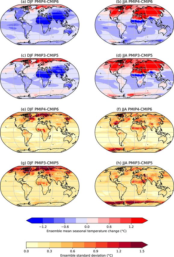
C. M. Brierley et al.: The PMIP4-CMIP6 midHolocene ensemble                                                                                                        1849

Table 1. Models contributing midHolocene simulations under CMIP6. See Table S1 for further information about the individual simulations.

                                           eq
       Model                          1T2xCO           midHolocene          piControl         Model reference                       Expt. ref. and notes
                                             2
                                          (K)              length∗            length∗
                                                            (years)            (years)
       AWI-ESM-1-1-LR                           3.6                   100          100        Sidorenko et al. (2015)               Dynamic vegetation
       CESM2                                    5.3                   700         1200        Gettelman et al. (2019)               Otto-Bliesner et al. (2020a)
       EC-Earth3-LR                             4.3                   200          200        Wyser et al. (2019)                   –
       FGOALS-f3-L                              3.0                   500          561        Wang et al. (2020)                    –
       FGOALS-g3                                2.9                   500          200        Li et al. (2020)                      –
       GISS-E2-1-G                              2.7                   100          851        Kelley et al. (2020)                  –
       HadGEM3-GC31-LL                          5.4                   100          100        Williams et al. (2018)                Williams et al. (2020)
       INM-CM4-8                                2.1                   200          531        Volodin et al. (2018)                 –
       IPSL-CM6A-LR                             4.5                   550         1200        Boucher et al. (2020)                 TSI of 1361.2 W m−2
       MIROC-ES2L                               2.7                   100          500        Hajima et al. (2020)                  Ohgaito et al. (2020)
       MPI-ESM1-2-LR                            2.8                   500         1000        Mauritsen et al. (2019)               –
       MRI-ESM2                                 3.1                   200          701        Yukimoto et al. (2019)                –
       NESM3                                    3.7                   100          100        Cao et al. (2018)                     –
       NorESM1-F                                2.3                   200          200        Guo et al. (2019)                     –
       NorESM2-LM                               2.5                   200          200        Seland et al. (2020)                  –
       UofT-CCSM-4                              3.2                   100          100        Chandan and Peltier (2017)            TSI of 1360.89 W m−2
     ∗ The lengths given are the number of simulated years used here to compute the diagnostics. These years are taken after the model has been spun up.

Table 2. Models contributing midHolocene simulations under CMIP5. See Table S1 for links to each individual simulation.

                                                                 eq
                               Model                       1T2xCO           midHolocene          piControl       Reference
                                                                 2
                                                               (K)              length∗            length∗
                                                                                 (years)            (years)
                               bcc-csm1-1                             3.1               100             500      Xin et al. (2013)
                               CCSM4                                  2.9               301            1051      Gent et al. (2011)
                               CNRM-CM5                               3.3               200             850      Voldoire et al. (2013)
                               CSIRO-MK3-6-0                          4.1               100             500      Jeffrey et al. (2013)
                               CSIRO-MK3L-1-2                         3.1               500            1000      Phipps et al. (2012)
                               EC-Earth-2-2                           4.2                40              40      Hazeleger et al. (2012)
                               FGOALS-G2                              3.7               680             700      Li et al. (2013)
                               FGOALS-S2                              4.5               100             501      Bao et al. (2013)
                               GISS-E2-R                              2.1               100             500      Schmidt et al. (2014b)
                               HadGEM2-CC                             4.5                35             240      Collins et al. (2011)
                               HadGEM2-ES                             4.6               101             336      Collins et al. (2011)
                               IPSL-CM5A-LR                           4.1               500            1000      Dufresne et al. (2013)
                               MIROC-ESM                              4.7               100             630      Sueyoshi et al. (2013)
                               MPI-ESM-P                              3.5               100            1156      Giorgetta et al. (2013)
                               MRI-CGCM3                              2.6               100             500      Yukimoto et al. (2012)
                             ∗ The lengths given are the number of simulated years used here to compute the diagnostics. These years are taken
                             after the model has been spun up.

perimental protocol on these simulations, specifically how                                2     Methods
far these changes improve known biases in the simulated
changes. We draw on an extended set of observation-derived                                2.1     Experimental set-up and models
benchmarks to evaluate these simulations. Finally we discuss
the implications of this evaluation for future climate changes,                           The protocol and experimental design for the PMIP4-CMIP6
including investigating whether changes in climate sensitiv-                              midHolocene simulations are described by Otto-Bliesner
ities between the CMIP6 and CMIP5 models has an impact                                    et al. (2017) and Earth System Documentation (2019). The
on the simulations.                                                                       midHolocene simulations are run with known orbital param-
                                                                                          eters for 6000 years BP and atmospheric trace greenhouse

https://doi.org/10.5194/cp-16-1847-2020                                                                                        Clim. Past, 16, 1847–1872, 2020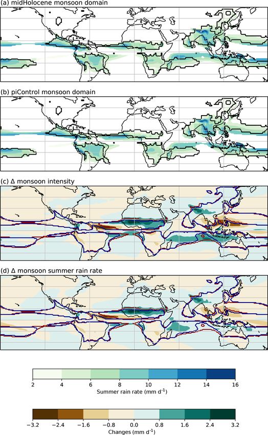
1850                                                         C. M. Brierley et al.: The PMIP4-CMIP6 midHolocene ensemble

gas concentrations (GHGs) derived from ice core records (as       tion of Wang et al. (2011) for analysis of monsoon regions: a
described by Otto-Bliesner et al., 2017). Eccentricity is in-     grid point is considered to be affected by the monsoon if the
creased by 0.001918 in the midHolocene simulations rela-          rainfall predominantly falls in the summer (May–September
tive to the piControl, obliquity is increased by 0.646◦ , and     in the Northern Hemisphere and November–March in the
perihelion (ω – 180◦ ) is changed from 100.33◦ in the pi-         Southern Hemisphere; assessed using summer rainfall form-
Control (in January) to 0.87◦ in the midHolocene (near the        ing at least 55 % of the annual total) and the average rain
boreal autumn equinox). The result of these astronomical          rate difference between summer and winter (called monsoon
changes is a difference in the seasonal and latitudinal dis-      intensity) is at least 2 mm d−1 or more. The ensemble mean
tribution of top-of-atmosphere (TOA) insolation. During bo-       global domain is determined by applying both these criteria
real summer, insolation between 40 and 50◦ N was 25 W m−2         to the ensemble mean summer rainfall and monsoon inten-
higher in the midHolocene simulations than in the piCon-          sity. We calculate annual (November–October) times series
trol (Otto-Bliesner et al., 2017). The long-lived greenhouse      of the areal extent for seven land-based monsoon systems
gases are specified at their observed concentrations. Carbon      (Christensen et al., 2013), as well as determining the aver-
dioxide is specified at 264.4 ppm (vs. 284.3 ppm during the       age precipitation rate within each system. Internal climate
pre-industrial), methane at 597 ppb (vs. 808 ppb), and N2 O       variability is characterised by the standard deviation of these
at 262 ppb (vs. 273 ppb). These changes in GHG concentra-         annual time series. The integral of these values is the total
tions lead to an effective radiative forcing of −0.3 W m−2        monsoon rainfall for each regional monsoon.
(Otto-Bliesner et al., 2017).                                        The midHolocene experiment involves redistributing the
   Sixteen models (Table 1) have performed the PMIP4-             incoming insolation spatially and through the year (Otto-
CMIP6 midHolocene simulations. A similar number of                Bliesner et al., 2017). This altered orbital configuration dur-
models have performed the equivalent PMIP3-CMIP5 mid-             ing the mid-Holocene resulted in a change in the Earth’s
Holocene simulation (Table 2). The PMIP4-CMIP6 simula-            transit speed along different parts of its orbit such that,
tions are either available from the Earth System Grid Fed-        when considered as angular fractions of the Earth’s orbit,
eration (from which they are freely downloadable) or will         the month lengths differed during the mid-Holocene (Jous-
be lodged there in the near future. We evaluate these sim-        saume and Braconnot, 1997; Bartlein and Shafer, 2019).
ulations as part of an ensemble and only sometimes iden-          Northern Hemisphere winter (December, January, February;
tify individual models. Most of the models included in the        DJF) was longer and summer (June, July, August; JJA) cor-
PMIP4-CMIP6 ensemble are state-of-the-art climate models,         respondingly shorter from an insolation perspective than in
but we also include some results from models that are ei-         the present day and the piControl simulation. However sim-
ther lower resolution or less complex (and therefore faster).     ulation output by CMIP6 models is restricted to modern cal-
Even though all models have the same orbital parameters and       endars (Juckes et al., 2020). This is not a problem for an-
trace gases in the midHolocene experiment, differences in         nual or daily diagnostics, but summarising model output us-
the specification of other boundary conditions can mean that      ing only the modern calendar prohibits straightforward ad-
the forcing is not identical in every model. For example, the     justment of the numbers of days over which the aggrega-
models may have slightly varying solar constants (see notes       tion of monthly simulation output takes place. To take ac-
in Table 1), reflecting choices made by the different groups      count of these differences in calculating monthly or seasonal
for the piControl simulations. Similarly, the orbital parame-     variables, we use the PaleoCalAdjust software (Bartlein and
ters used by some groups for the piControl are the same as        Shafer, 2019), which interpolates from non-adjusted monthly
for the historical simulation, and the trace gases are slightly   averages to pseudo-daily values and then calculates the av-
different from the PMIP4-CMIP6 recommendations. Differ-           erage values for adjusted months defined as angular frac-
ences in the pre-industrial planetary albedo, resulting from      tions of the orbit. This software has been favourably eval-
surface albedo and clouds, may also mean the effective so-        uated for monthly temperature and precipitation variations
lar forcing is different between models (Braconnot et al.,        with both PMIP4-CMIP6 and transient simulations (Bartlein
2012). Experimental set-up and spin-up procedure are doc-         and Shafer, 2019). Given the experimental protocol fixes the
umented for each midHolocene simulation individually else-        date of the vernal equinox as 21 March (Otto-Bliesner et al.,
where (following the recommendation of Otto-Bliesner et al.,      2017), the largest impact of the calendar adjustment occurs
2017).                                                            in September (a key month for Arctic sea ice coverage). The
                                                                  PaleoCalAdjust software computes adjusted monthly vari-
2.2    Analysis techniques and calendar adjustments
                                                                  ables from original monthly means, a computation which
                                                                  could impact the accuracy of variables that change abruptly
Fixed monsoon domains are often used when investigat-             throughout the year, rather than gradually, such as the sud-
ing variability and future changes in monsoon rainfall (e.g.      den increase in precipitation in monsoon regions (Pollard and
Christensen et al., 2013). However, this is not appropriate       Reusch, 2002). To explore whether potential interpolation
in the mid-Holocene when the monsoons were greatly ex-            errors from PaleoCalAdjust are justified in such situations,
tended. Following Jiang et al. (2015), we adopt the defini-       we analysed the averaged rain rate during the monsoon sea-

Clim. Past, 16, 1847–1872, 2020                                                     https://doi.org/10.5194/cp-16-1847-2020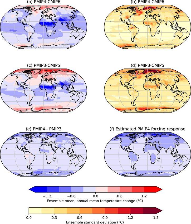
C. M. Brierley et al.: The PMIP4-CMIP6 midHolocene ensemble                                                                    1851

son over the South American monsoon domain in the IPSL-             sites in each grid cell. There is good coverage of Northern
CM6A-LR midHolocene, for which daily-resolution data are            Hemisphere terrestrial sites, although there are gaps in the
also provided on the Earth System Grid Federation. Since            coverage especially for the tropics and Southern Hemisphere
the areal extent of South American monsoon domain varies            (Bartlein et al., 2011). The Bartlein et al. (2011) dataset was
slightly when using different temporal data, we make this           extended with some speleothem and ice core temperature re-
comparison based on the grid points that always fall within         constructions and used to evaluate the PMIP3-CMIP5 simu-
the monsoon domain to provide the most robust assessment            lations (Harrison et al., 2014). In this study we use the pollen-
of the impact of the change in calendar. The average mon-           only dataset from Bartlein et al. (2011) and the multi-proxy
soon rain rate from the daily-resolution data is 7.0 mm d−1 ,       dataset (Kaufman et al., 2020b) to provide a measure of the
compared to 6.7 mm d−1 from calendar-adjusted monthly               uncertainties in reconstructed climates, although differences
data and 7.1 mm d−1 using monthly data without this ad-             in methodology and coverage preclude direct comparison be-
justment. The average monsoon rain rate in the piControl is         tween the two datasets. We incorporate an additional dataset
7.5 mm d−1 . We have therefore not applied the calendar ad-         to facilitate comparisons of the northern African monsoon
justment when analysing monsoon variables.                          between the CMIP6-PMIP4 simulations and previous gener-
   The analysis presented here mainly uses generalised eval-        ations of simulations, namely water-balance estimates of the
uation software tools derived from the Climate Variability          quantitative change in precipitation required to support the
Diagnostics Package (Phillips et al., 2014), which has been         observed mid-Holocene vegetation change at each latitude
adapted for palaeoclimate purposes (Brierley and Wainer,            compared to present (Joussaume et al., 1999).
2018). It uses the surface air temperature and precipitation
rate variables (“tas” and “pr” respectively in the ESGF con-
                                                                    3     Simulated mid-Holocene climates
trolled vocabulary; Juckes et al., 2020), as well as several
different ocean overturning mass streamfunction and sea ice         3.1    Temperature response
concentration variables.
                                                                    As expected from the insolation forcing, the PMIP4-CMIP6
2.3   Palaeoclimate reconstructions and model evaluation
                                                                    ensemble shows an increase in mean annual temperature
                                                                    (MAT) as compared to piControl conditions in the high
We provide only a preliminary quantitative evaluation of            northern and southern latitudes and over Europe (Fig. 1a).
the realism of the PMIP4-CMIP6 simulations, drawing at-             Yet there is a decrease in MAT elsewhere, which is espe-
tention to obvious similarities and mismatches between the          cially large over northern Africa and India. The ensemble
simulations and observational evidence of past climates. We         produces a global cooling of −0.3 ◦ C compared to the pi-
concentrate our evaluation on two compilations of quantita-         Control simulation (Table S2 in the Supplement). The rela-
tive reconstructions from a number of sources. We use tem-          tively small change in MAT is consistent with the fact that
perature reconstructions from the recent Temperature 12k            the midHolocene changes are largely driven by seasonal
database (Kaufman et al., 2020b). We extracted anomalies            changes in insolation. The geographic patterns of tempera-
for the mid-Holocene compared to the last millennium inter-         ture changes in the PMIP4-CMIP6 ensemble are very similar
val (from 6.0 ± 0.5 to 0.6 ± 0.5 ka) for site-level comparison      to those seen in the PMIP3-CMIP5 ensemble. However, the
with the PMIP4-CMIP6 simulations. This database has 1319            change in MAT with respect to the piControl in the PMIP4-
time series reconstructions of temperature (mean annual,            CMIP6 ensemble is generally cooler than in the PMIP3-
summer, and winter temperature) based on a variety of dif-          CMIP5 (Fig. 1). The difference in the experimental proto-
ferent ecological, geochemical, and biophysical marine (209)        col between the two sets of simulations would be expected
and terrestrial (470) sites (Kaufman et al., 2020b). Addi-          to cause a slight cooling, since the difference in GHG con-
tionally, area-averaged temperature anomalies (with respect         centrations results in an effective radiative forcing of around
to 1800–1900) over 30◦ latitudinal bands have been gener-           −0.3 W m−2 (Otto-Bliesner et al., 2017). To evaluate this, we
ated using five different methods (Kaufman et al., 2020a)           estimate the ensemble mean forced response (Fig. 1f) based
to yield a single composite value with confidence intervals.        on the climate sensitivity of each model (Table 1) and pattern
Bartlein et al. (2011) provide pollen-based reconstructions of      scaling. The estimated global mean pattern-scaled anomaly
land climate (mean annual temperature, mean temperature of          is −0.28 ◦ C, roughly similar to the difference between the
the coldest month, growing season temperature, mean annual          two model generations (Fig. 1, Table S2).
precipitation, and the ratio of actual to potential evaporation),      In line with theory, the higher insolation in Northern
although we mainly focus on mean annual temperature and             Hemisphere (NH) summer results in a pronounced summer
precipitation here. They combined the reconstructions at in-        (JJA) warming, particularly over land (Fig. 2). The increase
dividual pollen sites to produce an estimate for a 2◦ × 2◦ grid     in summer temperature over land in the NH high latitudes in
(a resolution comparable with the climate models), and re-          the ensemble mean is 1.1 ◦ C (Table S2). Increased NH sum-
construction uncertainties are estimated as a pooled estimate       mer insolation leads to a northward shift and intensification
of the standard errors of the original reconstructions for all      of the monsoons (Sect. 3.2), with an accompanying JJA cool-

https://doi.org/10.5194/cp-16-1847-2020                                                        Clim. Past, 16, 1847–1872, 2020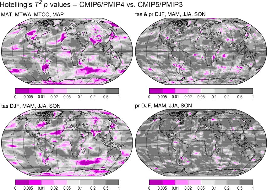
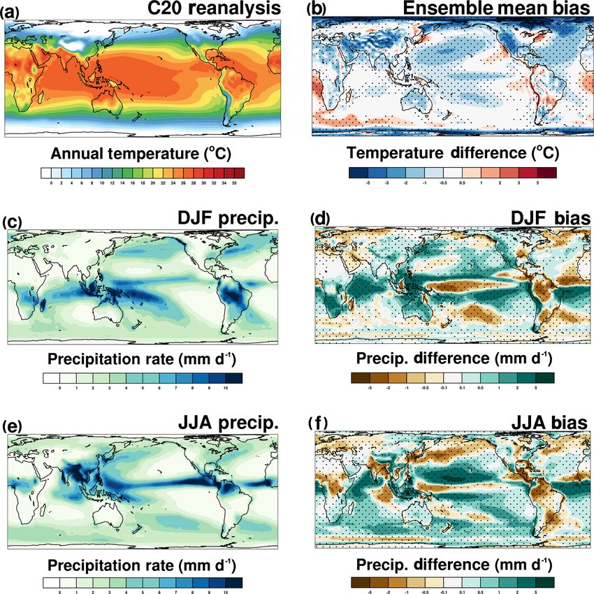
1852                                                          C. M. Brierley et al.: The PMIP4-CMIP6 midHolocene ensemble

Figure 1. Annual mean surface temperature change in the midHolocene simulations (◦ C). (a) The ensemble mean, annual mean temperature
changes in PMIP4-CMIP6 (midHolocene – piControl) and (b) the inter-model spread (defined as the across-ensemble standard deviation).
(c) The ensemble mean, annual mean temperature change in PMIP3-CMIP5 and (d) its standard deviation. (e) The difference in temperature
between the two ensembles. (f) The estimated response to the greenhouse gas concentration reductions in the experimental protocol.

ing in the monsoon-affected regions of northern Africa and           small warming of the Northern Hemisphere at the expense of
southern Asia. Reduced insolation in the NH winter (DJF)             the Southern Hemisphere in the annual, ensemble mean. The
results in cooling over the northern continents, and this cool-      PMIP4-CMIP6 ensemble is cooler than the PMIP3-CMIP5
ing extends into the northern tropical regions, although the         ensemble in both summer and winter (Fig. 2). The pattern of
Arctic is warmer than in the piControl simulation (Fig. 2).          cooling in both seasons is very similar (not shown) to the an-
Although the Southern Ocean shows warmer temperatures                nual mean ensemble difference in Fig. 1e, further supporting
in the midHolocene than the piControl simulations in austral         the lower greenhouse gas concentrations in the experimental
summer (DJF) as a result of increased obliquity, this warm-          protocol (Sect. 2.1) as the cause of the cooling.
ing does not persist into the winter to the same extent as seen         Biases in the control simulation may influence the re-
in the Arctic. The damped insolation seasonality, together           sponse to mid-Holocene forcing (Braconnot et al., 2012;
with the large effective heat capacity of the ocean, heavily         Ohgaito and Abe-Ouchi, 2009; Harrison et al., 2014; Bra-
damps seasonal variations in surface air temperature in the          connot and Kageyama, 2015) and certainly affect the pattern
Southern Ocean. The enhanced NH seasonality and the pre-             and magnitude of simulated changes. There is some diffi-
ponderance of land in the NH cause seasonal variations of            culty in diagnosing biases in the piControl, because there
the interhemispheric temperature gradient, which results in a        are few spatially explicit observations for the pre-industrial

Clim. Past, 16, 1847–1872, 2020                                                         https://doi.org/10.5194/cp-16-1847-2020
C. M. Brierley et al.: The PMIP4-CMIP6 midHolocene ensemble                                                                         1853

Figure 2. Seasonal surface temperature changes in the midHolocene simulations (◦ C). (a, b) The ensemble mean temperature changes in
PMIP4-CMIP6 (midHolocene – piControl) in DJF and JJA. (c, d) The ensemble mean temperature changes in PMIP3-CMIP5 in DJF and
JJA. The inter-model spread (defined as the across-ensemble standard deviation) in seasonal temperature changes seen across the ensembles:
(e) DJF in PMIP4-CMIP6, (f) JJA in PMIP4-CMIP6, (g) DJF in PMIP3-CMIP5, and (h) JJA in PMIP3-CMIP6.

period, especially for precipitation. We therefore evaluate            We compare these with the mean difference between the
these simulations using reanalysed climatological tempera-             pre-industrial climatology of each model (i.e. the ensemble
tures (between 1871 and 1900 CE; Compo et al., 2011) for               mean bias). The PMIP4-CMIP6 models are generally cooler
the spatial pattern (Fig. 3) and zonal averages of observed            than the observations, most noticeably in polar regions, over
temperature (Fig. 4) for the period 1850–1900 CE from the              land, and over the NH oceans (Fig. 4). The models are too
HadCRUT4 dataset (Morice et al., 2012; Ilyas et al., 2017).            warm over the eastern boundary upwelling currents, although

https://doi.org/10.5194/cp-16-1847-2020                                                             Clim. Past, 16, 1847–1872, 2020
1854                                                         C. M. Brierley et al.: The PMIP4-CMIP6 midHolocene ensemble

it remains to be seen whether this indicates improved rep-
resentation of the relevant physical processes compared to
PMIP3-CMIP5. The colder conditions over the Labrador Sea
(Fig. 3b) also indicate difficulty with resolving the regional
ocean circulation sufficiently. The polar regions are notice-
ably too cold in the ensemble mean (Fig. 3), but there is con-
siderable spread between individual models (Fig. 4). There is
no simple relationship between a model’s representation of
the pre-industrial temperature and the magnitude of its simu-
lated mid-Holocene temperature response (Fig. 4). Other fac-
tors affect the regional direct and indirect response to mid-
Holocene forcing, such as ice albedo and ocean temperature
advection into the Arctic. PMIP4-CMIP6 also includes sim-
ulations with dynamic vegetation, for example. The associ-
ated vegetation–snow-albedo feedback would tend to reduce
the simulated cooling (e.g. O’ishi and Abe-Ouchi, 2011) but
can introduce a larger cooling bias in the piControl simula-
tion (Braconnot et al., 2019). However, changes in the treat-
ment of aerosols in the PMIP4-CMIP6 ensemble could en-
hance the simulated cooling (Pausata et al., 2016; Hopcroft
and Valdes, 2019).
   Kaufman et al. (2020a) suggest that zonal, annual mean         Figure 3. Comparison of the CMIP6 ensemble to observations.
temperatures during the mid-Holocene were warmer at most          (a) The annual mean surface temperatures in the C20 reanalysis
latitudes (Fig. 4), with maximum warming in the Arctic,           (Compo et al., 2011) between 1881 and 1900. (b) The ensemble
using the reconstructions in the Temperature 12k compi-           mean difference in annual surface air temperature from the C20 re-
lation (Kaufman et al., 2020b). Individual records in the         analysis within the piControl simulations. Ability of the ensemble
Bartlein et al. (2011) compilation demonstrate the hetero-        to simulate the seasonal cycle of precipitation for the present day.
geneity within these estimates (Fig. 4). The PMIP4-CMIP6          (c, e) The precipitation climatology seen in the GPCP (Adler et al.,
                                                                  2003) observational dataset between 1971 and 2000 for DJF and
ensemble is equivocal about whether the polar regions were
                                                                  JJA respectively. (d, f) The ensemble mean difference in seasonal
warmer or cooler on the annual mean. Furthermore, the             precipitation from GPCP within the piControl simulations for DJF
PMIP4-CMIP6 models show a consistent cooling in the trop-         and JJA respectively. Stippling indicates that two-thirds of the mod-
ics. Tropical cooling was present, but less pronounced, in        els agree on the sign of the bias.
the PMIP3-CMIP5 ensemble (Fig. 4). Tropical cooling is not
consistent with the Temperature 12k area averages (Kaufman
et al., 2020a) (although the Bartlein et al., 2011, compilation
does not discount it, the majority of their reconstructions are   the extent of the simulated sea ice (Sect. 3.4). Ice–albedo
solely from Africa). Interestingly, for comparisons over Eu-      feedback would enhance inter-model temperature differences
rope and North America, both well sampled by the Bartlein         (Berger et al., 2013). The second region characterised by
et al. (2011) compilation, the models appear to show too          large inter-model differences is where there are large changes
much warming in both summer and winter (Fig. S3). Fur-            in precipitation in the tropics. This suggests that the spread
ther work is required to determine whether the discrepancies      originates in inter-model differences in simulated large-scale
between the temperature reconstructions and PMIP4-CMIP6           water advection, evaporative cooling, cloud cover, and pre-
simulations arise from systematic model error, sampling bi-       cipitation changes. There is no systematic reduction in the
ases in the data compilation (e.g. Liu et al., 2014b; Marsicek    spread of temperature responses within the PMIP4-CMIP6
et al., 2018; Rodriguez et al., 2019), or a contribution from     ensemble compared to the PMIP3-CMIP5 ensemble (Figs. 1,
both sources.                                                     2). Each of the ensembles include models of different com-
   There is substantial disagreement within the PMIP4-            plexity, and the lack of a systematic difference suggests that
CMIP6 ensemble about the magnitude of the surface temper-         complexity and model tuning has a larger impact on the re-
ature changes at the regional scale. The inter-model spread       sponses than differences in the protocol. Thus, even though
of the temperature response across the PMIP4-CMIP6 en-            there is a protocol-forced cooling of PMIP4-CMIP6 relative
semble is of the same magnitude as the ensemble mean              to PMIP3-CMIP5, these simulations can be considered sub-
for both annual (Fig. 1) and seasonal (Fig. 2) temperature        sets of a single ensemble (see Sect. 3.5; Harrison et al., 2014).
changes. There is a very large spread in the high-latitude        However, given the large inter-model range in temperature
oceans and adjacent land areas in the winter hemisphere,          changes in both subsets of this ensemble, it may be that clas-
where the spread originates from inter-model differences in       sifying the models to highlight the impact of model com-

Clim. Past, 16, 1847–1872, 2020                                                       https://doi.org/10.5194/cp-16-1847-2020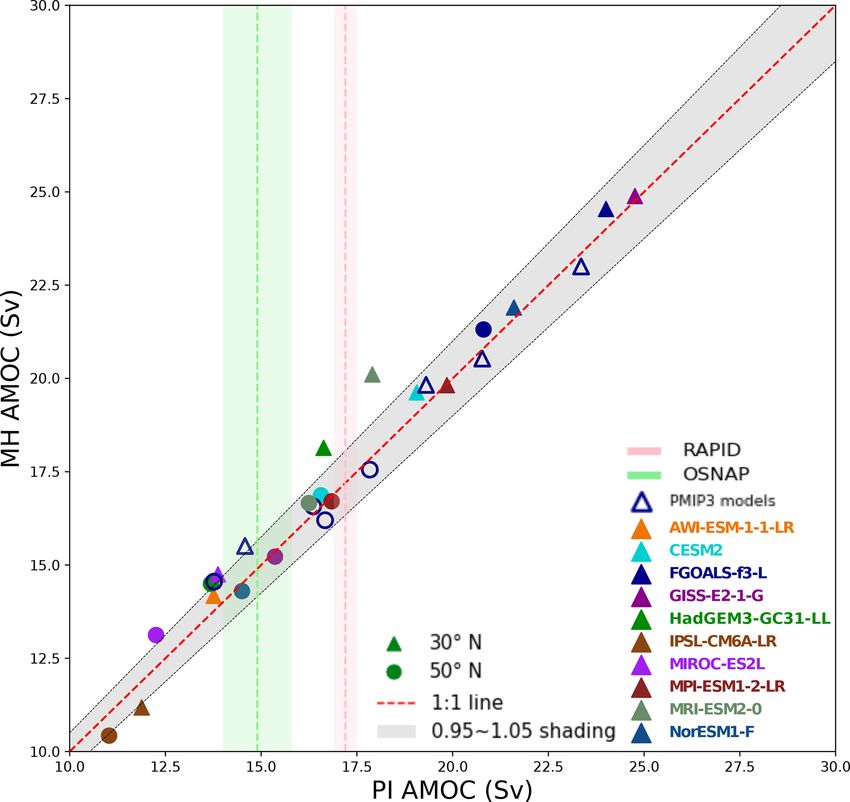
C. M. Brierley et al.: The PMIP4-CMIP6 midHolocene ensemble 1855
midHolocene simulations: this occurs because of changes in
both the summer rain rate and the monsoon intensity (Fig. 5).
The weakening of the annual range of precipitation over the
ocean and the strengthening over the continents indicate the
changes reflect a redistribution of moisture (see e.g. Bracon-
not, 2004).
The most pronounced and robust changes in the mon-
soon occur over northern Africa and the Indian subcontinent
(Fig. 6). The areal extent of the northern African monsoon
is 20 %–50 % larger than in the piControl simulations, but
the average rain rate only increases by 10 % (Fig. 7). The in-
tensification of precipitation on the southern flank of the Hi-
malayas (Table S2) in the midHolocene simulations is offset
by a reduction in the Philippines and Southeast Asia (Fig. 6),
so the area-averaged reduction in rain rate is reduced over the
South Asian monsoon domain (Fig. 7). There is an extension
and intensification of the East Asian monsoon that is con-
sistent across the PMIP4-CMIP6 ensemble, but the change
is < 10 % (Fig. 7). Ensemble mean changes in the North
American Monsoon System, and the Southern Hemisphere
monsoons are also small (Fig. 6) and less consistent across
the ensemble although most of the models show a weaken-
ing and contraction of the South American Monsoon Sys-
tem and southern African monsoon (Fig. 7). Changes in in-
ternal climate variability within the monsoon systems (char-
acterised by standard deviations of the annual time series of
both the areal extent and area-averaged rain rate; Fig. 7) are
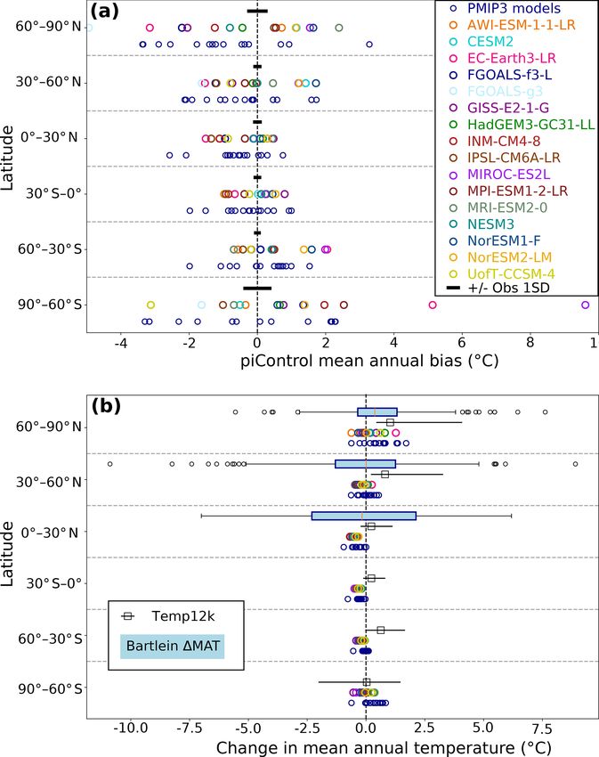
Figure 4. Zonal averaged temperatures within the PMIP4-CMIP6
ensemble. (a) Comparison of the piControl zonal mean temperature not consistent across the PMIP4-CMIP6 ensemble. Further-
profile of individual climate models to the 1850–1900 observations. more, those models that have the largest change in variability
The area-averaged, annual mean surface air temperature for 30◦ lat- in one region are not necessarily the models that have large
itude bands in the CMIP6 models (identified), CMIP5 models (blue changes in other regions, which suggests that this variability
circles), and a spatially complete compilation of instrumental ob- is linked with regional feedbacks, rather than being an inher-
servations over 1850–1900 (black, Ilyas et al., 2017; Morice et al., ent characteristic of a model.
2012). (b) The simulated annual mean temperature change averaged The broadscale changes in the PMIP4-CMIP6 simulations,
over 30◦ zonal bands for each of the individual CMIP6 models. with weaker southern and stronger/wider Northern Hemi-
The equivalent changes estimated from the Temperature 12k com- sphere monsoons, were present in the PMIP3-CMIP5 simu-
pilation (Kaufman et al., 2020b) via a multi-method approach are
lations (Fig. 6; testing the significance of the differences be-
shown along with their 80 % confidence interval. The distribution
tween the ensembles is discussed in Sect. 3.5). The response
of Bartlein et al. (2011) reconstructed temperatures within each lat-
itude bands are shown in the NH, because the tropical and Southern is robust across model results, indicating that all models pro-
Hemisphere latitudes are only represented by sites in Africa. The duce the same large-scale redistribution of moisture by the
data points for all models, as well as the equivalents over land or atmospheric circulation in response to the interhemispheric
ocean, are provided in the Supplement. and land–sea gradients induced by the insolation and trace
gas forcing. At a regional scale, however, there are differ-
ences between the two ensembles. The PMIP4-CMIP6 mid-
plexity or of model biases on the climate response would be Holocene ensemble shows wetter conditions over the Indian
useful. This would also allow selection of subsets of the mod- Ocean, a larger northward shift of the Intertropical Con-
els for specific analyses, following a fit-for-purpose approach vergence Zone (ITCZ) in the Atlantic, and a widening of
(Schmidt et al., 2014a). the Pacific rain belt compared to the PMIP3-CMIP5 mod-
els (Fig. 6). The expansion of the summer (JJA) monsoon
3.2 Monsoonal response
in northern Africa is also greater in the PMIP4-CMIP6 than
the PMIP3-CMIP5 ensemble (Table S2), and the location of
The enhancement of the global monsoon is the most impor- the northern boundary is more consistent between models.
tant consequence of the mid-Holocene changes in seasonal This is associated with a better representation of the north-
insolation for the hydrological cycle (Jiang et al., 2015). The ern edge of the rain belt for the piControl simulation in
global monsoon domain is expanded in the PMIP4-CMIP6 the PMIP4-CMIP6 ensemble compared with previous gen-
https://doi.org/10.5194/cp-16-1847-2020 Clim. Past, 16, 1847–1872, 2020
1856                                                           C. M. Brierley et al.: The PMIP4-CMIP6 midHolocene ensemble

Figure 5. PMIP4-CMIP6 ensemble mean global monsoon domain (mm d−1 ). The monsoon domain for each simulation is identified by
applying the definitions of Wang et al. (2011) and in Sect. 2.2 to the PMIP4-CMIP6 ensemble mean of both (a) the midHolocene and (b) the
piControl simulations. The black contour in panels (a) and (b) shows the boundary of the domain derived from present-day observations
(Adler et al., 2003). The simulated changes in the monsoon domain are determined by changes in both (c) the monsoon intensity – average
rain rate difference between summer and winter – and (d) the summer rain rate. In panels (c) and (d) the red and blue contours show the
boundary of midHolocene and piControl global monsoon domains respectively.

erations (Fig. S1). However, there is little relationship be-         local temperature variations (D’Agostino et al., 2019, 2020).
tween the piControl precipitation biases and the simulated            The modulation of this dynamical response by the land sur-
midHolocene changes in precipitation (Fig. S1). The varia-            face and vegetation components of the PMIP4-CMIP6 mod-
tions in the midHolocene rainfall signal appear to be more            els should be investigated.
related to monsoon dynamics rather than orbitally induced

Clim. Past, 16, 1847–1872, 2020                                                           https://doi.org/10.5194/cp-16-1847-2020
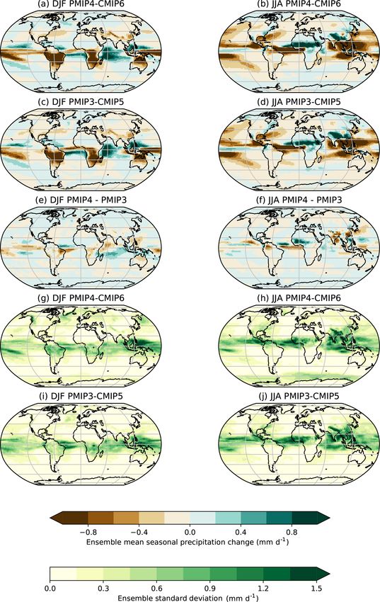
C. M. Brierley et al.: The PMIP4-CMIP6 midHolocene ensemble                                                                      1857

Figure 6. The midHolocene seasonal changes in precipitation (mm d−1 ). (a, b) The ensemble mean precipitation changes in PMIP4-CMIP6
(midHolocene – piControl) in DJF and JJA. (c, d) The ensemble mean precipitation changes in PMIP3-CMIP5 in DJF and JJA. (e, f) The
differences in DJF and JJA precipitation between the PMIP4-CMIP6 and PMIP3-CMIP5 ensembles. The inter-model spread (defined as
the across-ensemble standard deviation) in seasonal precipitation changes seen across the ensembles: (g) DJF in PMIP4-CMIP6, (h) JJA in
PMIP4-CMIP6, (i) DJF in PMIP3-CMIP5, and (j) JJA in PMIP3-CMIP6.

https://doi.org/10.5194/cp-16-1847-2020                                                           Clim. Past, 16, 1847–1872, 2020
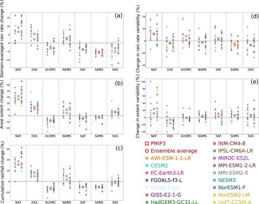
1858                                                              C. M. Brierley et al.: The PMIP4-CMIP6 midHolocene ensemble

Figure 7. Relative changes in individual midHolocene monsoons. Five different monsoon diagnostics (see Sect. 2.2) are computed for
each of seven different regional domains (Christensen et al., 2013). (a) The change in area-averaged precipitation rate during the monsoon
season (May–September) for each individual monsoon system. (b) The change in the areal extent of the regional monsoon domains. (c) The
percentage change in the total amount of water precipitated in each monsoon season (computed as the precipitation rate multiplied by
the areal extent). (d) Change in the standard deviation of interannual variability in the area-averaged precipitation rate. (e) The change in
standard deviation of the year-to-year variations in the areal extent of the regional monsoon domain. The abbreviations used to identify each
regional domain are North American Monsoon System (NAMS), northern Africa (NAF), southern Asia (SAS), and East Asia summer (EAS)
in the Northern Hemisphere and South American Monsoon System (SAMS), southern Africa (SAF), and Australian–Maritime Continent
(AUSMC) in the Southern Hemisphere.

   Although the PMIP4-CMIP6 models show the expected                     ulations (Fig. 5). Furthermore, evaluation of the piControl
expansion of the monsoons, this expansion is weaker than                 simulations using climatological precipitation data for the
indicated by palaeoclimate reconstructions (Figs. 8 and S3).             period between 1970 and the present day (Adler et al., 2003)
This was a feature of the PMIP3-CMIP5 simulations (Bra-                  shows the models fail to capture the magnitude of rainfall
connot et al., 2012; Perez-Sanz et al., 2014) and previous               in the ITCZ and the southern portion of the South Pacific
generations of climate models (Joussaume et al., 1999; Bra-              Convergence Zone (SPCZ). The SPCZ is too zonal because
connot et al., 2007). It has been suggested that this per-               of the poor representation of the sea surface temperature
sistent mismatch between simulations and reconstructions                 (SST) gradient between the Equator and 10°S in the west
arises from biases in the piControl (Harrison et al., 2015).             Pacific (Fig. 3; Brown et al., 2013; Saint-Lu et al., 2015).
Indeed, the ensemble mean global monsoon domain in the                   The PMIP4-CMIP6 models exhibit a dry bias over tropi-
PMIP4-CMIP6 ensemble is more equatorward in the piCon-                   cal and high-northern-latitude land areas, although the mid-
trol compared to the observations, particularly over the ocean           latitude storm tracks are captured with varying levels of fi-
(Fig. 5). In northern Africa, the expansion of the monsoon               delity (Fig. 3).
domain in the midHolocene simulations merely removes the                    There are large differences in the simulated change in mid-
underestimation of its poleward extent in the piControl sim-             Holocene precipitation between different models, as shown

Clim. Past, 16, 1847–1872, 2020                                                              https://doi.org/10.5194/cp-16-1847-2020
C. M. Brierley et al.: The PMIP4-CMIP6 midHolocene ensemble                                                                        1859

Figure 8. Comparison between simulated annual precipitation changes and pollen-based reconstructions (from Bartlein et al., 2011). Seven
regions where multiple quantitative reconstructions exist are chosen. Six of them are defined following Christensen et al. (2013) and are
northern Europe (NEU), central Europe (CEU), the Mediterranean (MED), the Sahara/Sahel (SAH), East Asia (EAS) and eastern North
America (ENA). Mid-continental Eurasia (B17) is specified by Bartlein et al. (2017) as 40–60◦ N, 30–120◦ E. The distribution of recon-
structions within the region are shown by boxes and whiskers. The area-averaged change in mean annual precipitation simulated by CMIP6
(individually identifiable) and CMIP5 (blue) within each region is shown for comparison (following Flato et al., 2013).

by the standard deviation around the ensemble mean, in both            continental temperatures is inconsistent with palaeoenviron-
the PMIP4-CMIP6 and PMIP3-CMIP5 ensembles (Figs. 6                     mental evidence (and climate reconstructions), which show
and 8). Unsurprisingly, the largest differences between mod-           that this region was characterised by wetter and cooler con-
els occur where the simulated change in precipitation is also          ditions than today in the mid-Holocene (Fig. 8; Bartlein et al.,
largest (Fig. 6).                                                      2017, Table S2). This indicates that model improvements
                                                                       have not resolved the persistent mismatch between simulated
3.3   Extratropical hydrological responses                             and observed mid-Holocene climate. Bartlein et al. (2017)
                                                                       pinpointed biases in the simulation of the extratropical at-
Hydrological changes in the extratropics are comparatively             mospheric circulation as the underlying cause of this mis-
muted in the PMIP4-CMIP6 ensemble and closely resemble                 match. The higher resolution of most PMIP4-CMIP6 models
features seen in the PMIP3-CMIP5 ensemble. There is a re-              does not seem to improve the representation of these aspects
duction in rainfall at the equatorward edge of the mid-latitude        of the circulation. Imperfect simulation of the extratropical
storm tracks, most noticeable over the ocean (Fig. 6). The             circulation could also explain the failure to capture precipita-
NH extratropics are generally drier in the midHolocene sim-            tion changes over Europe accurately (Mauri et al., 2014). The
ulations than in the piControl. There is a large inter-model           PMIP4-CMIP6 ensemble shows little change in mean annual
spread in the summer rainfall changes over eastern North               precipitation over Europe (Fig. 6). Reconstructions of mid-
America and central Europe (Fig. 8). The spread in summer              Holocene precipitation suggest modest increases in northern
rainfall in both regions is clearly related to the large inter-        Europe, increases in central Europe, and much wetter condi-
model spread in summer temperature (cf. Figs. 2 and 6). Re-            tions in the Mediterranean – something which is not captured
constructions from eastern North America suggest slightly              by the PMIP4-CMIP6 ensemble (Figs. 8, S3).
drier conditions while reconstructions for central Europe
show somewhat wetter conditions, but in neither case are
                                                                       3.4   Ocean and cryospheric changes
these incompatible with the simulations.
   There are regions, however, where there is a substantial            The Atlantic Meridional Overturning Circulation (AMOC)
mismatch between the PMIP4-CMIP6 simulations and the                   is an important factor affecting the Northern Hemisphere
pollen-based reconstructions. There is a simulated reduction           climate system and is a major source of decadal and mul-
in summer rainfall in mid-continental Eurasia (Fig. 6). This           tidecadal climate variability (e.g. Rahmstorf, 2002; Lynch-
reduction is somewhat larger in the PMIP4-CMIP6 ensem-                 Stieglitz, 2017; Jackson et al., 2015). Recent studies have
ble than in the PMIP3-CMIP5 ensemble, although this dif-               reported a decline of up to ∼ 15 % in AMOC strength
ference is likely not significant (Fig. 8). However, this re-          from the pre-industrial period to the present day (Rahm-
duction in precipitation and the consequent increase in mid-           storf et al., 2015; Dima and Lohmann, 2010; Caesar et al.,

https://doi.org/10.5194/cp-16-1847-2020                                                            Clim. Past, 16, 1847–1872, 2020
1860 C. M. Brierley et al.: The PMIP4-CMIP6 midHolocene ensemble
2018; Thornalley et al., 2018), at least partly in response
to anthropogenic forcing. Reproducing the AMOC of the
mid-Holocene is important for understanding the climate
responses to external forcing at millennial timescales. The
members of both the PMIP4-CMIP6 and PMIP3-CMIP5 en-
semble have different AMOC strengths in their piControl
simulations (Fig. 9), although all models correctly predict
that it is stronger at 30◦ N than at 50◦ N. The PMIP4-CMIP6
models project a consistent reduction in AMOC under fu-
ture scenarios (Weijer et al., 2020). There is a strong correla-
tion (r = 0.99 at 30◦ N) between the simulated strength of the
AMOC in the midHolocene and the piControl. Furthermore,
there is little change in the overall strength of the AMOC be-
tween the midHolocene and piControl experiments (Fig. 9)
in either the PMIP4-CMIP6 or the PMIP3-CMIP5 simula-
tions and no consistency in whether this comparatively small
(and probably non-significant) change is positive or negative.
Using a single metric to categorise changes in the AMOC
is awkward – that two measures, both with their own un-
certainties, indicate the same result increases our confidence
that the overall changes were small. Shi and Lohmann (2016) Figure 9. Atlantic Meridional Overturning Circulation (AMOC)
detect large differences in simulated AMOC anomalies be- in the simulations. The strength of the AMOC is defined as the
tween models with coarse and higher resolutions. They sug- maximum of the mean meridional mass overturning streamfunction
gest ocean and atmospheric processes affecting ocean salin- below 500 m at 30 and 50◦ N in the Atlantic. The strength in the
ity close to the sites of deep convection mean that higher- piControl simulation provides the horizontal axis, whilst the ver-
tical location is given by the strength in the midHolocene simula-
resolution models tend to produce stronger midHolocene
tion. Data points lying on the 1 : 1 line demonstrate no change be-
AMOC and lower-resolution simulations a weaker AMOC tween the two simulations. Observational estimates of the present-
than the piControl. The comparatively small changes in the day AMOC strength are shown from both the RAPID-MOCHA ar-
AMOC strength between the PMIP4-CMIP6 piControl and ray (at 26◦ N, Smeed et al., 2019) and the OSNAP section (between
midHolocene simulations are consistent with these earlier re- 53 and 60◦ N, Lozier et al., 2019).
sults, where the simulated changes are generally of less than
2 Sv (Fig. 9).
It is difficult to reconstruct past changes in the AMOC, the amount of sea ice reduction was related to the magnitude
especially its depth-integrated strength. Previous analy- of warming in the region (Berger et al., 2013; Park et al.,
ses have focussed on examining individual components 2018). These findings hold for the PMIP4 models (Fig. 10).
of the AMOC, for example by using sediment grain size The PMIP4-CMIP6 models have slightly more realistic sen-
(Hoogakker et al., 2011; Thornalley et al., 2013; Moffa- sitivities of Arctic sea ice to warming and greenhouse gas
Sanchez et al., 2015). The overall strength of the AMOC may forcing than PMIP3-CMIP5 models, but their simulated sea
be constrained by using sedimentary Pa/Th (e.g. McManus ice extents cover the same large spread easily encompassing
et al., 2004), although geochemical observations show that the observations (SIMIP Community, 2020). There is little
several additional factors influence Pa and Th distribution Arctic-wide relationship between the pre-industrial sea ice
(Hayes et al 2013). The available Pa/Th records indicate no extent and its reduction at the mid-Holocene (Fig. 10). Lo-
significant change in the AMOC between the mid-Holocene cal relationships may hold for key regions, such as the North
and the pre-industrial period (McManus et al., 2004; Ng Atlantic, where connections between pre-industrial sea ice
et al., 2018; Lippold et al., 2019). Reconstruction of changes coverage and mid-Holocene AMOC and summer sea ice re-
in the upper limb of the AMOC, based on geostrophic esti- ductions have been observed (Găinuşă-Bogdan et al., 2020).
mates of the Florida Straits surface flow, also indicates lit- The changes in Arctic sea ice extent simulated for the mid-
tle change over the past 8000 years (Lynch-Stieglitz et al., Holocene are generally amplified by the stronger insolation
2009). Thus, overall, the palaeo-reconstructions are consis- forcing imposed in the lig127k experiment (Otto-Bliesner
tent with the simulated results (Fig. 9). et al., 2020b). Prior statistical analysis (Berger et al., 2013)
The altered distribution of incoming solar radiation at the supported by recent process-based understanding (SIMIP
mid-Holocene would be expected to alter the seasonal cycle Community, 2020) suggests that further analysis of mid-
of sea ice concentration. Analysis of simulations from pre- Holocene sea ice changes would be informative for future
vious generations of PMIP found a consistent reduction in Arctic projections (Yoshimori and Suzuki, 2019).
Arctic summer sea ice extent at the mid-Holocene and that
Clim. Past, 16, 1847–1872, 2020 https://doi.org/10.5194/cp-16-1847-2020C. M. Brierley et al.: The PMIP4-CMIP6 midHolocene ensemble 1861
Figure 10. Changes in Arctic sea ice minimum extent. The change in the areal extent of the minimum sea ice cover (i.e. grid boxes with
greater than 15 % concentration) at the mid-Holocene compared to (a) the minimum sea ice extent in the piControl simulations and (b) the
Arctic annual mean temperature change. Observational estimates of the pre-industrial extent (Walsh et al., 2016) and mid-Holocene Arctic
warming (Fig. 4; Kaufman et al., 2020a) are also shown.
3.5 Evaluation of mid-Holocene climate features AMOC, suggest that the PMIP4-CMIP6 simulations should
be regarded as from the same population as the PMIP3-
Comparisons of the PMIP4-CMIP6 simulations with either CMIP5 simulations. We formally test this by calculating
palaeoenvironmental observations or palaeoclimate recon- Hotelling’s T 2 statistic (Wilks, 2011), a multivariate gener-
structions have highlighted a number of regions where there alisation of the ordinary t statistic that is often used to exam-
are mismatches either in magnitude or sign of the simulated ine differences in climate model simulations (Chervin and
response. The combination of the mismatches in, for exam- Schenider, 1976), at each grid point of a common 1◦ grid for
ple, simulated mean annual temperature or temperature sea- different combinations of climate variables. The patterns of
sonality results in an extremely poor overall assessment of significant (i.e. p < 0.05) tests (where one would reject the
the performance of each model (Fig. S2). This global as- null hypothesis that the PMIP4-CMIP6 and PMIP3-CMIP6
sessment also provides little basis for discriminating between ensemble means are equal) are random (Fig. 11) and show
models, a necessary step in using the quality of specific mid- little relation to the largest climate anomalies (Figs. 1 and 6).
Holocene simulations operationally to enhance future pro- The total number of significant grid cells does not exceed the
jections for climate services (Schmidt et al., 2014a). At a re- false discovery rate (Wilks, 2006). Consequently there is lit-
gional scale (Figs. 4, 8, S3) it is clearly possible to identify tle support for the idea that the PMIP4-CMIP6 generation
models that are unable to reproduce the observations satis- of simulations differ from the PMIP3-CMIP5 simulations,
factorily. Thus, there would be utility in making quantitative which were themselves not significantly different from the
assessment of model performance at a regional scale. Com- PMIP2-CMIP3 simulations (Harrison et al., 2015). This sug-
bining regional benchmarking of model performance with gests that all of these simulations could be considered as a
process diagnosis – to ensure that a model is correct because single ensemble for process-based analysis (e.g. D’Agostino
it captures the right processes – would therefore provide a et al., 2019, 2020) or for the investigation of emergent con-
firmer basis for using the midHolocene simulations to en- straints (Yoshimori and Suzuki, 2019). Combining models
hance our confidence in future projections. from multiple ensembles could considerably enhance the sta-
Analyses of key features of the midHolocene simulations, tistical power of such analyses.
such as the monsoon amplification or the strength of the
https://doi.org/10.5194/cp-16-1847-2020 Clim. Past, 16, 1847–1872, 2020You can also read