Remote Sensing Based Pre-Season Yellow Rust Early Warning in Oromia, Ethiopia

Master Thesis in Geographical Information Science nr 126

 Remote Sensing Based Pre-Season
 Yellow Rust Early Warning in
 Oromia, Ethiopia

Chinatsu Endo

2021
Department of
Physical Geography and Ecosystem Science
Centre for Geographical Information Systems
Lund University
Sölvegatan 12
S-223 62 Lund
Sweden

Chinatsu Endo (2021). Remote Sensing Based Pre-Season Yellow Rust Early
Warning in Oromia, Ethiopia

Master degree thesis, 30/ credits in Master in Geographical Information Science
Department of Physical Geography and Ecosystem Science, Lund University

 ii

Remote Sensing Based Pre-Season Yellow Rust
 Early Warning in Oromia, Ethiopia

 Chinatsu Endo
 Master thesis, 30 credits, in Geographical Information Sciences

 Supervisors:

 Associate Professor Dr. Kees de Bie,
 ITC, The University of Twente, The Netherlands

 Associate Professor Dr. David E. Tenenbaum,
 Lund University, Sweden

 iii

iv

Abstract
Yellow rust (Puccinia striiformis f. sp. Tritici) is a crop disease of wheat that regularly
causes yield loss in Ethiopia. The disease has significant consequences for the country’s
crop production, food security, health, and socioeconomic well-being. Anticipating
yellow rust epidemics can help better manage them and mitigate their adverse impacts.
This study explores the potential of remote sensing-based early prediction of yellow rust
in the Oromia region in Ethiopia. The research focuses on modeling the incidence of
yellow rust among young wheat in the region by looking at unique environmental
conditions that enable off-season survival of the rust pathogen.

Tiller and boot-level yellow rust incidence data from 2016-2018 in Oromia was analyzed
together with the environmental variables generated through AgERA5 (temperature),
CHIRPS (precipitation), ProbaV-NDVI, and SRTM-DEM (terrain characteristics).
Univariate Area Under ROC Curve analysis and Classification Tree analysis were used
to understand the influential environmental variables and filter those with high relevance
to the early-stage rust infection. Subsequently, General Additive Model and Boosted
Regression Tree were applied to fit and test the early warning models and their prediction
capacity. The models were built for three data sets: data with all available observations;
tiller-level observations; and data that share the same climate zone.

As a result, the climate zone-based GAM model performed at a 78% accuracy level with
Kappa 0.44 (moderate). The tiller-only GAM model performed at a 72% accuracy level
with Kappa 0.44 (moderate). The all-observation BRT model had a 71% accuracy level
with Kappa 0.34 (fair agreement). Rain characteristics served as particularly strong
predictors in these models. Especially, excessive rain had a strong relationship with a
lower probability of yellow rust cases among young wheat. The models also suggest that
terrain characteristics serve as the static environmental conditions that expose certain
locations to the disease. The study demonstrated the potential of yellow rust early warning
solely based on remote sensing. The models could be further tested with a larger volume
of data set to confirm the strength. Consideration of the probability of varying rust
severity (low, moderate, high) and types of wheat cultivars would further add value to the

 v

models. Lastly, additional field and laboratory-based knowledge on the off-season rust
survival would be a vital step towards a more accurate configuration of early warning
models.

 vi

Acknowledgments

This study was realized with the support from the International Maize and Wheat
Improvement Center (CIMMYT) in Ethiopia through the timely provision of rust survey
data. Special appreciation goes to Dr. David Hodson, Mr. Yoseph Alemayehu, and Dr.
Gerald Blasch at CIMMYT for their time and guidance during the data collection phase.

I want to thank my supervisors, Associate Professor Dr. Kees de Bie at Twente University
and Associate Professor Dr. David E. Tenenbaum at Lund University, for guiding the
design and execution of my final project. Special thanks to Ir. Louise Van Leeuwen at
Twente University for encouraging me to pursue the on-campus study in early 2020.
Despite the limitation and challenges during the COVID-19 pandemic, this visit enriched
my learning experience as an iGEON distance student. Finally, completion of the degree
would have been impossible without the understanding of my husband. Thank you, Dan,
for your unconditional support for my journey of learning.

 vii

viii

Table of Contents

Abstract v
Acknowledgments vii
List of Abbreviations xi
List of Figures xii
List of Tables xiv
1. Introduction 1
 Objectives and Research Questions 2
2. Background 5
 2.1 Yellow Rust 5
 2.2 Oversummering and Overwintering of Yellow Rust 8
 2.3 Yellow Rust Prediction Models 9
 2.4 Knowledge Gap 11
3. Method 13
 3.1 Study Area 13
 3.2 Methodological Flowchart 14
 3.3 Data 15
 3.4 Data Processing 18
 3.5 Analysis 22
 3.5.1 Variable Exploration (RQ1.a) 22
 3.5.2 Finding the most critical variables (RQ1.b) 23
 3.5.3 Assessing Model Predictive Capacity (RQ2) 26
 3.5.4 Model Extrapolation over Oromia Region 28
4. Results 29
 4.1 Understanding Oromia’s Wheat Growing Environment 29
 4.2 Association between rust incidence and pre-season environmental condition 33
 Summary of variable exploration 42
 4.3 Most Influential Environmental Parameters 43
 4.4 Prediction and Accuracy 54
 4.5 Model Extrapolation 55
5. Discussion 57
 Rainfall as a critical parameter 57
 How early is early enough? 58
 Role of static environmental characteristics 58
 Strength of Models 58

 ix

Opportunities for RS-based ‘earlier’ warning of yellow rust 59
6. Conclusion 63
REFERENCE 65
APPENDICES 70
Series from Lund University 78

 x

List of Abbreviations

 AUC Area Under the ROC Curve
 BRT Boosted Regression Tree
 CHIRPS Climate Hazards Group InfraRed Precipitation with Station data
 CIMMYT International Maize and Wheat Improvement Center
 CT Classification Tree
 DN Digital Number
 ECMWF European Center for Medium-range Weather Forecast
 AgERA5 Agriculture ERA5
 European Center for Medium-range Weather Forecast Reanalysis
 ERA5
 5th Generation
 FAO Food and Agriculture Organization
 FEWS NET Famine Early Warning Systems Network
 FN False Negative
 FP False Positive
 GAM General Additive Model
 GEE Google Earth Engine
 GIS Geographic Information System
 GLM Generalized Linear Model
 NASA National Aeronautics and Space Administration
 NDVI Normalized Difference Vegetation Index
 NOAA National Oceanic and Atmospheric Administration
 Pst. Puccinia Striiformis f. sp. Tritici
 ROC Receiver Operating Characteristic
 RQ Research Question
 RS Remote Sensing/Remotely Sensed
 SRTM Shuttle Radar Topography Mission
 TN True Negative
 TP True Positive
 USAID United States Agency for International Development
 USDA United States Department of Agriculture
 USGS United States Geological Survey
 VIF Variance Inflation Factor
 WGS83 World Geodetic System 1984

 xi

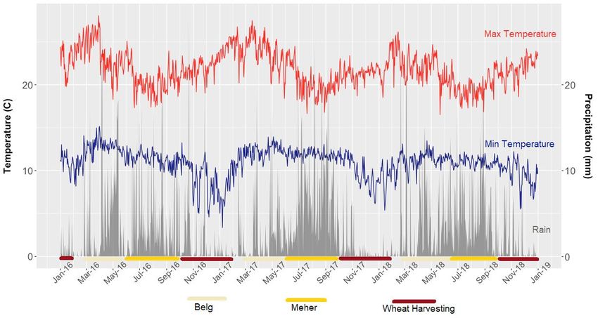
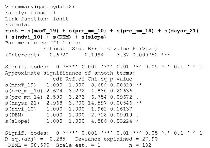
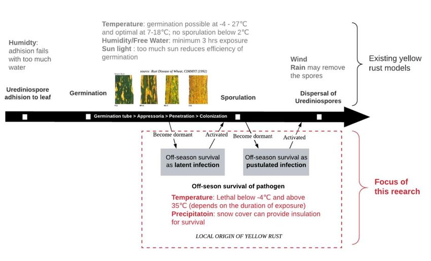
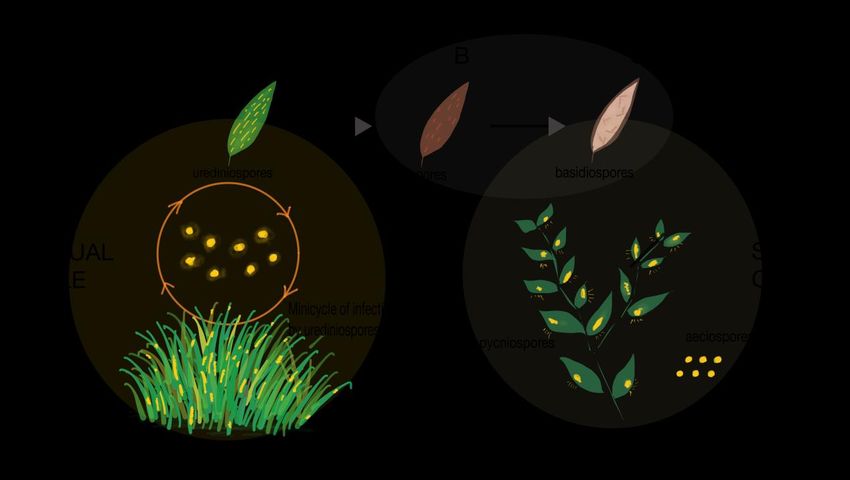
List of Figures

FIGURE 1: ADULT PLANT HOST RESPONSE TO YELLOW RUST ........................................................................................ 5
FIGURE 2: SYMPTOMS AND SPORE (UREDINIOSPORE) MORPHOLOGY OF YELLOW RUST DISEASE ......................................... 5
FIGURE 3: LIFECYCLE OF PUCCINIA STRIIFORMIS F. SP. TRITICI (PST) ON PRIMARY HOST AND ALTERNATE HOST ..................... 6
FIGURE 4: PROPAGATION OF INFECTION ON LEAVE BY A UREDINIOSPORE ...................................................................... 7
FIGURE 5: GROWTH CYCLE OF WHEAT INFLUENCED BY THE RUST INFECTION ON VOLUNTEER WHEAT .................................. 9
FIGURE 6: FOCUS OF THIS STUDY IN RELATION WITH THE EXISTING YELLOW RUST MODELS AND STAGES OF PTS INFECTION.... 12
FIGURE 7: MAP OF STUDY AREA - OROMIA REGION, ETHIOPIA ................................................................................. 13
FIGURE 8: METHODOLOGICAL FLOWCHART .......................................................................................................... 14
FIGURE 9: NDVI PROFILE BY GROUP (CLIMATE ZONE) ............................................................................................. 20
FIGURE 10: MAP OF MAJOR CLIMATE ZONES IN OROMIA REGION ............................................................................. 21
FIGURE 11: CONFUSION MATRIX ........................................................................................................................ 27
FIGURE 12: TEMPERATURE (MAX, MIN) AND PRECIPITATION AT THE RUST OBSERVATION POINTS IN OROMIA 2016–2018 . 29
FIGURE 13: DISTRIBUTION OF YELLOW RUST OBSERVATION POINTS IN OROMIA REGION ................................................ 30
FIGURE 14: PROPORTION OF DIFFERENT WHEAT VARIETIES GROWN IN OROMIA REGION ............................................... 31
FIGURE 15: AUC VALUES (ALL OBSERVATIONS) ..................................................................................................... 33
FIGURE 16: CLASSIFICATION TREES (ALL OBSERVATIONS) ......................................................................................... 36
FIGURE 17: AUC VALUES (TILLER-ONLY) .............................................................................................................. 37
FIGURE 18: CLASSIFICATION TREES (TILLER-ONLY).................................................................................................. 39
FIGURE 19: AUC VALUES (CLIMATE ZONE B) ........................................................................................................ 40
FIGURE 20: CLASSIFICATION TREES (CLIMATE ZONE B)............................................................................................ 42
FIGURE 21: GAM SUMMARY (ALL OBSERVATION).................................................................................................. 43
FIGURE 22: GAM PARTIAL EFFECT PLOT (ALL OBSERVATIONS) ................................................................................. 44
FIGURE 23: BOX CHART OF NDVI TREND (ALL OBSERVATIONS)................................................................................. 46
FIGURE 24: BRT OPTIMAL NUMBER OF TREES (ALL OBSERVATIONS)........................................................................... 47
FIGURE 25: BRT VARIABLE INTERACTION BETWEEN ALTITUDE AND SLOPE (ALL OBSERVATION) ........................................ 48
FIGURE 26: BRT VARIABLE INTERACTION BETWEEN ALTITUDE AND DAYSR_21 (ALL OBSERVATION) ................................. 48
FIGURE 27: GAM SUMMARY (TILLER-ONLY) ......................................................................................................... 49
FIGURE 28: GAM PARTIAL EFFECT PLOT (TILLER-ONLY) .......................................................................................... 50
FIGURE 29: BRT OPTIMAL NUMBER OF TREES (TILLER-ONLY).................................................................................... 51
FIGURE 30: BRT VARIABLE INTERACTION BETWEEN MAXT_12 AND DAYSR_21 (TILLER-ONLY) ....................................... 51
FIGURE 31: BRT VARIABLE INTERACTION BETWEEN DAYSR_21 AND ASPECT (TILLER-ONLY) ............................................ 52
FIGURE 32: GAM SUMMARY (ZONE.B) ................................................................................................................ 53
FIGURE 33: GAM PARTIAL EFFECT PLOT (ZONE.B) ................................................................................................ 53

 xii

FIGURE 34: YELLOW RUST PROBABILITY MAPS WITH THE TILLER-ONLY GAM MODEL..................................................... 55
FIGURE 35: YELLOW RUST PROBABILITY MAP FOR CLIMATE ZONE BASED ON THE ZONE.B GAM MODEL ........................... 56

 xiii

List of Tables

TABLE 1: YELLOW RUST INCIDENCE DATA USED IN THE STUDY ................................................................................... 15
TABLE 2: LIST OF RS-BASED PRODUCTS FOR DYNAMIC ENVIRONMENTAL CONDITIONS ................................................... 16
TABLE 3: LIST OF RS-BASED PRODUCTS FOR STATIC ENVIRONMENTAL CONDITIONS ....................................................... 16
TABLE 4: ENVIRONMENTAL VARIABLES AND DESCRIPTION ........................................................................................ 19
TABLE 5: THREE DATA SETS PREPARED FOR THE ANALYSIS......................................................................................... 21
TABLE 6: DISTRIBUTION OF RUST OBSERVATION ACROSS DEKAD PERIODS .................................................................... 31
TABLE 7: CT SELECTED VARIABLES AND VARIABLE IMPORTANCE (ALL OBSERVATIONS).................................................... 34
TABLE 8: CT SELECTED VARIABLES AND VARIABLE IMPORTANCE (TILLER-ONLY)............................................................. 38
TABLE 9: CT SELECTED VARIABLES AND VARIABLE IMPORTANCE (CLIMATE ZONE B)....................................................... 41
TABLE 10: CONFUSION MATRIX AND MODEL PREDICTIVE PERFORMANCE STATISTICS ..................................................... 54

 xiv

1. Introduction
Yellow (stripe) rust, a wheat disease caused by the fungus Puccinia striiformis f. sp.
Tritici (Pst) (Zadoks, 1961) is common in Ethiopia, causing frequent crop failure and
resulting in economic loss (Jaleta et al., 2019). Ethiopia’s agriculture sector accounts
for 37% of the country’s GDP, employing 72% of the total population, of which 74%
are small-scale farmers (FAO, 2018). Ethiopia is a leading wheat producer in sub-
Saharan Africa (FAO, 2018), but the country’s wheat production has been continuously
undermined by rust epidemics such as in 1977, 1980-83, 1986, 1993, 2010, and 2013-
2014 (Badebo et al., 1990, Jaleta et al., 2019, Olivera et al., 2015). Ethiopia’s average
wheat yield capacity is about 1.83 ℎ −1, which is much lower than the world average
of 3.47 ℎ −1 (Mengesha, 2020). Disruptive rust epidemics are compounded by a new
norm of extreme weather, droughts, and floods, generating additional pressure on wheat
production, contributing to food insecurity in a country with a growing population
(Alemu and Mengistu, 2019) and where a quarter of the population still live under
US$ 1.9 a day (WB, 2020). Food insecurity can fuel other long-term complications such
as malnutrition (Humphries et al., 2015), conflicts over food resources, and social
instability (Martin-Shields and Stojetz, 2019).

The study of wheat rust started as early as 1767, and over the centuries, the wheat rust
pathology has been better understood. As a result, its management has been somewhat
successful through the introduction of fungicides and disease-resistant wheat varieties
(Martinelli et al., 2015). Despite improved rust management techniques, the fungi
evolve and new races of yellow rust emerge and continue to impact up to 5% of the
crop across the wheat-producing countries today (Wellings, 2011).

Yellow Rust mainly spreads in the form of urediniospores through the wind, and it can
disperse over large areas (Beest et al., 2008, Chen and Kang, 2017, Eriksson, 1894).
The rust can propagate aggressively depending on atmospheric conditions, such as
temperature, humidity, and sunlight (Zadoks, 1961). Efforts have been made to estimate

 1

the severity of future rust epidemics and potential wheat production loss based on
climate data (Beest et al., 2008, Coakley et al., 1987, Grabow et al., 2016, Park, 1990).
A similar approach with climate data has been applied in Ethiopia’s early detection and
communication of wheat rust outbreaks during the season, with the aim to help rust
control measures (Allen-Sader et al., 2019).

Many of the yellow rust prediction models rely on rust incidence observations from the
middle of a wheat season or the records of epidemics that come at the end of the season
to facilitate more effective fungicide use. Meanwhile, projections made based on rust
cases from the middle of the season imply that the disease is already happening and
there is production loss inevitably expected for farmers. While complete avoidance of
rust damage is impossible, such loss can be costly for the many small farmers of
Ethiopia.

This research explores the possibility of identifying the signs of yellow rust outbreak
earlier than the planting season in Ethiopia by looking at the conditions that enable
yellow rust to survive the off-season period. Yellow rust can spread through dormant
spores on volunteer wheat after the harvest (Rapilly, 1979, Zadoks, 1961). If the wheat-
growing sites meet certain environmental conditions known to enable off-season
survival of the pathogen, yellow rust outbreaks in the surrounding wheat field could be
anticipated earlier before the crop season. This research will test this hypothesis in the
context of Ethiopia's Oromia region by examining the relationship between yellow rust
cases at the early stage of wheat growth and various environmental conditions
observable with remote sensing.

Objectives and Research Questions

This research's overall objective is to develop and test a model for pre-season early
warning of yellow rust in the Oromia Region of Ethiopia based on the environmental
conditions favorable for off-season survival of yellow rust by maximizing the use of
remotely sensed (RS) environmental data. The study designed the following sub-
objectives and research questions to guide various steps of the research.

 2

Sub-objective 1:
To examine the relationship between the past yellow rust incidence and the relevant
RS-based environmental conditions during the pre-planting season.

 Research Question 1.a
 What are the associations between the yellow rust incidence and off-
 season environmental conditions captured by RS-derived indicators?

 Research Question 1.b.
 What are the most relevant or important yellow-rust inducing
 environmental parameters detected before planting season?

Sub-objective 2:
To develop a functional yellow rust prediction model based on the off-season
environmental conditions in the Oromia region.

 Research Question 2
 How reliably can yellow rust incidence be predicted before planting
 season by the environmental conditions captured by RS-derived
 indicators?

 3

4

2. Background

2.1 Yellow Rust

Yellow rust starts with yellow or light-orange colored smooth surface flecks of varying
sizes on primary leaves, lower leaves, transition leaves, or even on stem leaves (Zadoks,
1961). Over several days, these freckles transform into lesions with little bumps of
pustules that could eventually cover leaf surfaces (Zadoks, 1961). Figure 1 below shows
the progression of yellow rust infection on leaves.

 Figure 1: Adult plant host response to yellow rust
 The graphic was adapted from Roelfs et al. (1992). R, MR, MS, and S represent field response (type
 of disease reaction). R (Resistant): visible chlorosis or necrosis, no uredia are present. MR
 (Moderately Resistant): small uredia are present and surrounded by either chlorotic or necrotic areas.
 MS (Moderately Susceptible): medium sized uredia are present and possibly surrounded by chlorotic
 areas. S (Susceptible): large uredia area present, generally with little or no chlorosis and no necrosis.

Puccinia striiformis requires a host plant to survive on, and these plants are categorized
into the primary host that is wheat, and alternate hosts that are non-wheat plants
(Grabow, 2016, Aime et al., 2017). On the primary host, pathogen reproduces asexually
in the form of urediniospores (Figure 2), one of the five spore stages (Grabow, 2016).

 Figure 2: Symptoms and spore (urediniospore) morphology of yellow rust disease
 The graphic was adapted from Roelfs et al. (1992)

 5

Weeds and other local plants have been thought to serve as an alternate host (Rapilly,
1979). However, so far, only a limited number of plants such as Berberis spp (Yue Jin
et al, 2010) and Mahonia aquifolium (Oregon grape) (Wang and Chen, 2013) are proven
to be alternate hosts that can contribute to increased pathogen variability. Between the
primary host and alternate host, yellow rust completes five distinct spore stages:
uredinial, telial, basidial, pycnial, and aecial stages (Mehmood et al., 2020).

Figure 3 below is the schematic illustration of the lifecycle of Puccinia striiformis f. sp.
tritici (Pst), which occurs on the primary host (wheat) and alternate hosts throughout
different stages of the rust’s life cycle. Yellow rust starts as an infection by
urediniospores (A). The yellow patches of urediniospores become dark spots of
teliospores (B) and basidiospores (C), which could infect alternate hosts. In the process
of infecting the alternate hosts, the disease propagates in the form of pycnispores and
aeciospores (Sexual cycle). Urediniospores can continue infecting wheat without
advancing to teliospores (Asexual cycle). The final aecial stage can disperse
aeciospores to infect wheat as well.

Figure 3: Lifecycle of Puccinia striiformis f. sp. tritici (Pst) on primary host and alternate host
Adapted and modified from Mehmood et al. (2020)

 6

Figure 4 demonstrates how the infection propagates on wheat from a single piece of
urediniospore. The infection starts by arrival and adhesion of a urediniospore. The spore
extends the germination tube to form an appressorium and penetrate through the leaves'
tissues where rust colonization and reproduction occurs (Kumar et al., 2018).
Deposition of a urediniospore on leaves and subsequent germination and appressoria
formation depends on various climate factors such as temperature, rainfall, humidity,
and sunlight (Park, 1990, Rapilly, 1979, de Vallavieille-Pope et al., 2018, Zadoks,
1961). The same climate factors also influence the speed, termination, and latency
(being inactive but live infection after germination and before pustulation) (Rapilly, F,
1979). Rain and wind can be rust spreading factors but also have adverse effects on
spore survival (Rapilly, 1979, Chen, 2005).

 Figure 4: Propagation of infection on leave by a urediniospore
 The graphic was adapted from Kumar et al. (2018)

 7

The disease can originate from distant locations through spores traveling in the air for
hundreds of kilometers (Rapilly, 1979, Zadoks, 1961). It can also spread from the
spores that remained dormant on the voluntary wheat (primary host) or alternate host
nearby wheat fields after the harvesting (Rapilly, 1979, Zadoks, 1961). Such dormant
rust infections are the result of so-called rust oversummering or overwintering.

2.2 Oversummering and Overwintering of Yellow Rust

Frequent outbreaks of yellow rust are partly explained by the pathogens surviving the
season when wheat crops are not grown (Sharma-Poudyal et al., 2014). Oversummering
is the survival of rust pathogens during summer as a latent or dormant infection between
harvest and the next season, and it occurs on self-grown volunteer wheat from the grain
shed during harvest and late-tillers that grew out of the roots left after harvest (Zadok,
1961) (Figure 5). Plowing before planting does not entirely remove volunteer wheat
with oversummering rusts, leading to infecting autumn-sown wheat, some of which
carry the pathogen until the following spring by overwintering (Zadoks, 1961).
Temperature and precipitation can determine the effectiveness of volunteer wheat and
later spread the yellow rust pathogens. Under a stable high temperature and lack of
rainfall, oversummering of yellow rust can be interrupted (Zadoks and Bouwman,
1985). However, warm/cool weather with sufficient water available creates a conducive
environment for the pathogen to survive.

On the other hand, overwintering is the survival of rust infection on winter wheat
planted in autumn that goes through a slow vegetative phase during winter and
continues growing in the following spring (Zadoks and Bouwman, 1985).
Overwintering occurs as urediniomycelium (not necessarily visible on the leaves but
germination and appressorium penetration occurred already) in the wheat plants
exposed to yellow rust at one point and endures winter climate (Zadoks, 1961). The
pathogen can die at a temperature below about - 4 ℃, but so long as the host plant is
alive, it can survive as a latent infection for 118 to 150 days in a growth conducive
environment, such as snow cover, which provides insulation and allows the pathogen
to survive (Zadoks, 1961).

 8

Figure 5: Growth cycle of wheat influenced by the rust infection on volunteer wheat
After harvest, some grains remain in the field and end up growing as new young wheat. When this young wheat gets
infected by yellow rust and survives as dormant/latent infection during the off-season, it can infect the new wheat
during the following wheat season. The graphic was made based on the Feekes Scale of Wheat Development adapted
from Large (1954) and Marsalis and Goldberg (2016).

Off-season survival of rust on volunteer wheat increases the chance of local infection
of young wheat in the following season and the severity of overall rust incidence later
on. Eversmeyer and Kramer (1998) observed that there was a significant difference in
the leaf rust severity between the field with the prevalence of rust-infected volunteer
wheat plants (80-100% severity) and the fields of the same wheat with no volunteer
plants around (10-30%). According to Zadoks and Bouwman (1985), one lesion of
yellow rust overwintering is sufficient to cause a rust epidemic in the upcoming spring.
As such, while distant spore dispersal is a common way of rust spreading, proximity to
the infected volunteer wheat matters a great deal. Anticipating the areas where off-
season rust survival occurs has drawn attention to promoting better control of yellow
rust (Sharma-Poudyal et al., 2014).

2.3 Yellow Rust Prediction Models

Over the years, the epidemiology of yellow rust has advanced. It led to various rust
management techniques such as fungicide application, continuous improvement of rust-
resistant cultivars, and adjusting farming practices (Chen and Kang, 2017). Efforts have
also been made to predict yellow rust epidemics to mitigate the potential loss from the
disease.

 9

Coakley et al. (1987) presented one of the earlier predictive models of yellow rust
severity of a few winter wheat varieties. The model applied a stepwise regression to
analyze the critical meteorological factors associated with disease severity to develop
the so-called Disease Index. Rust data used in this model was from milk and dough
wheat growth stages for three wheat cultivars. Parameters such as temperatures in
October and November, the days of maximum temperature above 25℃, precipitation
in June played a crucial role in this model. The model intended to facilitate a more
effective fungicide application.

Grabow et al. (2016) worked on yellow rust epidemic models for winter wheat in
Kansas in the United States. A combination of Classification Tree and Generalized
Estimating Equation (GEE) selected the key predictors and modeled the epidemics. Soil
moisture from October to December (planting season for winter wheat) was strongly
associated with yellow rust epidemics. Several other environmental predictors such as
temperature, relative humidity, and precipitation from March to May (the period during
which nodes development to boot, heading, and flowering occur) were applied to
classify the predicted severity of epidemics based on the yield loss data. This model’s
novelty was in consideration of soil moisture, which was assumed to provide sufficient
wet microenvironments that are favorable for the yellow rust pathogen to grow on
leaves. Soil moisture can influence canopies' growth, where yellow rust thrives under
wet conditions (Grabow et al., 2016).

In Canada, Newlands (2018) proposed an integrated model-based framework for
forecasting disease risk in Southern Alberta. The two models were built based on the
Coffee Leaf Rust models developed in Colombia (temperatures and leaf wetness
duration) and the multivariate spatiotemporal endemic-epidemic model (leaf wetness
duration, temperature, relative humidity). In addition to weather station data and RS-
based environmental data, the study was supported by airborne inoculum samples
(spores traveling in the air) collected in the region.

Sharma-Poudyal et al. (2014)‘s work is one of the few studies available that looked at
predicting off-season survival of the yellow rust pathogen with temperature, humidity,
and precipitation. The model projected the extent to which climates of different US
regions are favorable for oversummering or overwintering of yellow rust. Similarly,
 10

Xu et al. (2019) pursued a yellow rust overwintering model for northwestern China
based on the cultivars' empirical field observations with different hardiness levels
related to temperature. The logistic models demonstrated that overwintering
of Puccinia striiformis f. sp. is mainly influenced by the duration of low temperature in
the coldest period in December and January. Overwintering probability had different
thresholds for the cultivars with different hardiness. For example, the probability
declined under the average temperature below -2 ℃ for the cultivar with weak winter
hardiness, but the cultivar with moderate and strong winter hardiness saw the decline
in overwintering probability only below -4 ℃.

In recent years, learnings from the past rust modeling have been applied in the context
of Ethiopia as well. Allen-Sader et al. (2019) present an overview of the novel early
warning system of wheat rust in Ethiopia, where a synthetic rust predictive model feeds
into the network of last-mile communication with the farmers about the risk of rust
infection. Canopy temperature, free moisture, and solar radiation derived from the UK
meteorological Unified Model serve as the model’s critical environmental parameters.
What makes the model unique compared to other models is that this considers
atmospheric spore dispersion (based on the Numerical Atmospheric dispersion
Modeling Environment (NAME) model), which influences the long-distance dispersal
of urediniospores.

2.4 Knowledge Gap

The earlier yellow rust prediction models mostly rely on yellow rust incidence data
from the middle of the growing season or yield loss data at the end of the season to
promote efficient fungicide-based rust control. Meanwhile, these models naturally
imply that the disease is already occurring, and there is some level of production loss
inevitably expected. Such loss can be very costly for many smallholder farmers in
Ethiopia. As Eversmeyer and Kramer (1998) observed in their study, infection and
survival of yellow rust during the off-season tends to lead to severe rust infection during
the actual wheat season. Rust infection in young wheat also has a considerable impact
on the quality of the grains produced later (Wellings, 2011). Observing the conditions
of oversummering and overwintering is one way to promote earlier warning of yellow
rust, but this is not a commonly adopted approach and yet to be examined in Ethiopia.
 11

Figure 6: Focus of this study in relation with the existing yellow rust models and stages of Pts
infection
This study focuses on the environmental conditions that enable the pathogen to survive in latent infection (become
dormant before sporulating) or pustulated infection during the off-season.

Cold and hot weather usually terminate the yellow rust pathogen (Zadoks, 1961).
However, if the climate is warm or cold enough, urediniomycelia, which is the critical
inoculum for yellow rust, can remain latent on the host plants, prolonging the incubation
time of the rust before the actual wheat season begins (Rapilly, 1979, Sharma-Poudyal
et al., 2014, Tollenaar and Houston, 1967, Zadoks, 1961). As crop season begins, the
surviving urediniospores are dispersed through the air to nearby or distant crop fields
to infect the newly planted wheat (Rapilly, 1979). Tollenaar and Houston (1967),
Eversmeyer and Kramer (1996), and Sharma-Poudyal et al. (2014) looked into the
potential of off-season fungi survival in relation to meteorological parameters that are
similar to the ones used in rust epidemic prediction. These studies were done in the US,
where a robust network of weather stations is available. In-situ weather stations are not
widely available in Ethiopia. However, remote sensing technology can feed the
necessary environmental data at a high spatial and temporal resolution.

 12

3. Method
3.1 Study Area
The research will focus on Ethiopia’s Oromia region. The Oromia region spreads
through the center to the western and southern parts of Ethiopia. The region is situated
between the latitude of 3°30’ N and 10°23’ N and the longitude of 34°7’ E and 42°55’
E (Figure 7), covering a total area of 353,690 square kilometers that is split into several
climate zones by the Great African Valley offering abundant agricultural cropland
including that for wheat production (Mohammed et al., 2020).

 Figure 7: Map of Study Area - Oromia region, Ethiopia

 13

3.2 Methodological Flowchart

Figure 8: Methodological Flowchart

 14

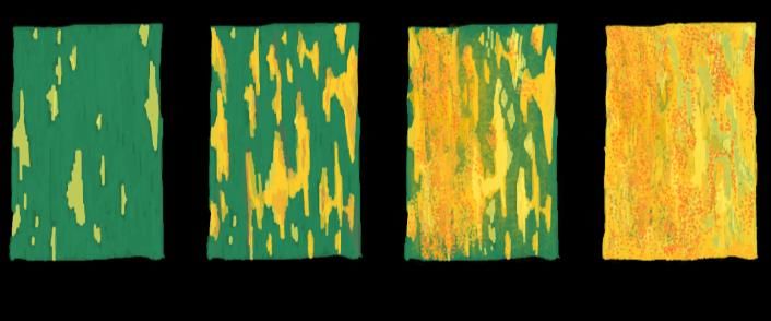
Figure 8 is the methodological flow chart outlining the process of data acquisition,
processing, and analysis. The following section describes the data and steps more in
detail.

3.3 Data

Yellow Rust Incidence Data
Yellow rust incidence data was attained from the International Maize and Wheat
Improvement Center (CIMMYT) Ethiopia. The original data set contained 4,342
yellow rust observation points over three years (2016–2018) across the country
recorded at different wheat growth stages - Tiller, Boot, Heading, Flowering, Milk,
Dough, and Maturity. This study's geographic scope is limited to the Oromia Region,
and the analysis is on the yellow rust cases in the early stage of wheat rust in relation
to pre-seasonal environmental conditions. Therefore, only the observations from the
Oromia Region at Tiller and Boot stage were filtered. In total, 258 observations from
2016 to 2018 were made available for the analysis (Table 1).

Table 1: Yellow rust incidence data used in the study
 Yellow Rust Incidence None (0) Low Moderate High Total
 (Tiller and Boot) (less than 20%) (20-40%) (more than 40%) (n=258)
 2016 35 83 9 3 108
 2017 40 26 1 5 71
 2018 32 45 3 3 79

Incidence level is described with an average score of how the disease is visually observed in the field. The
percentage represents the severity of the yellow rust propagation on the leaves according to the rust scoring guide.

RS-based Data on Environmental Condition
Weather (temperature and precipitation) and Normalized Difference Vegetation Index
(NDVI) were used in the analysis as dynamic environmental parameters. In addition,
in this study, elevation, slope, and aspects were also considered as the static
environmental conditions that could influence the off-season survival of yellow rust
pathogens. While NDVI is regarded as a dynamic environmental parameter, the study
also used this to identify a static characteristic of climate zones based on a unique range
of NDVI values. The dynamic and static RS-based products are summarized in Table
2 and Table 3.

 15

Table 2: List of RS-based products for dynamic environmental conditions

 RS Product Spatial res. period Use
 AgERA5 (Temperature) 11 km 2016-2018 Temperature predictor
 variables

 CHIRPS (Precipitation) 5.55 km 2016-2018 Rain-based predictor variables

 NDVI 10-day maximum composite 1 km 2016-2018 NDVI-based predictor
 data (ProbaV) variables

Table 3: List of RS-based products for static environmental conditions
 RS Product Spatial res. period Use
 NDVI 10-day maximum composite 1 km 2016-2018 Common climate zone
 data (ProbaV)

 SRTM-DEM 30m 2000 Elevation, slope, and aspect

AgERA5 (Temperature)
A collection of daily surface meteorological data prepared for environmental and
agricultural modeling. Temperature data is among the multiple parameters made
available. The temperature data (Kelvin) is available from 1979 to 2018 at the
resolution of 0.1° grid (about 11 km) with global coverage. The product is the
aggregation and correction of ECMWF (European Center for Medium-range Weather
Forecast) ERA5 data. ERA stands for ECMWF Re-Analysis, a deterministic climatic,
land, and oceanic climate data at surface level with 30km (0.28215°) spatial resolution.
ERA5 derives from historical observations by multiple satellite sensors into global
estimates using advanced modeling and data assimilation systems. ECMWF ERA5 data
went through spatial scaling down to 0.1° grid with Nearest Neighborhood algorithm,
temporal aggregation to daily time steps, and bias correction based on the finer
topography, land use pattern, and land-sea delineations to arrive at AgERA5. Source:
ECMWF (2020)

CHIRPS (Precipitation)
A Quasi-global rainfall data set is available over 30 years at 0.05° grid (5.55 km)
resolution. CHIRPS has been developed since 1999 by the U.S. Geological Survey
Earth Resources Observation and Science Center, initially to support the United States

 16

Agency for International Development (USAID)’s Famine Early Warning System
Network (FEWS NET) in collaboration with the National Aeronautics and Space
Administration (NASA) and the National Oceanic and Atmospheric Administration
(NOAA). The product is derived through: rainfall estimates by the infrared Cold Cloud
Duration (the measurement of the threshold at which clouds become precipitation),
long-term historical in-situ observation data, and existing gauge observations for bias
correction. In Ethiopia, CHIRPS products are commonly used in the analysis of
precipitation anomalies, drought, and food insecurity. Reference: Funk et al. (2015)

Note: Relative humidity is another commonly used climate parameter in the study of
rust propagation. However, currently available humidity data was at the resolution of
27km (Global Forecast Systems) or 17km (UK Met Unified Model). This spatial
resolution was considered not adequate for the analysis since many rust observations
spread within the space of 1 to 5 km (many observation points would end up having the
same relative humidity value). The literature review suggests that relative humidity
becomes essential at the time of germination to sporulation of the rust but not
concerning the off-season survival of the already germinated or sporulated lesion of
yellow rust (Tollenaar and Houston, 1967, Eversmeyer and Kramer, 1998). Hence this
variable was not included in this study.

Normalized Difference Vegetation Index (NDVI)
A vegetation index is calculated by comparing the visible and near-infrared sunlight
reflected by the surface. NDVI layers entail the maximum value (range: -0.08 - 0.9) out
of 10 individual images taken over ten sequential days at 1km spatial resolution with
the geographic projection WGS84 (EPSG:4326). The data were generated by the
Global Land Service of Copernicus, the Earth Observation program of the European
Commission in Digital Number (DN) through PROBA-V daily top-of-atmosphere orbit
reflectance values (BRDF-adjusted; Release-Candidate #3 produced by VITO). The
retrieved images were processed to obtain their long-term median data by dekad
between 1999 and 2018 (20 years) to create the 36 dekad specific “normal” data series.
NDVI physical values (PhyVal) are usually generated using DN value, scale factor, and
offset (VITO, 2019).

 ℎ = ∗ 0.004 ( ) − 0.08 ( )
 17

In this study, NDVI was used as an environmental variable potentially associated with
yellow rust incidence. Also NDVI was used to subset the yellow rust observation data
by a unique climate zone. (See 3.4 Data Processing, Data Sub-setting)

DEM
Shuttle Radar Topography Mission (SRTM) Digital Elevation Model (DEM) from the
NASA was used as altitudes and to generate additional terrain characteristics such as
slope and aspect (orientation of slope). SRTM DEM comes in WGS84 Datum and
30m/90m (USGS) spatial resolution.

3.4 Data Processing

Yellow Rust Incidence Categories
Yellow rust incidence was recorded in four levels: None (0), Low (1), Moderate (2),
and High (3). The study initially aimed to assess all four levels of incidence to compare
the probability of different yellow rust incidence levels. However, among the
observations, the Moderate and High incidence was minimal. Thus, the study used a
binary category of yellow rust (0, absent) and yellow rust (1, present) (which includes
low to high incidence).

Retrieval and Processing of Weather Data
AgER5 and CHIRPS data were accessed through Google Earth Engine (GEE) using the
point feature (.shp) generated with the yellow rust observation data from CIMMYT.
The daily values for the period of April-September, 2016-2018, were extracted through
GEE and tabulated using Python and R to calculate the dekad (10-day) maximum,
minimum, and mean temperature; dekad sum of precipitation; and dekad number of
rainy days (>3mm). The Javascript used for the point-based extraction of AgERA5 and
CHIRPS data is available in the Appendices.

A ‘dekad’ approach for dynamic environmental variables
Of all the RS-based data retrieved for temperature, precipitation, and NDVI, variables
for modeling were generated for the period between April and September. April is a

 18

few months before the wheat cropping season begins in Ethiopia. September is where
some tiller-level observations were still observed in rust data each year. Earlier rust
prediction models typically applied monthly intervals or rolling averages over 10, 20,
30, and 60 days for those dynamic variables. However, in this study, 10-day (dekad)
was applied to align the NDVI data interval and was prepared as a 10-day maximum
composition. A dekad is a period of ten days typically used in weather and vegetation
analysis. For example, the first dekad of January is from 1st to 10th January. The second
dekad is from 11th to 20th January, and the third dekad is from 21st to 31st January (the
third dekad in the month with the 31st day contains 11 days). In this study, the dekad
numbering was done annually from the beginning of January till the end of December
(dekad 1 to 36). The analyses focused on the data from the dekad 10 (1-10 April) to the
dekad 27 (21-30 September). Each dekad measure was considered as a dynamic
environmental condition that represents a certain point in time.
Precipitation, temperature, and NDVI are dynamic variables that change over time.
Meanwhile, elevation (DEM), slope, and aspect are considered as static environment
variables. Table 4 below is the list of dynamic and static variables prepared based on
the data from AgERA5 (temperature), CHIRPS (precipitation), NDVI, and SRTM
(elevation, slope, aspect). A total of 111 variables were initially taken into consideration.

Table 4: Environmental variables and description
 Variable Code Description
 prc_mm_10 ~ prc_mm_27 Accumulated precipitation (mm) per dekad

 daysr_10 ~ daysr_27 The number of rainy days with more than 3mm precipitation

 maxT_10 ~ maxT_27 Maximum temperature in dekad (℃)
 minT_10 ~ minT_27 Minimum temperature in dekad (℃)
 meanT_10 ~ meanT_27 Average temperature in dekad (℃)
 ndvi_10 ~ ndvi_27 10-day vegetation density (DN-value)
 DEM Elevation (m)
 Slope Degree of slope
 Aspect Compass direction that slope faces.
 0 = North, 90 = East, 180 = South, 270 = West

 19

Data sub-setting

The rust observation data prepared for this study contains the observations from tiller
and boot level from all over Oromia. Different climate zones, growth levels (tiller or
boot), or even observation timing could have distinct characteristics in the relationship
with environmental variables, hence yields a better model. Therefore, the original data
was further subset into the tiller-only data set, and Climate Zone b data set.

The variability of climate zones was determined based on the unique characteristics of
NDVI propagation over time (through ISODATA pixel clustering), shared across the
observation points. Of five major climate zones (a, b, e, h, j) identified (Figures 9 and
10), the study used the Climate Zone b data set, which had more than 100 observations.

 Figure 9: NDVI profile by group (climate zone)

 20

Figure 10: Map of major climate zones in Oromia Region
 Major climate zones share similar NDVI signatures, and they were identified based on the
 yellow rust observation points. The zones with more than 20 observation points (a, b, e, h,
 and j) were mapped as major climate zones.

After all, three sets of data: mydata, mydata.till, and zone.b were used in the analysis
(Table 5).

Table 5: Three data sets prepared for the analysis
 Observations
 Dataset Description (n= total, [0] = no rust, [1] = rust)
 mydata Tiller and boot level observations. n = 258
 [0] 95, [1]163
 mydata.till Tiller-level yellow rust observations. n = 159
 [0] 75, [1] 84
 zone.b Climate Zone b, tiller and boot level n = 111
 observations. [0] 28 , [1]83

 21

3.5 Analysis
Initially, the weather data was explored to understand the seasonal weather variability
and crop growing seasons around the locations of rust observations in the Oromia
Region. Subsequently, using the tabulated data sets, analyses were conducted to address
the three Research Questions (RQs) designed for this study (Figure 8: Methodological
Flowchart - Analysis). The scripts used in the analyses are available in Appendices.

 3.5.1 Variable Exploration (RQ1.a)

Research Question 1.a (RQ1.a) probes the association between yellow rust incidence
and environmental conditions. The RS-based 111 environmental variables (temperature,
precipitation, NDVI, and terrain characteristics) were examined against yellow rust
observations in the three data subsets: mydata, mydata.till, and zone.b. The objective
here was to understand what types of variables are more associated with yellow rust
and narrow down the number of related variables. A combination of univariate
correlation analysis and Classification Tree (CT) analysis were applied.

Univariate correlation:

When there are multiple variables in hand, Area Under ROC Curve (AUC) helps
identify the more relevant ones than the others. Especially when the response variable
(rust incidence) is categorical (i.e., incidence or no-incidence), AUC quantifies the
extent to which the respective variable can separate these two categories. An AUC score
of around 0.5 is an indication of a completely irrelevant variable. The R.
package ‘caret’ was used to calculate AUC for each variable. AUC values were
calculated by k-fold cross validation that enabled several repetitions of AUC value
calculation. By averaging multiple cycles of AUC calculation, the AUC values
presented were made more reliable. AUC helps identify the variables that are
individually associated with yellow rust infection. However, this does not address
interactions between different variables that may create an environment conducive to
potential off-season survival of pathogen and impact early infection at the tiller/boot-
level.

 22

Classification Tree (CT):

CT was applied to identify a small number of variables that serve as good predictors. It
categorizes the observation data into smaller and homogeneous groups by repeating a
binary splitting based on the influential predictors (Hastie et al., 2009). This splitting
aims to categorize the observation data, for example, in the case of yellow rust,
into infected or not infected based on the influencing factors such as temperature and
precipitation. Initially, the data categorized as infected may contain some uninfected
observations, but this ‘impurity’ minimizes as splitting is repeated multiple times to
better categorize the classes. The resulting summary of all the splitting forms a tree-like
shape. Practically, CT is a modeling process on its own, but this was used purely for
variable exploration and reducing the number of potential environmental variables in
this part of the analysis. CT was undertaken using the ‘cart’ package in R.

The variables were analyzed group-wise: maxT, minT, meanT, prc_mm, daysr, ndvi,
and terrain (DEM, slope, aspect). The top-performing variables from each variable
group were put together to find out the combination variables that achieved the lowest
relative errors, and cross-validation errors were grouped as the variables most
associated with the rust and forwarded to the next step to address RQ1.b.

 3.5.2 Finding the most critical variables (RQ1.b)

The study applied General Additive Model (GAM) and Boosted Regression Model
(BRT) to understand more about the critical variables associated with the early yellow
rust incidence. Datasets were randomly split into training data (70%) for model training
and test data (30%) for model evaluation using the R package ‘caret’. This part of the
analysis essentially builds models that explain the interaction of different
environmental variables related to yellow rust incidence. The best performing models
were forwarded to address the subsequent Research Question 2.

GAM

GAM (Hastie et al., 2009) is a progression of the Generalized Linear Model (GLM,
Nelder and Wedderburn (1972)) which had considered the response variable that are
not-normally distributed. GAM enhances GLM by considering nominal/categorical and

 23

ordinal predictors in their characteristics and maximizing a model's prediction capacity
(Ravindra et al., 2019). While the ordinary regression model fits simple least-squares
as function, GAM model fitting is based on the ‘smoothing’ function using a scatterplot
smoother such as cubic smoothing spline or kernel smoother (Hastie et al., 2009). The
smoothing function takes into consideration the nature of predictive variables that are
not normally distributed. Thus, GAM is a flexible statistical method for identifying and
characterizing nonlinear regression effects (Hastie et al., 2009).

With a random variable and a set of the predictor variable 1 , 2 , … , , a
regression model estimates ( | 1 , 2 , … , ) . The formula for a traditional
regression model like GLM is expressed as:

 ( | 1 , 2 , … , ) = 0 + 1 1 + … + 

where 0 , 1 , … , are generated by least squares. Meanwhile, GAM assumes the
following formula:
 
 ( | 1 , 2 , … , ) = 0 + ∑ ( )
 =1

where (. )’s are smooth functions that are estimated through a scatterplot smoother.
The details of how scatter smoothers work are available by Hastie and Tibshirani (1986).

To the best of the author’s knowledge, GAM has not been applied in yellow rust
modeling. However, this has been widely used in many other fields, such as in plant
ecology (Yee and Mitchell, 1991), species habitat study (Suárez-Seoane et al., 2002),
and environmental health (Bouzid et al., 2014). The R package ‘mgcv’ was used in
GAM analysis. GAM has a function called ‘smoothing’ or ‘splines’ to realize flexible
non-linear expression. In R. package ‘mgcv’, this smoothness can be defined by the user
or automatically suggested by setting the method with Restricted Maximum Likelihood
(REML).

Some of the methods to understand model convergences are:

 i. summary() for model statistics to check parametric coefficient and significance
 of smooth terms

 ii. plogis() to transform the model outcome to the log-odds scale to assess the extent
 of the model’s prediction of a positive outcome (i.e., yellow rust infection).

 24

iii. plot() to visualize the partial effect of the concerned variables with a confidence
 interval.

 iv. gam.check() to check the random distribution of residuals for each predictor
 variable. “Basis function” (this influences the smooth parameter) for variables is
 adjustable to improve the model performance.

 v. Collinearity and Concurvity check

 Collinearity is the correlation among the predictors that potentially influence the
 model convergence. ggpairs() in the ‘GGally’ package was used to plot the
 variable interactions. Variance Inflation Factor (VIF) calculation was also
 conducted to decide which variable to drop.

 Concurvity is when one variable smooth term in GAM is approximated by one or
 more other variable smooth terms. Even though the variables are not collinear,
 concurvity can occur. The function concurvity() was used to check and rule out
 potential concurvity.

BRT

BRT (Friedman, 2001) is a combination of statistics and machine learning, guided by
an algorithm to achieve the most optimal model (Youssef et al., 2016). BRT’s rule sets
are two-fold: “classification/regression trees” to find the most influential predictors;
and “boosting” to synthesize many possible models to build the best performing model
(Elith et al., 2008, Schapire, 2003).

There are four parameters that need to be set and adjusted to maximize the resulting
model performance.

 i. learning rate (lr): signifies the contribution of each tree to the final fitted model;

ii. tree complexity (tc): the number of total nodes (split point) in the tree;

iii. number of trees (nt): the result of lr and tr; and

iv. bag fraction (bf): the portion of data to be used for each iteration.

 25

BRT can be applied to data that is not-normally distributed, and it is widely used in
ecological and environmental model building (Naghibi et al., 2016, Pittman and Brown,
2011, Zellweger et al., 2013). BRT can select only relevant variables and ignore non-
informative predictors. However, as Elith et al. (2008) point out, for small datasets
where redundant predictors may degrade performance by increasing variance, it is
better to simplify the list of predictor variables in advance instead of putting them all at
once into the model. Thus, only the pre-selected list of predictor variables from RQ1.a
was used in BRT. The R package ‘dismo’ and ‘gbm.step’ were used in BRT analysis.

In R, gbm.step() uses cross-validation (default k=10) to estimate the optimal number of
trees. Considering the relatively small sample size (number of observations) used in the
analysis, tree complexity (tc) 2 and learning rate (lr) 0.001 were used, unless a smaller
lr yielded better models.

Model statistics in summary() and gbm.plot() report were examined to understand the
relative importance/influence of key environmental variables. Tree Complexity (tc) and
Learning Rate (lr) were as necessary to achieve better model statistics.

gbm.interactions() was used to understand the interactions between the critical
environmental variables, and gbm.perspec() was used to visualize the interactions.

 3.5.3 Assessing Model Predictive Capacity (RQ2)

Research Question 2 (RQ2) examines how reliably the RS-based environmental
predictors can project yellow rust incidence among young wheat. The trained GAM and
BRT models were used to predict yellow rust incidence using the test data (30% of
observations). The R. package ‘mgcv’ and ‘gbm’ were used to conduct prediction.

The output of model prediction is in the form of probability with the values ranging
from 0 to 1. This value was classified into 0 (probability < 0.5) and 1 (probability >=
0.5) in order to compare with the actual incidence of yellow rust.

A confusion matrix (Figure 11) was created with the prediction and actual observation.

 26

Prediction

 0 1

 Actual Observation
 True False
 Negative Positive 0
 (TN) (FP)

 False True
 Negative Positive 1
 (FN) (TP)
 Figure 11: Confusion Matrix

On R., a function ModelPerformance() was used to examine the key statistics to assess
the GAM and BRT models' predictive performance. These statistics include Accuracy,
Kappa Statistic, Sensitivity, Specificity, and Precision.

 a. Accuracy is the ratio of correct predictions calculated by the true positive (TP)
 and true negative (TN) divided by the total number of events.

 + 
 =
 + + + 

 b. Kappa Statistic (Cohen, 1960): the extent to which prediction and observations
 agree with the actual yellow rust incidence

 − 
 =
 1 − 

 where is the relative observed agreement, and is the hypothetical
 probability of chance agreement.

 + 
 =
 + + + 
 + + 
 = ( ∗ )
 + + + + + + 
 + + 
 + ( ∗ )
 + + + + + + 

 Kappa statistic Level of agreement
 ≦0 no agreement
 0.01 – 0.20 none to slight agreement

 27

0.21 – 0.40 fair agreement
 0.41 – 0.60 moderate agreement
 0.61 – 0.80 substantial agreement
 0.81 – 1.00 almost perfect agreement

 c. Sensitivity is a true positive (TP) rate. It measures the rate of actual yellow rust
 cases corrected (predicted yellow rust case is an incidence in the observation)

 =
 + 

 d. Specificity is a true negative (TN) rate. It measures the rate of the negatives
 correctly predicted (the predicted no-yellow rust case is the no-yellow rust in
 the real observation data)

 =
 + 

 e. Precision is how accurately the model predicted the positive cases

 =
 + 

 3.5.4 Model Extrapolation over Oromia Region

The models with good predictive performance were used to extrapolate the yellow rust
probabilities (in the scale of 0 – 1) over wider areas of interest. The maps were
generated for 2016, 2017, and 2018, respectively. The key environmental variables
from the identified dekad period (for dynamic variable) were re-generated as raster
layers from the respective sources (AgER5, CHIRPS ProbaV NDVI, and STRM DEM)
of RS products. The R scripts used in the extrapolation are available in Appendices.

 28