Understanding and improving model representation of aerosol optical properties for a Chinese haze event measured during KORUS-AQ - ACP
←
→
Page content transcription
If your browser does not render page correctly, please read the page content below
Atmos. Chem. Phys., 20, 6455–6478, 2020
https://doi.org/10.5194/acp-20-6455-2020
© Author(s) 2020. This work is distributed under
the Creative Commons Attribution 4.0 License.

Understanding and improving model representation of aerosol
optical properties for a Chinese haze event measured
during KORUS-AQ
Pablo E. Saide1,2 , Meng Gao3 , Zifeng Lu4 , Daniel L. Goldberg4 , David G. Streets4 , Jung-Hun Woo5 ,
Andreas Beyersdorf6 , Chelsea A. Corr7 , Kenneth L. Thornhill8,18 , Bruce Anderson8 , Johnathan W. Hair8 ,
Amin R. Nehrir8 , Glenn S. Diskin8 , Jose L. Jimenez9 , Benjamin A. Nault9 , Pedro Campuzano-Jost9 , Jack Dibb10 ,
Eric Heim10 , Kara D. Lamb11 , Joshua P. Schwarz11 , Anne E. Perring12 , Jhoon Kim13 , Myungje Choi13,14 ,
Brent Holben15 , Gabriele Pfister16 , Alma Hodzic16 , Gregory R. Carmichael17 , Louisa Emmons16 , and
James H. Crawford8
1 Department    of Atmospheric and Oceanic Sciences, University of California – Los Angeles, Los Angeles, CA, USA
2 Institute of the Environment and Sustainability, University of California – Los Angeles, Los Angeles, CA, USA
3 Department of Geography, Hong Kong Baptist University, Hong Kong SAR, China
4 Energy Systems Division, Argonne National Laboratory, Lemont, IL 60439, USA
5 Department of Technology Fusion Engineering, Konkuk University, Seoul, South Korea
6 Department of Chemistry & Biochemistry, California State University San Bernardino, San Bernardino, CA, USA
7 USDA UV-B Monitoring and Research Program, Natural Resource Ecology Laboratory,

Colorado State University, Fort Collins, CO, USA
8 NASA Langley Research Center, Hampton, VA, USA
9 Department of Chemistry, and Cooperative Institute for Research in Environmental Sciences,

University of Colorado, Boulder, CO, USA
10 Institute for the Study of Earth, Oceans, and Space, University of New Hampshire, Durham, NH, USA
11 Chemical Sciences Laboratory, Earth System Research Laboratories, Boulder, CO, USA
12 Department of Chemistry, Colgate University, Hamilton, NY, USA
13 Department of Atmospheric Sciences, Yonsei University, Seoul, 03722, Korea
14 Jet Propulsion Laboratory, California Institute of Technology, Pasadena, CA 91109, USA
15 NASA Goddard Space Flight Center, Greenbelt, Maryland, USA
16 Atmospheric Chemistry Observations and Modeling Lab, National Center for Atmospheric Research, Boulder, CO, USA
17 Center for Global & Regional Environmental Research, University of Iowa, Iowa City, Iowa, USA
18 Science Systems and Applications Inc., Hampton, VA USA

Correspondence: Pablo E. Saide (saide@atmos.ucla.edu)

Received: 5 November 2019 – Discussion started: 25 November 2019
Revised: 15 April 2020 – Accepted: 4 May 2020 – Published: 4 June 2020

Abstract. KORUS-AQ was an international cooperative air          tion captured AOD during this pollution episode but overpre-
quality field study in South Korea that measured local and re-   dicted surface particulate matter concentrations in South Ko-
mote sources of air pollution affecting the Korean Peninsula     rea, especially PM2.5 , often by a factor of 2 or larger. Anal-
during May–June 2016. Some of the largest aerosol mass           ysis revealed multiple sources of model deficiency related to
concentrations were measured during a Chinese haze trans-        the calculation of optical properties from aerosol mass that
port event (24 May). Air quality forecasts using the WRF-        explain these discrepancies. Using in situ observations of
Chem model with aerosol optical depth (AOD) data assimila-       aerosol size and composition as inputs to the optical prop-

Published by Copernicus Publications on behalf of the European Geosciences Union.
6456                  P. E. Saide et al.: Understanding and improving model representation of aerosol optical properties

erties calculations showed that using a low-resolution size        aerosol mass to optical properties is performed in these mod-
bin representation (four bins) underestimates the efficiency       els, often showing large inter-model variability (Myhre et al.,
with which aerosols scatter and absorb light (mass extinction      2013; Stier et al., 2013; Kipling et al., 2016). Similarly, short-
efficiency). Besides using finer-resolution size bins (8–16        term predictions of solar power (Schroedter-Homscheidt et
bins), it was also necessary to increase the refractive indices    al., 2013; Jimenez et al., 2016) and visibility forecasts (Clark
and hygroscopicity of select aerosol species within the range      et al., 2008; Lee et al., 2017) also require the use of aerosol
of values reported in the literature to achieve better consis-     optical properties. Thus, evaluating the ability of models to
tency with measured values of the mass extinction efficiency       properly translate aerosol mass and number concentrations
(6.7 m2 g−1 observed average) and light-scattering enhance-        into aerosol optical properties is key to providing confidence
ment factor (f (RH)) due to aerosol hygroscopic growth (2.2        in model results supporting these disciplines.
observed average). Furthermore, an evaluation of the opti-            Previous research has shown various degrees of consis-
cal properties obtained using modeled aerosol properties re-       tency between model evaluations of surface aerosol mass
vealed the inability of sectional and modal aerosol represen-      concentrations and column-integrated aerosol properties. Lee
tations in WRF-Chem to properly reproduce the observed             et al. (2016) used satellite AOD to constrain surface PM10
size distribution, with the models displaying a much wider         (particulate matter with diameters below 10 µm) predictions
accumulation mode. Other model deficiencies included an            and found large improvements against surface monitors re-
underestimate of organic aerosol density (1.0 g cm−3 in the        gardless of the model used for aerosol optical properties.
model vs. observed average of 1.5 g cm−3 ) and an overpre-         Their results also showed slight discrepancies in the PM10
diction of the fractional contribution of submicron inorganic      and AOD when comparing models to observations, with
aerosols other than sulfate, ammonium, nitrate, chloride, and      some optical models showing larger biases in PM10 than
sodium corresponding to mostly dust (17 %–28 % modeled             AOD and some presenting the opposite behavior. Lennart-
vs. 12 % estimated from observations). These results illus-        son et al. (2018) also found discrepancies when compar-
trate the complexity of achieving an accurate model repre-         ing the ratio between PM2.5 and AOD for observations and
sentation of optical properties and provide potential solutions    WRF-Chem simulations; the modeled ratios were 30 %–
that are relevant to multiple disciplines and applications such    50 % higher over South Korea during May–June 2016. Simi-
as air quality forecasts, health impact assessments, climate       lar discrepancies were found by Mangold et al. (2011) when
projections, solar power forecasts, and aerosol data assimila-     assessing model skill in predicting a regional pollution event
tion.                                                              over Europe driven by forest fire emissions and stagnation.
                                                                   Crippa et al. (2019) performed an ensemble of simulations
                                                                   to assess what combination of model inputs and configu-
                                                                   rations resulted in the best agreement with observations in
1   Introduction                                                   the southeast US. They reported that simulations configured
                                                                   with a modal aerosol model performed the best against AOD
Exposure to air pollutants is estimated to be the leading          observations, while a sectional aerosol approach showed the
environmental risk affecting human health (Gakidou et al.,         best agreement against surface PM2.5 , and hypothesized that
2017), and aerosols represent the leading pollutant responsi-      aerosol hygroscopic growth and optical properties calcula-
ble for these effects (Cohen et al., 2017). The estimates of       tions could play a role in this discrepancy. Palacios-Peña et
aerosol impacts on human health generally involve the use of       al. (2019) evaluated the aerosol optical properties of an en-
ground-based monitoring networks that are combined with            semble of models over Europe, finding that differences due
aerosol optical depth (AOD) satellite retrievals and/or model      to diversity in modeling systems were larger than when using
estimates for regions not monitored to obtain global esti-         different emission inventories or when turning aerosol radia-
mates (Liu et al., 2009; van Donkelaar et al., 2016; Goldberg      tive feedbacks on and off. Reddington et al. (2016) evalu-
et al., 2019a). The use of AOD to estimate surface concentra-      ated a global aerosol model in tropical regions affected by
tions often involves using atmospheric composition simula-         biomass burning. They found that the model underestimated
tions able to “translate” a column-integrated measure of light     AOD more than PM2.5 , even when an upper-limit estimate of
extinction due to aerosols (AOD) into surface aerosol mass         aerosol hygroscopicity was assumed for the aerosols. Red-
concentrations. Satellite AOD is also often used to improve        dington et al. (2019) found further inconsistencies, as the
air quality forecasts of surface particulate matter through data   model showed a good representation of the observed verti-
assimilation (Saide et al., 2013, 2014; Kumar et al., 2019;        cal profile while underestimating AOD, and hypothesized it
Benedetti et al., 2009). Aerosols also impact climate through      was due to uncertainties in the AOD computations. In another
aerosol–cloud–radiation interactions and represent one of the      study, Zieger et al. (2013) compared observations of scatter-
largest uncertainties in climate projections (Boucher et al.,      ing enhancement due to hygroscopic growth against results
2013). Chemistry–climate models estimate 3-D distributions         from the Optical Properties of Aerosols and Clouds (OPAC)
of aerosols, which are used by a radiative transfer module to      software module, showing a systematic overprediction. This
estimate aerosol radiative effects. Again, this translation of     overprediction could lead to mismatches between AOD and

Atmos. Chem. Phys., 20, 6455–6478, 2020                                              https://doi.org/10.5194/acp-20-6455-2020
P. E. Saide et al.: Understanding and improving model representation of aerosol optical properties                         6457

PM2.5 in models using this code. Curci et al. (2019) evaluated   were scaled differently. Although there was no data assimi-
black carbon absorption for an ensemble of models over Eu-       lation performed on the inner domain, this domain was ini-
rope and North America, finding that biases were driven by       tialized 18 h after the outer domain and was thus influenced
the mixing state assumptions in the optical properties com-      by data assimilation through initial and boundary conditions.
putations.                                                       The forecast configuration was based on WRF-Chem ver-
   The KORUS-AQ (Korea–United States Air Quality) cam-           sion 3.6.1 with modifications. The aerosol and gas chemistry
paign was an international cooperative air quality field study   packages corresponded to the four-size-bin Model for Simu-
in South Korea that measured local and remote (e.g., anthro-     lating Aerosol Interactions and Chemistry (MOSAIC; Zaveri
pogenic, biomass burning, dust) sources of air pollution af-     et al., 2008) and a simplified hydrocarbon chemical mecha-
fecting the Korean Peninsula during May–June 2016. The           nism (Pfister et al., 2014), both selected to reduce computa-
objectives of the present study are to (1) evaluate one of the   tional costs compared to using the eight-size-bin MOSAIC
forecast systems used to support flight planning during the      configuration and more complex chemical mechanisms. Al-
mission; (2) assess the degree of consistency between aerosol    though detailed secondary organic aerosol (SOA) forma-
optical properties and mass concentrations for the forecast-     tion schemes have been implemented for the four-bin MO-
ing and other configurations; and (3) explain the identified     SAIC configuration (Shrivastava et al., 2013; Knote et al.,
discrepancies. The results will provide guidance for future      2015), it increases computational costs significantly. Thus,
model development and we expect will motivate this type of       the simplified SOA formation scheme, proposed by Hodzic
analysis for other modeling systems and locations.               and Jimenez (2011) and verified to work well in multiple
                                                                 later studies (e.g., Hayes et al., 2015; Shah et al., 2019), was
                                                                 implemented to keep computational costs low. While this
2     Methods                                                    scheme included anthropogenic and biomass burning SOA,
                                                                 biogenic SOA was also modeled by using an SOA precur-
2.1    Regional modeling                                         sor surrogate derived from isoprene as described in Shrivas-
                                                                 tava et al. (2011). Aerosol–radiation interactions were in-
Air quality forecasts were performed using the Weather Re-       cluded (Fast et al., 2006), while aerosol–cloud interactions
search and Forecasting model (Skamarock et al., 2008) cou-       were excluded to avoid the computational costs of track-
pled to Chemistry (WRF-Chem) (Grell et al., 2005) to sup-        ing cloud-borne aerosols. Anthropogenic emissions were de-
port both KORUS-AQ flight planning and post-campaign             veloped by Konkuk University for KORUS-AQ forecasting
analysis. The modeling domains are shown in Fig. 1, with a       and are described in Choi et al. (2019a) and Goldberg et
regional domain of 20 km resolution, covering major source       al. (2019b). Natural dust, sea spray, and biogenic emissions
regions of transboundary pollutants affecting the Korean         were computed online using the Goddard Aerosol Radiation
Peninsula: anthropogenic pollution from eastern China, dust      and Transport (GOCART) scheme (Ginoux et al., 2001; Zhao
from inner China and Mongolia, and wildfires from Siberia        et al., 2010), following Gong et al. (2002), and estimates
(Saide et al., 2014). A 4 km resolution domain was nested to     from the Model of Emissions of Gases and Aerosol from Na-
cover the Korean Peninsula and surroundings at higher res-       ture (MEGAN; Guenther et al., 2006), respectively. Biomass
olution. This inner domain encompassed the region where          burning emission estimates were obtained from the Quick
the KORUS-AQ flights were planned and was able to bet-           Fire Emissions Dataset (Darmenov and da Silva, 2015) and
ter resolve local sources. The forecasts were performed once     were added using the online plume-rise model implemented
daily and used meteorological initial and boundary condi-        in WRF-Chem (Grell et al., 2011). Other modeling configu-
tions from the National Centers for Environmental Predic-        rations related to meteorological parameterizations and anal-
tion Global Forecast System (NCEP, 2007) and chemical            ysis nudging are described in Saide et al. (2014).
boundary conditions from the Copernicus Atmosphere Mon-             In addition to the forecasting results, we performed retro-
itoring Service (Inness et al., 2015). Initial conditions for    spective sensitivity simulations summarized in Table 1. We
gases and aerosols were obtained from the previous fore-         first used the same configuration as the forecast, which we
casting cycle. AOD data assimilation was implemented for         labeled MOSAIC4b. To explore the model sensitivity to in-
the outer domain using data from low-earth-orbiting (GMAO        creasing the resolution of the aerosol size bins, we performed
Neural Network retrieval) and geostationary satellites (Geo-     simulations using the MOSAIC eight-bin configuration cou-
stationary Ocean Color Imager retrievals; Choi et al., 2016,     pled to the Carbon Bond Mechanism version Z (CBM-Z)
2018; Lee et al., 2010) as described in Saide et al. (2014).     chemical scheme (Zaveri and Peters, 1999) and labeled it
To our knowledge, this was the first near-real-time imple-       MOSAIC8b. Some caveats of this sensitivity simulation are
mentation of assimilating geostationary AOD. Each assimila-      that it uses a different gas-phase chemistry scheme and does
tion step modified aerosol mass, keeping the species distribu-   not include secondary organic aerosol formation; thus, this
tion and size of each bin constant. Thus, the assimilation had   needs to be considered in the analysis when comparing it
the potential to change the bin-aggregated composition and       to the base configuration. WRF-Chem can also be config-
size distribution when size bins with different compositions     ured with the Modal Aerosol Dynamics Model for Europe

https://doi.org/10.5194/acp-20-6455-2020                                          Atmos. Chem. Phys., 20, 6455–6478, 2020
6458                   P. E. Saide et al.: Understanding and improving model representation of aerosol optical properties

Table 1. Summary of WRF-Chem simulations. Refractive indices, hygroscopicity parameters, and size bins are defined in Tables 2 and 3.
Refer to Sect. 3.2 and 3.3 for definitions of the base and updated configurations.

         Name           Aerosol scheme         Size bins used for OP   GSD of the modes     Refractive index   Hygroscopicity
         MOSAIC4b       Sectional four bins    Four bins               –                    Base               Base
         MOSAIC8b       Sectional eight bins   Eight bins              –                    Base               Base
         MADE1          Modal                  Eight bins              Base                 Base               Base
         MADE2          Modal                  Eight bins              Updated              Base               Base
         MADE3          Modal                  Eight bins              Updated              Updated            Base
         MADE4          Modal                  Eight bins              Updated              Updated            Updated

                                                                       black carbon and other inorganics (OINs; inorganic aerosols
                                                                       other than sulfate, ammonium, nitrate, chloride, and sodium)
                                                                       are considered to absorb solar radiation with an imaginary
                                                                       refractive index of 0.71 and 0.006, respectively. For the MO-
                                                                       SAIC configurations, the size bins in the optical properties
                                                                       calculation correspond to those in the aerosol model (four
                                                                       and eight size bins, defined in Table 3), while for modal
                                                                       aerosols the modes are mapped to eight sectional bins (the
                                                                       same boundaries as the eight MOSAIC bins) before the cal-
                                                                       culation by computing the aerosol mass and number concen-
                                                                       tration included in each section. WRF-Chem computes op-
                                                                       tical properties for ambient conditions. Thus, the derivation
Figure 1. Modeling domains for the forecast simulations. Only the      of dry extinction and scattering enhancements due to hygro-
outer domain is used for the retrospective simulations.                scopic growth at fixed relative humidity requires computa-
                                                                       tions at the post-processing stage. These computations re-
                                                                       quire the aerosol water to be recalculated for the specified rel-
(MADE) model, whereby aerosol sizes are represented by                 ative humidity. Since both the MOSAIC and MADE aerosol
lognormal modes (as opposed to sections as for MOSAIC).                models compute aerosol water based on aerosol thermody-
We used the configuration coupled to the updated Regional              namics, versions of these computations are needed at the
Atmospheric Chemistry Mechanism (RACM; Ahmadov et                      post-processing stage. In order to simplify the process and
al., 2015), which contains secondary organic aerosol forma-            add additional capabilities, an alternative optical properties
tion using the volatility basis set (Ahmadov et al., 2012) and         code at the post-processing stage was developed that mimics
aerosol optical properties calculations (Tuccella et al., 2015).       the WRF-Chem one. This alternative approach uses Mie cal-
We label these simulations as MADE plus a number, with                 culations from the Mätzler (2002) code, which is based on
the number going from 1 to 4 depending on changes to the               the Appendix of Bohren and Huffman (1983). Aerosol water
parameters described in Table 1.                                       uptake was parameterized using the method proposed by Pet-
   Simulations MOSAIC4b, MOSAIC8b and MADE1 are re-                    ters and Kreidenweis (2007), which utilizes the hygroscop-
ferred to as base configurations, while MADE2–4 are sen-               icity parameter (κ). Values for the hygroscopicity parame-
sitivity simulations. All retrospective simulations were per-          ter representing the base configuration are obtained from the
formed only for the 20 km resolution domain in this study, as          WRF-Chem code used to compute aerosol water for the God-
we focus on a pollution event from long-range transport (24–           dard Chemistry Aerosol Radiation and Transport (GOCART;
26 May 2016). Also, no data assimilation was performed for             Chin et al., 2002) model, which implements the κ approach
these simulations. Unless otherwise noted, they use the same           and a volume mixing rule. Following this configuration κ is
inputs and parameterizations as for the forecast simulations.          set to 0.5 for ammonium sulfate and ammonium nitrate. For
                                                                       sodium chloride κ is set to 1.5 (Zieger et al., 2017). For or-
2.2    Optical properties calculation                                  ganic aerosol, black carbon, and dust, κ is set to zero as these
                                                                       aerosol types are currently not considered to be electrolytes
Aerosol optical properties in WRF-Chem are computed us-                in the MOSAIC and MADE thermodynamic models and thus
ing a Mie code and Chebyshev expansion coefficients for                do not contribute to water uptake in these frameworks (Fast et
each size bin, assuming an internal mixture within the bin             al., 2006). Ways to improve these simplifications will be dis-
and a volume mixing rule (Fast et al., 2006). The refractive           cussed later in the text. Figure 2 shows an evaluation of the
indices (real part) and density used for each species are de-          alternative approach against the WRF-Chem routines used in
fined in Table 2 under the base configuration column. Only

Atmos. Chem. Phys., 20, 6455–6478, 2020                                                  https://doi.org/10.5194/acp-20-6455-2020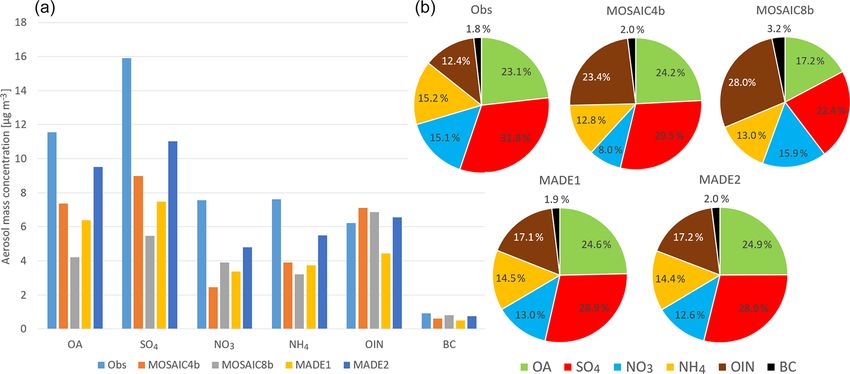
P. E. Saide et al.: Understanding and improving model representation of aerosol optical properties                                           6459

Table 2. Real refractive indexes (dimensionless), hygroscopicity parameter (dimensionless), and aerosol density (g cm−3 ) used in the base
and updated configurations. Values that changed in the updated configurations are noted in italics. Note that measured organic aerosol density
was used in the closure studies.

                                                     Real refractive index    Hygroscopicity parameter       Density
                                                     Base         Updated     Base               Updated        Base
                             Ammonium sulfate        1.52            1.527         0.5               0.61         1.8
                             Ammonium nitrate         1.5            1.553         0.5               0.67         1.8
                             Sodium chloride         1.45             1.45         1.5                1.1         2.2
                             Other inorganics        1.55             1.55           0               0.14         2.6
                             Organic aerosol         1.45             1.55           0               0.14           1
                             Black carbon            1.85             1.85           0                  0           1
                             Aerosol water           1.33             1.33           –                  –           1

Figure 2. (a) Extinction-to-mass ratio for dry conditions (20 % RH) as a function of dry particle diameter considering a monodisperse
aerosol distribution of fixed aerosol composition equal to the mean of the data analyzed. Blue and green lines represent results using optical
properties code from WRF-Chem and the alternative approach, respectively. (b) Scatterplot comparing aerosol water (µg m−3 ) estimated
by WRF-Chem routines for the forecast simulations (MOSAIC four-bin) and using the alternative approach at 80 % RH during 02:00–
05:00 UTC of the flight analyzed in this study. The solid red line indicates the 1 : 1, line and the dashed red line represents the regression line
(slope of 0.94).

post-processing mode for the MOSAIC model that were de-                      using variable density for aerosol species, and altering κ to
veloped as part of the data assimilation scheme (Saide et al.,               vary the extent to which different aerosol chemical species
2013). Under dry conditions, the alternative approach shows                  take up water.
similar results as the WRF-Chem optical properties, with the
extinction-to-mass ratio curves following each other for all                 2.3     Airborne observations
sizes (Fig. 2a). The high-frequency oscillations shown by
the Mie code of our alternative approach are smoothed in                     Airborne data used in this study were measured by instru-
WRF-Chem due to the use of the Chebyshev expansion co-                       ments onboard the NASA DC-8 research aircraft as part of
efficients (Fast et al., 2006) and interpolation between wave-               the KORUS-AQ campaign (Aknan and Chen, 2019) during
lengths (optical properties at 400 and 600 nm are used to de-                the flight starting at 22:00 UTC on 24 May (25 May local Ko-
rive values at mid-visible wavelengths). Water uptake using                  rean time) 2016. This flight focused on measurements over
the MOSAIC approach and the one described here provides                      the Yellow Sea and sampled some of the highest aerosol
similar results (Fig. 2b), with values ∼ 7 % lower in the al-                mass concentrations of the deployment, originating mostly
ternative approach that will be taken into consideration when                from anthropogenic pollution from China (Peterson et al.,
evaluating the optical properties code in the next sections.                 2019; Nault et al., 2018). This flight was also chosen as it
The alternative optical properties code provides flexibility to              corresponds to a period of large model discrepancies (see
evaluate changes in configuration that would be difficult to                 the “Results and discussion” section). Measurements used in
implement in the WRF-Chem optical properties code. These                     this study include numerous in situ chemical compositions,
include using more than eight bins to improve size resolution,               mass concentrations, and physical properties of the aerosol,

https://doi.org/10.5194/acp-20-6455-2020                                                       Atmos. Chem. Phys., 20, 6455–6478, 2020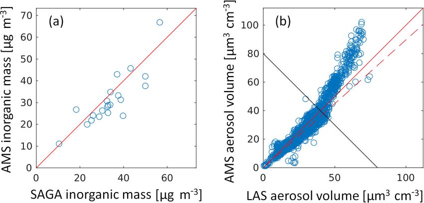
6460                  P. E. Saide et al.: Understanding and improving model representation of aerosol optical properties

as well as remote sensing physical properties of the aerosol.
PM1 , not including black carbon, was measured by the Uni-
versity of Colorado Boulder high-resolution time-of-flight
aerosol mass spectrometer (HR-ToF-AMS, hereinafter AMS
for short; DeCarlo et al., 2006; Nault et al., 2018). These
measurements included the mass concentrations of sulfate,
nitrate, ammonium, chloride, and organic aerosol, as well
as the estimated aerosol density. The estimation of aerosol
density is described in Nault et al. (2018) and DeCarlo et
al. (2004). Refractory black carbon concentrations were mea-
sured by the NOAA Single Particle Soot Photometer (SP2;
Lamb et al., 2018). Bulk water-soluble inorganic aerosol was     Figure 3. (a) Scatterplot of total inorganic aerosol (sulfate, ammo-
                                                                 nium, chloride, and nitrate) mass (µg m−3 ) as measured by SAGA
measured by the University of New Hampshire using Teflon
                                                                 and AMS, averaging the AMS data to the SAGA integration time
filters, followed by offline ion chromatography with an esti-    (R 2 = 0.72, slope = 1.07). The solid red line indicates the 1 : 1 line.
mated aerodynamic diameter cutoff of ∼ 4 µm (SAGA; Dibb          (b) Scatterplot of aerosol volume measured by the AMS and LAS,
et al., 2000; McNaughton et al., 2007). The in situ physi-       accounting for the AMS transmission. The solid red line indicates
cal aerosol properties were measured by the NASA Lang-           the 1 : 1 line, the solid black line represents an approximate cutoff
ley Aerosol Research Group (LARGE), which included dry           for the LAS saturation, and the dashed red line represents the re-
aerosol scattering, extinction and single-scattering albedo,     gression line when using data below the black line (slope of 0.9).
and scattering enhancements due to hygroscopic growth.
These measurements were done with two TSI nephelome-                                    √
ters (at 450, 550, and 700 nm wavelength) and a particle soot    dynamic diameter by X/ρ (valid in the continuum regime
absorption photometer (at 470, 532, and 660 nm wavelength)       where most of the coarse-mode aerosol mass is in this study)
as described in Ziemba et al. (2013). Aerosol size distribu-     and assuming a dynamic shape factor (X = 1.6) and density
tions were also measured by the LARGE suite using a scan-        (ρ = 2.6 g cm−3 ) for dust aerosols, which we assume dom-
ning mobility particle sizer (SMPS, TSI model 3936), a laser     inates the coarse-mode aerosol. This assumption is made as
aerosol spectrometer (LAS, TSI model 3340), and an aerody-       AMS and SAGA measured similar concentrations of inor-
namic particle sizer (APS, TSI model 3321). AMS and SP2          ganic species (Fig. 3a), and thus sulfate, ammonium, chlo-
measure mostly submicron aerosols, while the LARGE inlet         ride, and nitrate were mostly not present in sizes covered by
cutoff is at 5 µm aerodynamic diameter (McNaughton et al.,       SAGA but not by AMS. But since the aerosol size distribu-
2007). Relative humidity was estimated using measurements        tion measurements do show aerosol presence in these coarse
of water vapor from the NASA Langley/Ames Diode Laser            sizes, we assume it is dominated by dust. Although LAS
Hygrometer (Podolske et al., 2003). Finally, extinction cur-     measures geometric diameter when particles are spherical,
tains were measured using the Airborne Differential Absorp-      it is calibrated with National Institute of Standards and Tech-
tion Lidar–High Spectral Resolution Lidar (DIAL–HSRL;            nology (NIST)-traceable polystyrene latex (PSL) spheres,
Hair et al., 2008) from the NASA Langley lidar group. In         which have a larger refractive index (1.595) than the mix-
situ data were obtained from the 1 s merges (version 3) and      tures measured during the flight. Thus, LAS diameters are
merged with the corresponding version of the data that was       multiplied by 1.115 to approximately correct for this differ-
available through individual files (e.g., size distributions).   ence (Nault et al., 2018). While LAS and APS results are re-
    Though the instruments measuring size distributions over-    ported at 1 Hz frequency, SMPS provides data every minute.
lap in some size bins, they use different sampling frequen-      Since most datasets used in this work are provided at 1 Hz,
cies, and they use different sizing techniques based on dif-     we use nearest-neighbor interpolation to assign SMPS values
ferent measures of aerosol diameters (e.g., geometric, opti-     at 1 Hz resolution. This is likely to have a negligible impact
cal, and aerodynamic). Thus, these measurements need to          on our results as there is little aerosol mass in the bins as-
be homogenized and combined to obtain a single size dis-         signed from the SMPS and mass extinction efficiency is low
tribution. A total of 32 size bins using a geometric diam-       at these sizes.
eter from a lower bound of 39 nm to an upper bound of                Previous studies have found a saturation of the LAS detec-
10 µm with a width (dlnD) of 0.1737 are used to re-bin the       tor for large aerosol number and mass concentrations (Liu et
SMPS, LAS, and APS size distributions. These boundaries          al., 2017; Nault et al., 2018), which occurs when scattering
and the width are chosen so the distributions can be easily      from individual particles starts overlapping so that the sig-
aggregated to the modeled size bins (Table 3). Data from the     nal does not go down to the baseline between events. This
SMPS, LAS, and APS are used for bins 1–8 (39–156 nm), 9–         was the case for a large fraction of the measurements in the
18 (156–743 nm), and 19–32 (743 nm–10 µm), respectively.         haze layer during the flight studied. Figure 3b shows that
APS measures aerodynamic diameters, and thus these are           while this saturation is evident for large aerosol mass con-
converted to geometric diameters by multiplying the aero-        centrations, for lower aerosol mass concentrations (with no

Atmos. Chem. Phys., 20, 6455–6478, 2020                                              https://doi.org/10.5194/acp-20-6455-2020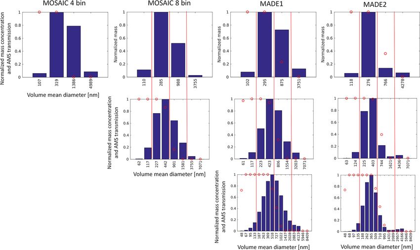
P. E. Saide et al.: Understanding and improving model representation of aerosol optical properties                                      6461

Table 3. Lower and upper diameters (µm) for the 4, 8, and 16 size bin configurations.

                            4-bin    Lower     Upper     8-bin    Lower       Upper    16-bin   Lower      Upper
                            Bin 1     0.039     0.156    Bin 1     0.039      0.078    Bin 1     0.039    0.0552
                            Bin 2     0.156     0.625    Bin 2     0.078      0.156    Bin 2    0.0552     0.078
                            Bin 3     0.625       2.5    Bin 3     0.156      0.312    Bin 3     0.078       0.11
                            Bin 4       2.5        10    Bin 4     0.312      0.625    Bin 4      0.11     0.156
                                                         Bin 5     0.625       1.25    Bin 5     0.156     0.221
                                                         Bin 6      1.25        2.5    Bin 6     0.221     0.312
                                                         Bin 7        2.5         5    Bin 7     0.312     0.442
                                                         Bin 8          5        10    Bin 8     0.442     0.625
                                                                                       Bin 9     0.625     0.884
                                                                                       Bin 10    0.884      1.25
                                                                                       Bin 11     1.25      1.77
                                                                                       Bin 12     1.77        2.5
                                                                                       Bin 13       2.5     3.54
                                                                                       Bin 14     3.54          5
                                                                                       Bin 15         5     7.07
                                                                                       Bin 16     7.07         10

Figure 4. (a) Time series of rubidium (grey, left axis, measured by the AMS), black carbon (black dashed line, right axis, measured by SP2),
and total organic aerosol (green, right axis, measured by AMS) during the haze event sampled by the NASA DC-8 over the Yellow Sea.
Rubidium was quantified using the AMS difference signal, a relative ionization efficiency of 1, and the same collection efficiency as the rest
of the submicron aerosol (Nault et al., 2018). (b) Average size-resolved AMS measurements sampled (aerodynamic diameter) by the NASA
DC-8 for the same period shown in (a).

saturation expected) the LAS measures larger volume con-                    these sources and would account for the minority of the mass
centrations than the AMS+SP2 by ∼ 11 %. Although 11 %                       for these emissions (Dillner et al., 2006). Also, the detection
falls within the stated accuracies of both measurements, it                 shown here is likely a lower limit of the actual concentra-
also potentially reflects a true difference in concentrations.              tions considering the refractory nature of aerosols typically
The AMS detected exotic metals not typically reported, such                 containing rubidium. The presence of rubidium would sug-
as rubidium (Fig. 4a), in the haze event. There was, on aver-               gest other inorganic material present in the haze event not
age, 10 ng sm−3 of rubidium in the plume between 01:30 and                  typically measured by the AMS, further suggesting that the
05:00 UTC (and up to 71 ng sm−3 ). Rubidium originates ei-                  11 % difference in volume is due to these types of com-
ther from soil (e.g., dust; Kabata-Pendias and Pendias, 2001)               pounds. Thus, we corrected the LAS submicron number and
or anthropogenic emissions, such as dust from steel and alu-                volume distributions using the aerosol mass measured by
minum industries (Dillner et al., 2006; Tang et al., 2018).                 the AMS+SP2 accounting for the ∼ 11 % volume not de-
Rubidium is one of numerous types of metal emitted from                     tected. For this, scaling factors were computed using the

https://doi.org/10.5194/acp-20-6455-2020                                                     Atmos. Chem. Phys., 20, 6455–6478, 2020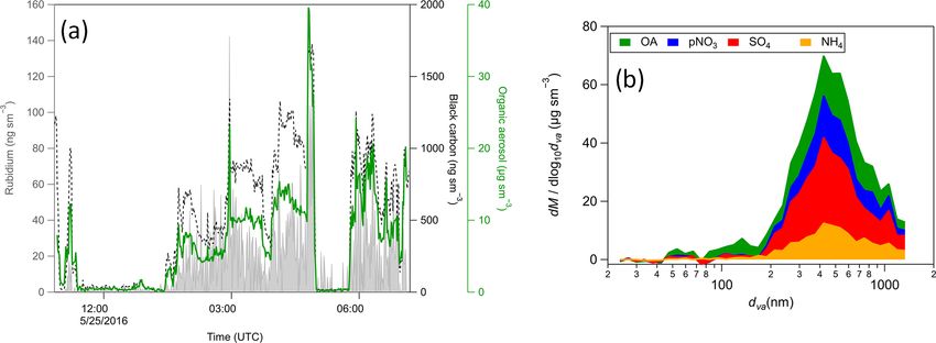
6462 P. E. Saide et al.: Understanding and improving model representation of aerosol optical properties
aerosol volume (estimated using the measured aerosol mass
and the aerosol density reported by the AMS), corrected by
11 %, and dividing by the measured LAS volume, account-
ing for the AMS transmission. The AMS transmission con-
siders 100 % and 0 % efficiency at aerodynamic diameters of
550 nm and 1.5 µm, respectively, and a linear decrease be-
tween using the logarithm of the aerodynamic diameters (Hu
et al., 2017). The transmission curve was converted to a ge-
ometric diameter for each observation using Eq. (28) from
DeCarlo et al. (2004) iteratively to update the Cunningham
slip correction factor until convergence. The LAS correction
assumes that the fractional contribution of aerosol not mea-
sured by AMS+SP2 is constant, which is a limitation of the
approach, but we expect it to have a limited impact on the
analysis due to the small contribution. The submicron dust
aerosol mass concentration is estimated using this volume
residual, assuming a dust density of 2.6 g cm−3 (value used
in WRF-Chem), and falls into the OIN aerosol category when
comparing to model estimates.
2.4 Ground-based observations
We also used multiple sources of ground-based observa-
tions. This includes Level 2.0 AOD at 500 nm wavelength,
which was obtained from the Aerosol Robotic Network
(AERONET; Holben et al., 1998) version 3 algorithm (Giles
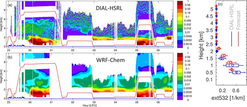
et al., 2019). During KORUS-AQ, the AERONET team en- Figure 5. Time series of box and whisker plots for AOD (a),
hanced the long-term AERONET sites with a short-term PM10 (b), and PM2.5 (c) for select days in the month of May 2016,
DRAGON network (Holben et al., 2018) to assess the comparing observations and forecasts over sites in South Korea.
mesoscale spatial variability of aerosol properties; thus, a to- Data are aggregated by day (in UTC). Center solid lines indicate
tal of 21 locations were available during the campaign pe- the median, circles represent the mean, boxes indicate upper and
riod. We also used PM2.5 and PM10 from the air quality net- lower quartiles, and whiskers show the upper and lower deciles.
work maintained by the Korean National Institute of Envi-
ronmental Research (NIER). For the period analyzed, PM2.5
and PM10 data were available from 320 and 329 locations, ary pollution coming from China (25 and 26 May), some-
respectively, distributed across the peninsula. times exceeding a factor of 2 difference. This points towards
model deficiencies in connecting surface mass concentra-
3 Results and discussion tions with column optical properties, which is explored in
this study focusing on the day the aircraft sampled this air
3.1 Forecast evaluation mass (24 May). Also note that PM2.5 and PM10 are similar
in the model, while PM10 is larger than PM2.5 in the obser-
Figure 5a shows comparisons of AOD measured by the vations (reflected in the differences in mean bias), pointing
AERONET network over South Korea versus forecasted towards model biases in representing coarse-mode aerosols.
AOD at the site locations. The model shows good perfor- Figure 6 shows observed and forecasted AOD retrievals
mance over the period (e.g., mean AOD for observations and at noon local time the day of the 24 May DC-8 flight that
the model is 0.58 and 0.60, respectively). This performance sampled the transboundary pollution that affected the Ko-
is expected as the system is assimilating satellite AOD, and rean Peninsula. The forecasts shown have not yet assimilated
satellite AOD retrievals have shown good agreement with the AOD retrieved that day, showing the ability of the sys-
AERONET data in the region (Choi et al., 2019b). However, tem to carry forward the information assimilated the day be-
the forecasts generally show large overpredictions of sur- fore. AODs larger than 1 were found over areas in the Yel-
face particulate matter for the period of large concentrations low Sea that were correctly forecasted and that enabled the
in the peninsula (mean bias for PM2.5 and PM10 is 44 and KORUS-AQ team to plan a successful flight (track in yellow
21 µg m−3 , respectively), consistent with previously reported in Fig. 6c) in the region. Data from this flight are used to
results (Lennartson et al., 2018). These overpredictions are perform a detailed model evaluation to understand the model
more severe for PM2.5 during the passing of the transbound- biases.
Atmos. Chem. Phys., 20, 6455–6478, 2020 https://doi.org/10.5194/acp-20-6455-2020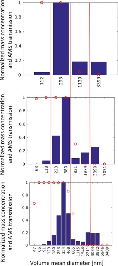
P. E. Saide et al.: Understanding and improving model representation of aerosol optical properties 6463
Figure 6. Observed (a) and forecasted (b) AOD maps at 03:00 UTC (noon local Korean time) on 25 May. (c) Advanced Himawari Imager true
color imagery for the same time with overlays of the DC-8 (in yellow) and Twin Otter (in red) flight tracks for that day (source: KORUS-AQ
flight report).
One potential reason for the discrepancies found could be 3.2 Closure studies
related to the model representation of aerosol vertical pro-
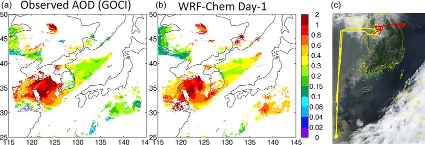
files. Figure 7 shows aerosol extinction curtains over the DC- Model representation of optical properties can be separated
8 trajectory (aircraft altitude in red solid line) as sampled by into two stages: (1) how well the model represents the
the DIAL-HSRL and as predicted by the forecasts. The haze aerosol properties that drive the optical properties compu-
layer is mostly confined to below 2 km, which the model rep- tation (e.g., size distribution, composition, concentrations,
resents properly (e.g., mean extinction in this layer for the etc.); and (2) the accuracy of the optical properties code. The
observations and model is 0.44 and 0.38 km−1 , respectively). latter can be evaluated by driving the optical properties code
The model has slightly higher mixing layers, which, if any- using observed quantities and comparing the outputs with
thing, would lead to opposite biases (e.g., underestimation of measurements of aerosol optical properties, a methodology
surface concentrations). A layer with lower aerosol extinc- that has been applied for previous field campaigns (Barnard
tion found between 2 and 6 km, which DIAL-HSRL classi- et al., 2010; Brock et al., 2016a) and that we will refer to as a
fied as dust (not shown) and where SAGA reported elevated “closure study” here. This allows us to isolate issues regard-
levels of Ca+2 associated with dust, is also well captured by ing the optical properties code and to assess ways to improve
the model in terms of both aerosol type and amount (mean the model representation of optical properties.
extinction in this layer during 00:00–01:00 UTC for the ob- One challenge of closure studies is that the optical proper-
servation and model is 0.012 and 0.015 km−1 respectively). ties code requires speciated and size-resolved aerosols; thus,
Thus, we discard issues with the model representation of the assumptions need to be made on how to distribute the mea-
vertical placement of the plume as reasons explaining the sured chemical species into the size bins. Figure 3a shows
AOD to PM inconsistencies mentioned earlier. a scatterplot of SAGA filter-based vs. AMS online measure-
AOD is also highly sensitive to relative humidity (Brock et ments of inorganic aerosol mass concentrations (sulfate, ni-
al., 2016a), and previous studies have explained AOD biases trate, ammonium, chloride), showing good agreement for this
due to model issues representing relative humidity (Feng et flight. While secondary inorganic aerosol mass concentra-
al., 2016). In situ measurements of relative humidity in the tions were elevated in the coarse mode for other KORUS-AQ
haze layer showed average values of 62 % with an interquar- flights (and thus not detected by AMS; Heim et al., 2020), for
tile range of 9 % (57 %–66 %). The forecast shows a rea- the flight analyzed here this fraction seems to be negligible.
sonable representation with a slightly higher average value Thus, we assume that the tail of the coarse mode is composed
(64 %) and interquartile range (10 %). Thus, we conclude that of only OINs (likely dust). We also assume that the compo-
skill in predicting relative humidity is not related to the dis- sition is not size-dependent within the accumulation mode.
crepancies found in this study. Size-resolved AMS measurements support this assumption
From this analysis, we conclude that the likely reason for by showing a similar composition within the accumulation
the discrepancy resides in the computation of the aerosol op- mode (Fig. 4b). We set the aerosol diameter cutoff between
tical properties, i.e., how aerosol mass is translated to AOD, the accumulation mode and the lower tail of the coarse mode
and thus in the following sections we perform a thorough at 884 nm based on size distribution measurements (Fig. 8).
evaluation of this topic using in situ airborne data. Also, since both LAS and APS cover the lower tail of the
coarse mode, we use APS estimates in this range because
LAS presents lower volume concentrations.
https://doi.org/10.5194/acp-20-6455-2020 Atmos. Chem. Phys., 20, 6455–6478, 2020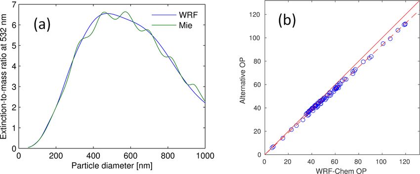
6464                    P. E. Saide et al.: Understanding and improving model representation of aerosol optical properties

Figure 7. DIAL-HSRL (a) and WRF-Chem forecast simulation (b) extinction curtains at 532 nm for the KORUS-AQ flight on 24 May.
The red solid line represents the altitude of the aircraft from which DIAL-HSRL was being operated. (c) Box and whisker plots as in
Fig. 5, aggregating the observed and modeled data shown in panels (a, b) for the periods during which the aircraft was above the haze layer
(00:00–01:00 and 05:00–05:45 UTC).

Table 4. Description of closure cases. Refer to Sect. 3.2 for defini-   between dry extinction and the aerosol volume concentration
tions of the base and updated configurations. Size bins are defined     obtained from the aerosol size distribution measurements
in Table 3.                                                             after performing the corrections described in Sect. 2.3. As
                                                                        AMS and SP2 measure mostly submicron aerosols of select
  Name         No. of size    Refractive index    Hygroscopicity        chemical species, there is potential for unaccounted aerosol
                      bins
                                                                        mass contributing to aerosol extinction that could complicate
  Closure 1              4    Base                Base                  the interpretation of the mass extinction efficiency. There-
  Closure 2              8    Base                Base                  fore, the volume extinction efficiency is reported in addition
  Closure 3             16    Base                Base                  to the mass extinction efficiency as the extinction and volume
  Closure 4             16    Updated             Base                  are measured for all aerosols in the same size range (behind
  Closure 5             16    Updated             Updated               the LARGE inlet).
                                                                           Figure 9a and b clearly show how the base configuration
                                                                        of the optical properties code drastically underpredicts the
   Figure 9 shows multiple statistical metrics in the form of           mass and volume extinction efficiencies (e.g., mean mass ex-
box and whisker plots for observations and closure results              tinction efficiency for the observations and Closure 1 is 6.7
during the three consecutive hours that the DC-8 spent mea-             and 4.5 m2 g−1 , respectively), consistent with the discrepan-
suring the haze layer at multiple altitudes (02:00–05:00 UTC;           cies shown in Fig. 5. Aerosols are binned into four size bins
see Fig. 7). The different closure scenarios are described in           in the base configuration (Closure 1); thus, Closures 2 and
Table 4 and consist of the base configuration and then the              3 explore finer binning to 8 and 16 sections, respectively.
base with varying parameters such as the size bin resolution,           The finer binning does improve the performance, especially
refractive indices, and hygroscopicity parameter.                       when going from four to eight bins (average mass extinc-
                                                                        tion efficiencies of 4.5 and 5.0 m2 g−1 , respectively). Figure 8
3.2.1   Dry extinction                                                  shows the size distributions for the three types of size aggre-
                                                                        gation, showing a large diversity in the bin concentrations
A variable that is typically computed to assess the efficiency
                                                                        contributing to the total mass in fine-resolution bins, which
of an aerosol population at scattering light is the ratio be-
                                                                        is lost when aggregating to coarser-resolution bins. Figure 10
tween dry extinction (scattering) and aerosol mass concentra-
                                                                        shows steep changes in the volume extinction efficiency for
tions, which is typically referred to as “mass extinction (scat-
                                                                        the diameters at which most of the aerosol mass is found
tering) efficiency”. Note that for this study, the aerosol mass
                                                                        (200–500 nm). In the four-bin configuration, the whole ac-
concentration corresponds to that measured by AMS+SP2.
                                                                        cumulation mode is included in one bin. After aggregation,
We also define “volume extinction efficiency” as the ratio

Atmos. Chem. Phys., 20, 6455–6478, 2020                                                    https://doi.org/10.5194/acp-20-6455-2020
P. E. Saide et al.: Understanding and improving model representation of aerosol optical properties 6465
Figure 8. Resulting average size distributions (blue bars) when ag-
gregating observed data (02:00–05:00 UTC) to 4, 8, and 16 size
bins. Sizes distributions show the average mass concentration in
each bin normalized by the maximum value within each distribu-
tion. Red lines separate bins aggregated when going from a finer to
coarser bin representation. Size bins boundaries are defined in Ta-
ble 3. Red circles indicate the average AMS transmission efficiency
Figure 9. Box and whisker plots (as in Fig. 5) showing observa-
(dimensionless) for each size bin.
tions and closure results driving the optical properties code with
observations. Closure cases are described in Table 4. Results are
shown for (a) the extinction-to-mass ratio (550 nm; mass extinction
efficiency), (b) extinction-to-volume ratio (volume extinction effi-
ciency), (c) f (RH) measured at 550 nm, (d) the 550–700 Ångström
a mean diameter of 293 nm is obtained, which has a volume exponent, and (e) dry single-scattering albedo. The blue numbers
extinction efficiency below 6 m2 m−3 with base refractive in- on top of the plots represent the sample size used when computing
dices. On the other hand, a large percentage of the accumu- statistics.
lation mode is found in bin no. 4 with the eight-bin configu-
ration, which has a mean diameter of 380 nm and a volume
extinction efficiency of ∼ 8 m2 m−3 ; this raises the overall base refractive indices. Negligible improvements are found
efficiency substantially. The improvements from 8 to 16 bins when further refining from 16 to 32 size bins (not shown).
are lower than from four to eight bins, but they are still signif- Although improvements are found when refining the size
icant and due to similar reasons. For instance, bin no. 8 in the bins, significant biases still persist for the 16-bin configu-
16-bin configuration shows a volume extinction efficiency ration (Fig. 9a, b). Thus, we explore modifying the refrac-
above 9 m2 m−3 , getting close to the maximum values for tive indices used in the Mie calculation (see Sect. 2.3) based
https://doi.org/10.5194/acp-20-6455-2020 Atmos. Chem. Phys., 20, 6455–6478, 20206466 P. E. Saide et al.: Understanding and improving model representation of aerosol optical properties Figure 10. (a) Volume extinction efficiency (blue, scale on the left) and f (RH) (orange, scale on the right) as a function of geometric dry particle diameter considering a monodisperse aerosol distribution of fixed aerosol composition equal to the mean of the data analyzed. Different lines represent cases in which the real refractive index and hygroscopicity correspond to the base and updated conditions (see text for details). Black markers on top of the plots represent the calculated volume mean diameter for each size bin when using 4 (circles), 8 (squares), and 16 (x) bins for the mean observed size distribution (numerical values found in Fig. 8). Note that only mean diameters below 1 µm are shown. (b) Same as (a) but for dry single-scattering albedo and the 550–700 nm Ångström exponent. on values reported in the literature for the aerosol species efficiencies vs. particle dry diameter achieves its maximum accounting for the most submicron mass. Typical real re- (Fig. 10a). The update in the OA refractive index generates fractive indices assumed in closure studies (e.g., Brock et the most impact (not shown) due to the larger increase (7 % al., 2016a) for ammonium sulfate and ammonium nitrate change vs. 0.5 % and 3.5 % for ammonium sulfate and am- are 1.527 (Hand and Kreidenweis, 2002) and 1.553 (Tang, monium nitrate, respectively) and large contribution to the 1996), which are larger than those used in the base config- total mass (23 % on average). uration, and thus we update them accordingly. For primary and secondary organic aerosols, there is a large range of val- 3.2.2 Hygroscopic growth ues found in the literature (e.g., Moise et al., 2015; Lu et al., 2015). Aldhaif et al. (2018) derived the organic aerosol (OA) While the analysis in the previous subsection was performed real refractive index from field deployments by air mass type, for dry aerosol extinction, we also explored possible biases finding a mean value of 1.54 with 1.52–1.55 as the 25–75th due to hygroscopic growth, considering that relative humid- percentile range for urban air masses. We chose the value of ity was in the 50 %–80 % range in the haze layer. We assessed 1.55 as it is in the 25–75th percentile range and because it is the performance of the optical properties code, driven by ob- a typical value used in past studies (Zhang et al., 1994; Hand served inputs in representing the aerosol light-scattering en- and Kreidenweis, 2002; Hodzic et al., 2004). This value also hancement factor (f (RH)), defined here as the ratio between corresponds to the mean real refractive index reported by Lu 550 nm aerosol scattering at 80 % (wet) and 20 % (dry) rela- et al. (2015) for primary organic aerosol based on a literature tive humidity. review. The Closure 4 case includes these updates (summary Figure 9c shows that the base configuration performs well of updated parameters in Table 2), showing an increase in the for f (RH) (average of 2.2 vs. 2.1 for observations and Clo- efficiencies that improves the model representation (Fig. 9a, sure 1, respectively). This is due to a combination of the b). Although the mass and volume extinction efficiencies are wrong reasons (i.e., cancellation of errors), as it deteriorates still underpredicted (e.g., average mass extinction efficien- when increasing the size bin resolution (Closures 2 and 3) cies of 6.7 and 6.1 m2 g−1 for observations and Closure 4, and upon increasing the refractive indices (Closure 4), go- respectively), there is much better agreement when using the ing down to average values as low as 1.7. Figure 10a ad- updated refractive indices, obtaining an overlap of the ob- ditionally shows f (RH) and can help explain this behavior, served and modeled 25–75th percentile boxes. Besides the as f (RH) has a strong decreasing trend with increasing di- overall increase in the efficiencies, there is also a slight shift ameter in the region < 350 nm. Thus, because the four-bin towards smaller sizes for the location where the curve of representation displays an apparent decrease in the mean di- Atmos. Chem. Phys., 20, 6455–6478, 2020 https://doi.org/10.5194/acp-20-6455-2020
P. E. Saide et al.: Understanding and improving model representation of aerosol optical properties                         6467

ameter (Fig. 7), f (RH) is overestimated. As the size bins        tation of both AE and SSA improves when going from the
are refined, less aerosol mass falls in the smaller size bins,    coarse size bin resolution and base parameters to the finer
decreasing the total f (RH). The further decrease in f (RH)       bin and updated parameters, which represents independent
with increasing refractive indices at these size ranges is also   pieces of evidence that the change in configuration is in the
shown in Fig. 10a. While our alternative approach at comput-      right direction. As seen in Fig. 10b, AE is sensitive to the
ing aerosol water uptake resulted in values ∼ 7 % lower than      aerosol size distribution and generally decreases with larger
that shown by WRF-Chem, the difference in the observed vs.        aerosol sizes. This explains the sharp decrease when refin-
Closure 4 f (RH) are close to 30 %; thus, we conclude that        ing the aerosol size bins (mean AE drops from 2.4 in Clo-
similar biases would be expected for the WRF-Chem rou-            sure 1 to 2.2 in Closure 2) due to the lower mean diameters
tines.                                                            for the four-bin configuration as described previously. Fig-
   To improve the optical properties code performance, we         ure 9e shows that SSA gradually increases with the change
updated the hygroscopicity parameter based on values found        in configuration (from 0.92 in Closure 1 to 0.94 in Closure 5),
in the literature for the species contributing to most of the     which is due to changes in mean diameters and higher scat-
aerosol mass. κ values are generally reported with a large        tering when increasing the real refractive indices (Fig. 10b).
range of uncertainty and can depend on the measurement            While the AE of Closure 5 matches the observed values very
technique and environmental conditions. Petters and Krei-         well (mostly due to improvements from Closure 1 to 2), SSA
denweis (2007) show a wide range of κ values for ammo-            is still slightly underpredicted (mean observation of 0.95),
nium sulfate (from 0.33 to 0.72 with a mean of 0.53) and          which is an issue previously identified in other closure stud-
for κ derived using growth factors, with a mean value of          ies using a similar approach for computing aerosol optical
0.61 based on cloud condensation nuclei (CCN) measure-            properties (Barnard et al., 2010). This underestimation could
ments. For ammonium nitrate, only CCN-derived κ is avail-         be due to multiple uncertainties including assumptions on
able, with a mean value of 0.67 and a range of 0.577–0.753.       black carbon and OIN complex refractive indices, black car-
We chose to use the mean values of the CCN-derived esti-          bon mixing state, and the size-independent black carbon frac-
mates (0.61 for ammonium sulfate and 0.67 for ammonium            tional contribution to the accumulation mode.
nitrate), as they are contained in the ranges provided in Pet-
ters and Kreidenweis (2007) and in other studies (e.g., Good      3.3   Evaluation of retrospective simulations
et al., 2010). For organic aerosol, the range is even larger.
We chose to treat organic aerosol and OINs as slightly hy-        The previous section provides clarity on what we should
groscopic, as was originally specified in the WRF-Chem pa-        expect from the optical properties code if the model is re-
rameterization for GOCART, with κ values of 0.14 for both,        producing observed aerosol size distributions and composi-
which is consistent with values reported for aged urban OA        tion. In this section we perform a similar analysis but driving
and for rural environments (Wang et al., 2010; Mei et al.,        the optical properties code with simulated aerosol properties
2013; Levin et al., 2014). κ of sodium chloride was updated       (summarized in Table 1 and shown in Fig. 11). Comparing
to 1.1 following the revisions of Zieger et al. (2017) to con-    Fig. 11a and b, we can see large discrepancies in the per-
sider the properties of inorganic sea salt. This large decrease   formance of the mass and volume extinction efficiencies that
in κ has little impact for the study period as sea salt mass      are opposite to the closure studies (Fig. 9) for which they
concentrations represented less than 1 % of the total in both     remain consistent. For instance, MOSAIC4b shows a good
observations and models. A summary of the updated κ val-          representation for the mass extinction efficiency against Clo-
ues can be found on Table 2. Figure 9c shows significant          sure 5 (mean of 6.4 and 6.2 m2 g−1 , respectively) but largely
increases in f (RH) from Closure 4 to Closure 5 (average          underestimates the volume extinction efficiency (mean of 4.5
f (RH) of 2.1) up to a similar level as the observations. Sen-    and 7.5 m2 m−3 , respectively). Comparing Figs. 11 and 9,
sitivity analysis shows that most of the change is related to     the mass extinction efficiency is shifted up in the three base
the κ increases in ammonium sulfate and ammonium nitrate          modeling configurations, and thus a refinement in size bins
due to their larger contribution to the mass fraction (62 % on    (going from MOSAIC4bin to MOSAIC8b or MADE1) has
average), while additional water uptake of organics and other     the opposite effect on performance for mass and volume ex-
inorganic aerosols play a minor role. Thus, choosing a lower      tinction efficiencies. The modeled aerosol mass concentra-
OA κ value more consistent with other studies (Brock et al.,      tion used when computing the mass extinction efficiency is
2016a; Shingler et al., 2016) would have resulted in similar      that for which the AMS transmission is applied. Thus, one
findings.                                                         possible explanation could be that the models have signifi-
                                                                  cant aerosol mass outside the sizes the AMS can detect. This
3.2.3   Other aerosol optical properties                          would reduce the mass concentration after applying the trans-
                                                                  mission curve, which would increase the extinction-to-mass
Figure 9d and e show the change for the Ångström expo-            ratio (i.e., the mass extinction efficiency) due to the unac-
nent (AE) and single-scattering albedo (SSA) for the dif-         counted mass that contributes to extinction. Figure 12 shows
ferent model closure configurations. Overall, the represen-       the size distributions and AMS transmission efficiency for

https://doi.org/10.5194/acp-20-6455-2020                                           Atmos. Chem. Phys., 20, 6455–6478, 2020
You can also read