Simulating shrubs and their energy and carbon dioxide fluxes in Canada's Low Arctic with the Canadian Land Surface Scheme Including Biogeochemical ...
←
→
Page content transcription
If your browser does not render page correctly, please read the page content below
Biogeosciences, 18, 3263–3283, 2021
https://doi.org/10.5194/bg-18-3263-2021
© Author(s) 2021. This work is distributed under
the Creative Commons Attribution 4.0 License.

Simulating shrubs and their energy and carbon dioxide fluxes in
Canada’s Low Arctic with the Canadian Land Surface Scheme
Including Biogeochemical Cycles (CLASSIC)
Gesa Meyer1,2 , Elyn R. Humphreys2 , Joe R. Melton1 , Alex J. Cannon1 , and Peter M. Lafleur3
1 Environment  and Climate Change Canada, Climate Research Division, Victoria, BC, Canada
2 Geography  and Environmental Studies, Carleton University, Ottawa, ON, Canada
3 School of Environment, Trent University, Peterborough, ON, Canada

Correspondence: Gesa Meyer (gesa.meyer@canada.ca)

Received: 9 December 2020 – Discussion started: 29 December 2020
Revised: 9 April 2021 – Accepted: 18 April 2021 – Published: 2 June 2021

Abstract. Climate change in the Arctic is leading to shifts      The revised model, however, tends to overestimate gross pri-
in vegetation communities, permafrost degradation and al-        mary productivity, particularly in spring, and overestimated
teration of tundra surface–atmosphere energy and carbon (C)      late-winter CO2 emissions. On average, annual net ecosys-
fluxes, among other changes. However, year-round C and en-       tem CO2 exchange was positive for all simulations, suggest-
ergy flux measurements at high-latitude sites remain rare.       ing this site was a net CO2 source of 18 ± 4 g C m−2 yr−1
This poses a challenge for evaluating the impacts of climate     using shrub PFTs, 15 ± 6 g C m−2 yr−1 using grass PFTs,
change on Arctic tundra ecosystems and for developing and        and 25 ± 5 g C m−2 yr−1 using tree PFTs. These results high-
evaluating process-based models, which may be used to pre-       light the importance of using appropriate PFTs in process-
dict regional and global energy and C feedbacks to the cli-      based models to simulate current and future Arctic surface–
mate system. Our study used 14 years of seasonal eddy co-        atmosphere interactions.
variance (EC) measurements of carbon dioxide (CO2 ), water
and energy fluxes, and winter soil chamber CO2 flux mea-
surements at a dwarf-shrub tundra site underlain by continu-
ous permafrost in Canada’s Southern Arctic ecozone to eval-      Copyright statement. The works published in this journal are
uate the incorporation of shrub plant functional types (PFTs)    distributed under the Creative Commons Attribution 4.0 License.
                                                                 This license does not affect the Crown copyright work, which
in the Canadian Land Surface Scheme Including Biogeo-
                                                                 is re-usable under the Open Government Licence (OGL). The
chemical Cycles (CLASSIC), the land surface component of         Creative Commons Attribution 4.0 License and the OGL are
the Canadian Earth System Model. In addition to new PFTs,        interoperable and do not conflict with, reduce or limit each other.
a modification of the efficiency with which water evaporates
from the ground surface was applied. This modification ad-       © Crown copyright 2021
dressed a high ground evaporation bias that reduced model
performance when soils became very dry, limited heat flow
into the ground, and reduced plant productivity through wa-      1   Introduction
ter stress effects. Compared to the grass and tree PFTs previ-
ously used by CLASSIC to represent the vegetation in Arctic      The terrestrial carbon (C) cycle of the Arctic is changing as
permafrost-affected regions, simulations with the new shrub      the region warms at more than twice the rate of the rest of
PFTs better capture the physical and biogeochemical im-          the world (IPCC, 2014; Post et al., 2019). Enhanced Arctic
pact of shrubs on the magnitude and seasonality of energy        soil C loss to the atmosphere and waterways is linked to per-
and CO2 fluxes at the dwarf-shrub tundra evaluation site.        mafrost degradation and thermokarst processes, deeper ac-
                                                                 tive layers, deeper snow, and more frequent and intense fires

Published by Copernicus Publications on behalf of the European Geosciences Union.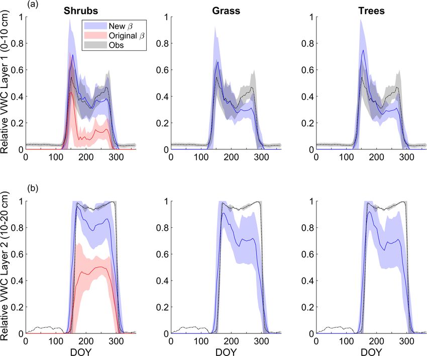
3264                                          G. Meyer et al.: Simulating high-latitude shrubs at a dwarf-shrub tundra site

(Hayes et al., 2014; Abbott et al., 2016; Myers-Smith et al.,      to project C flux trends into the future (McGuire et al., 2018;
2019, 2020; Belshe et al., 2013b; Turetsky et al., 2020). A        Post et al., 2019). Model estimates of C budgets are espe-
significant positive climate feedback effect is possible if even   cially important in the Arctic, as year-round flux measure-
a small proportion of the approximately 1035 ± 150 Pg C            ments are difficult to obtain and hence remain rare.
stored in the top 3 m of Arctic soils (Hugelius et al., 2014) is      It is critical that land surface models are able to capture
transferred to the atmosphere (Chapin et al., 2005; Schuur         the important interactions between the Arctic tundra and the
et al., 2009; Hayes et al., 2014). However, longer grow-           atmosphere due to potential feedbacks on regional and global
ing seasons and Arctic “greening” associated, in part, with        climate. The Canadian Land Surface Scheme Including Bio-
northward migration of the tree line and shrub expansion are       geochemical Cycles (CLASSIC, the open-source community
linked to increased growing season carbon dioxide (CO2 ) up-       model successor to CLASS-CTEM; Melton et al., 2020) rep-
take (Belshe et al., 2013a; Abbott et al., 2016; Myers-Smith       resents the land surface exchanges of energy, water, and C in
et al., 2011).                                                     the Canadian Earth System Model (CanESM) (Swart et al.,
   There are large uncertainties as to whether the Arctic tun-     2019) and has been extensively evaluated on a global scale
dra is currently an annual source or sink of CO2 (McGuire          (e.g., Melton and Arora, 2016; Arora et al., 2018). CLAS-
et al., 2012). Recent studies have highlighted the importance      SIC already focuses on several physical processes relevant
of CO2 emissions during the long winter and shoulder sea-          to the high latitudes, including treatment of snow and soil
son periods, which may offset CO2 gains by Arctic ecosys-          freeze–thaw processes (Melton et al., 2019) and peatland C
tems during the short growing season (Belshe et al., 2013a;        cycling (Wu et al., 2016). However, CLASSIC does not have
Oechel et al., 2014; Euskirchen et al., 2017; Arndt et al.,        a plant functional type (PFT) specific to tundra. Instead tun-
2020). Long-term trends in winter CO2 fluxes are generally         dra vegetation is represented by C3 grass and/or trees de-
difficult to ascertain due to a scarcity of year-round measure-    pending on land cover mapping. In reality, Arctic vegetation
ments, but several studies have suggested winter CO2 emis-         is diverse, consisting of erect or prostrate, evergreen or de-
sions are changing. Belshe et al. (2013a) found a significant      ciduous shrubs, graminoids, herbs, moss, and lichen (Chapin
increase in winter CO2 emissions over the 2004–2010 time           and Shaver, 1985). Although there are challenges in inter-
period using observations from six pan-Arctic sites. Natali        preting satellite-based trends of Arctic greening or browning
et al. (2019) up-scaled in situ measurements from about 100        (Myers-Smith et al., 2020), observed increases in greenness
high-latitude sites using a boosted regression tree machine        or productivity have been linked to shrub expansion through
learning model to estimate a contemporary loss of 1662 Tg C        infilling of patches, advances in shrubline, and increased
per year from the Arctic and boreal northern permafrost re-        height and abundance of shrub species (Myers-Smith et al.,
gion (land area ≥ 49◦ N) from October to April (2003–2017).        2011; Lantz et al., 2012). These kinds of changes in tun-
This winter loss of CO2 exceeded the average growing sea-          dra vegetation communities can affect snow and active-layer
son CO2 uptake estimated using five process-based mod-             depths, hydrology, surface–atmosphere energy exchange, nu-
els by over 600 Tg C per year. In addition to belowground          trient dynamics, and the terrestrial C balance of the Arctic
microbial respiration during the winter months, diffusion of       tundra (Myers-Smith et al., 2011).
stored CO2 produced during the non-winter period could                In order to further improve the representation of Arctic
have contributed, to an unknown extent, to the observed win-       surface–atmosphere interactions in CLASSIC, we evaluate
ter CO2 emissions (Natali et al., 2019). Using hourly at-          new dwarf deciduous and evergreen shrubs and sedge PFT
mospheric CO2 measurements, early-winter respiration rates         parameterizations with eddy covariance (EC)-based observa-
from Alaska’s North Slope tundra region are estimated to           tions of CO2 and energy fluxes at an erect dwarf-shrub tundra
have increased by 73 ± 11 % since 1975 (Commane et al.,            site in Canada’s Southern Arctic. We also address an evapo-
2017). However, both growing season and winter CO2 fluxes          ration (E) bias discovered in CLASSIC, which has important
from Alaska’s North Slope were not well represented by the         implications for appropriately simulating energy flux feed-
majority of 11 Earth system models (ESMs) from the Cou-            backs and water-stress impacts on growing season photosyn-
pled Model Intercomparison Project Phase 5 (CMIP5) inves-          thesis. For example, Sun and Verseghy (2019) found that soil
tigated by Commane et al. (2017). Most models predicted the        E was overestimated for mid-latitude shrublands during wet
start of the growing season earlier than observed, underesti-      periods in spring, which led to underestimation of evapotran-
mated early-winter CO2 losses, and overestimated annual net        spiration (ET) and photosynthesis in the summer. We com-
CO2 uptake (Commane et al., 2017).                                 pare our offline model simulations with C3 grass and tree pa-
   Field observations and process-based models are comple-         rameterizations to highlight how shrubs uniquely affect CO2
mentary approaches to better understand Arctic CO2 sink and        and energy exchange with the atmosphere. Finally, we use
source dynamics. Field observations may be used to parame-         CLASSIC to simulate winter CO2 fluxes and estimate the an-
terize and evaluate process-based models (Zhang et al., 2014;      nual CO2 budget for this tundra site, where winter flux mea-
Commane et al., 2017; Park et al., 2018; Huntzinger et al.,        surements are challenging to obtain.
2020), which are then applied over larger regions (McGuire
et al., 2012; Jeong et al., 2018; Ciais et al., 2019) and used

Biogeosciences, 18, 3263–3283, 2021                                                  https://doi.org/10.5194/bg-18-3263-2021
G. Meyer et al.: Simulating high-latitude shrubs at a dwarf-shrub tundra site                                                  3265

2     Methods                                                        face – e.g., Rn , soil temperatures, and water content (liquid
                                                                     and frozen) – from the physics sub-module.
2.1     CLASSIC
                                                                     2.1.2   Model modifications
2.1.1    Model description
                                                                     CLASSIC v1.0.1 uses four broad categories of PFTs (needle-
A detailed description of CLASSIC v1.0 can be found                  leaf trees, broadleaf trees, crops, and grasses) in its calcula-
in Melton et al. (2020). It couples a land surface                   tion of physical land surface processes (relating to energy,
physics sub-module (the Canadian Land Surface Scheme:                momentum, and water) in the physics sub-module. These are
CLASS; Verseghy, 2017) to a biogeochemistry sub-module               expanded to nine PFTs for simulating biogeochemical pro-
(the Canadian Terrestrial Ecosystem Model: CTEM; Melton              cesses, to account for different deciduous or evergreen plant
and Arora, 2016) as an open-source community successor               characteristics or for plants with C3 versus C4 photosynthetic
to CLASS-CTEM. Physical processes determining energy                 pathways.
and water balances of the land surface are implemented                  In this study, we added one more broad category PFT
in CLASS, described in detail in Verseghy (1991, 2000)               to the physics sub-module (shrubs) and three more PFTs
and Verseghy et al. (1993), and biogeochemical processes             to the biogeochemistry sub-module (cold broadleaf decid-
are handled by CTEM, described in detail in Arora (2003)             uous shrubs, broadleaf evergreen shrubs, and sedges), as
and Melton and Arora (2016).                                         these PFTs represent the broad categories of vascular veg-
   The atmospheric forcing variables required by CLAS-               etation most commonly found in Arctic tundra (e.g., Walker
SIC are incoming shortwave (RSW ) and longwave radiation             et al., 2005) or the understory of other northern high-latitude
(RLW ), air temperature (Ta ), the precipitation rate, air pres-     ecosystems such as the boreal forest. The biogeochemistry
sure (PA), specific humidity (q), and wind speed (U ). Driven        PFTs map onto the physics PFTs as shown in Table 1. Sedges
by these meteorological data, the transfer of heat and water         are considered a grass by the physics sub-module, while ev-
through the soil layers and snow, as well as the exchange            ergreen and cold deciduous shrubs are assigned to the shrub
with the atmosphere and within the vegetation canopy, is             PFT. The parameterizations developed by Wu et al. (2016)
typically calculated on a half-hourly time step when run of-         for the two shrub PFTs and a sedge PFT for a peatland-
fline. Net radiation (Rn ) is calculated using prognostically        specific sub-module for CLASS-CTEM were used as a start-
determined ground and snow albedo, the land surface tem-             ing point. Note that the peatland sub-module PFTs of Wu
perature, RSW , and RLW . CLASSIC enforces energy balance            et al. (2016) only considered the biogeochemical impacts of
closure. In previous versions of CLASS, soil layers were lim-        these PFTs. We fully integrate these new PFTs in order to
ited to three layers with a maximum soil depth of 4.1 m, but         simulate the physical impact of the shrub’s unique growth
CLASSIC allows for an arbitrary number of ground layers              form and function.
and deeper depths. In this analysis, we used 22 layers start-           The original CLASSIC formulation of ground E tended
ing with a thickness of 10 cm, which increased with depth,           to overestimate E during periods of water ponding on the
down to a depth of 20 m (Supplement, Table S1) following             ground surface or when the water content of the top soil
the recommendations by Melton et al. (2019) for permafrost-          layer, θ1 (m3 m−3 ), was high, e.g., during and after snowmelt
affected soils. Water movement between the soil layers oc-           (see Sect. 3.3 and Fig. 4c). This excessive E dried the soil
curs until the bottom of the permeable layer (set to 5 m in this     to such an extent that summer ET and gross primary pro-
study), while heat transfer is taken into account within the         ductivity (GPP) were underestimated due to water stress.
whole ground column, thus including the permeable layers             This issue was also observed at shrubland sites by Sun and
and the bedrock below. Energy, momentum, and water fluxes            Verseghy (2019), who reduced soil E by applying a site- or
are calculated on a 30 min time step including photosynthe-          soil-texture-specific scaling factor to the maximum surface
sis and canopy conductance. These fluxes are influenced by           evaporation rate (E(0)max ). For a more broadly applicable
vegetation characteristics such as vegetation height, leaf area      formulation, we adopted the approach of Merlin et al. (2011),
index (LAI), leaf and stem biomass, and rooting depth. These         which modifies the parameterization of the evaporation effi-
vegetation characteristics depend on PFT parameterizations           ciency coefficient (β). In CLASSIC, the potential evapora-
and are dynamically determined within the biogeochemistry            tion rate from bare soil, E (0) (mm s−1 ), is calculated as
sub-module through the allocation of C on a daily time step,         E(0) = ρa CDH Va (q(0) − qa ),                              (1)
which use the accumulated photosynthetic fluxes calculated
on the physics time step. In addition to C allocation to leaves,     where ρa is the air density (kg m−3 ), CDH is the surface drag
stems, and roots, the biogeochemistry sub-module simulates           coefficient for evaporation (unitless), Va is the wind speed at
other biogeochemical processes such as autotrophic (Ra ) and         reference height (m s−1 ), q (0) is the specific humidity at the
heterotrophic respiration (Rh ) from its leaf, stem, root, litter,   surface (kg kg−1 ), and qa is the specific humidity at the ref-
and soil C pools on a daily time step. The biogeochemistry           erence height (kg kg−1 ) (Verseghy, 2017). The surface evap-
sub-module obtains required information about the land sur-          oration rate is capped by a maximum value, E(0)max , deter-

https://doi.org/10.5194/bg-18-3263-2021                                                     Biogeosciences, 18, 3263–3283, 2021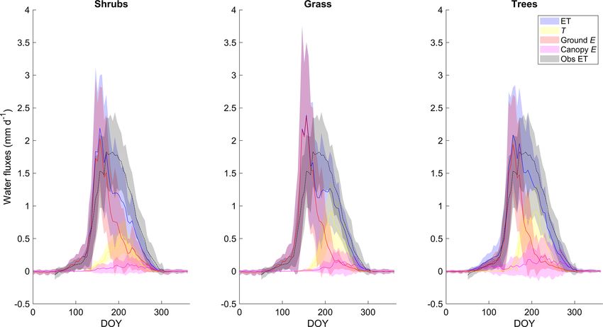
3266 G. Meyer et al.: Simulating high-latitude shrubs at a dwarf-shrub tundra site
Table 1. Mapping between plant functional types (PFTs) used in CLASSIC’s physics and biogeochemical calculations. PFTs in bold font
indicate the new PFTs incorporated by our study.
PFTs used in model PFTs used in model biogeochemical calculations
physics calculations
Needleleaf tree Evergreen Deciduous
Broadleaf tree Evergreen Cold deciduous Drought/dry deciduous
Crop C3 crop C4 crop
Grass C3 grass C4 grass Sedge
Broadleaf shrub Evergreen Deciduous
mined by θ1 and the depth of water ponded on the surface for shrubs as it was previously included for deciduous tree
(Zp , m) as species in CLASSIC. Following Bauerle et al. (2012) and Al-
ton (2017), seasonality was included by modifying Vcmax
E(0)max = ρw (Zp + (θ1 − θmin )1Z1 )/1t, (2) such that
with the water density ρw (kg m−3 ); the residual soil liquid
dayl 2
water content remaining after freezing or evaporation θmin Vcmax,new = Vcmax , (6)
daylmax
(m3 m−3 ), which is set to 0.04 m3 m−3 for mineral and fib-
ric organic soils; the depth of the top soil layer 1Z1 (e.g., with the current (dayl, hours) and annual maximum day
0.10 m); and the time interval 1t (s) (Verseghy, 2017). length (daylmax , hours) determined from the site’s latitude.
The saturated surface specific humidity (q(0)sat ), qa , and β Vcmax affects the maximum catalytic capacity of Rubisco
determine q (0) as (Vm , mol CO2 m−2 s−1 ; Melton and Arora, 2016).
Vegetation height, h (m), depends on stem biomass (Cs ;
q(0) = βq(0)sat + (1 − β)qa , (3) kg C m−2 ) in CLASSIC. Shrub h is calculated following Wu
et al. (2016) as h = min(0.25Cs0.2 , 4.0), but here we now al-
where β is defined using a relation by Lee and Pielke (1992)
low for taller shrubs with a maximum height of 4 m instead
as
of 1 m. Like grass, but unlike trees, shrubs can be buried by
0
for θ1 < θmin snow in CLASSIC.
2
β = 0.25(1 − cos(π θ1 /θfc )) for θmin < θ1 ≤ θfc (4) Table 2 lists the parameters that were adapted for the new
shrub PFTs (see Supplement for equations), including the
1 for θ1 > θfc ,
leaf life span (τL , years); specific leaf area (SLA, m2 kg−1 C);
maximum vegetation age (Amax , years); and the parame-
where θfc is the field capacity of the top soil layer (m3 m−3 ).
ter ι, which determines the root profile and thus affects root-
Merlin et al. (2011) suggested using the volumetric water
ing depth (dR , m). The minimum root-to-shoot ratio (lrmin )
content at saturation as the maximum water content instead
for shrubs determines the allocation of C between roots and
of θfc based on the fact that the quasi-instantaneous process
aboveground biomass in stems and leaves and was obtained
of potential evaporation is physically reached at saturation.
from Qi et al. (2019).
Thus, the definition of β is modified to
In C allocation calculations, the C in stems (Cs , kg C m−2 ),
roots (CR , kg C m−2 ), and leaves (CL , kg C m−2 ) has to sat-
(
0 for θ1 < θmin
β= 2
(5) isfy the following relationship
0.25(1 − cos(π θ1 /θp )) for θmin < θ1 ≤ θp ,
Cs + CR = ηCLκ (7)
where θp is the porosity of the top soil layer (m3 m−3 ). There-
fore, Eq. (5) limits β to values below 1 except when soils are (Melton and Arora, 2016) while also meeting the lrmin con-
fully saturated, which differs from the previous parameteri- dition
zation (Eq. 4), where β remained 1 until θ was less than θfc . CR
To incorporate shrub and sedge PFTs, several more mod- ≥ lrmin . (8)
CS + CL
ifications were made to CLASSIC. As the photosynthetic
capacity of Arctic shrubs is seasonally variable and has If the root-to-shoot ratio falls below lrmin , C is preferentially
been shown to depend on day length and maximum inso- allocated to roots (Melton and Arora, 2016). The parame-
lation (Chapin and Shaver, 1985; Shaver and Kummerow, ters η and κ are PFT-specific (Table 2). The parameter val-
1992; Oberbauer et al., 2013), especially in the fall, a sea- ues for trees, crops, and grasses are based on Lüdeke et al.
sonal variation of the maximum carboxylation rate by the Ru- (1994), while η and κ for shrubs were estimated from values
bisco enzyme (Vcmax , mol CO2 m−2 s−1 ) was implemented of Cs , CR , and CL for shrub tundra (Nobrega and Grogan,
Biogeosciences, 18, 3263–3283, 2021 https://doi.org/10.5194/bg-18-3263-2021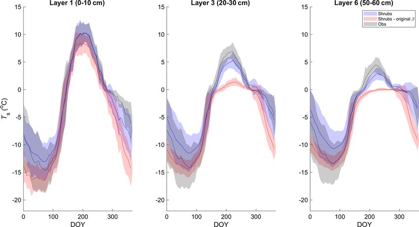
G. Meyer et al.: Simulating high-latitude shrubs at a dwarf-shrub tundra site                                                   3267

2007; Grogan and Chapin, 2000; Murphy et al., 2009; Wang           struments, Lymington, UK) operating at 10 Hz. The EC in-
et al., 2016), resulting in the same κ values as for grasses but   strumentation is mounted to a mast 4.1 m above the surface,
higher η (Table 2).                                                where 90 % of the total flux originates within 178 ± 21 m
                                                                   (± 1 standard deviation) from the flux tower determined us-
2.2     Model evaluation dataset                                   ing the flux footprint parameterization of Kljun et al. (2004).
                                                                   The tundra was well represented by the soil and vegetation
2.2.1    Study site                                                characteristics described above for at least 400 m in all direc-
                                                                   tions of the flux tower, and thus there was adequate fetch to
The study site at Daring Lake (AmeriFlux designation
                                                                   represent this tundra type. An open-path IRGA (model LI-
CA-DL1, hereafter referred to as DL1; 64◦ 52.1310 N,
                                                                   7500, LI-COR) was operated between 2004 and 2015, while
111◦ 34.4980 W) is located in Canada’s Northwest Territories,
                                                                   an enclosed-path sensor (LI-7200, LI-COR) has been oper-
approximately 300 km northeast of Yellowknife, at an ele-
                                                                   ated since 2014. The two IRGAs were run concurrently for
vation of 425 m. The climate is characterized by short sum-
                                                                   2014 and 2015 to develop a site-specific correction for the
mers and long, cold winters with a mean annual air temper-
                                                                   self-heating issue with the LI-7500 (Burba et al., 2008) de-
ature of −8.9 ◦ C (Lafleur and Humphreys, 2018) and 200 to
                                                                   scribed by Lafleur and Humphreys (2018). This correction
300 mm of precipitation on average (ECG, 2012). In better-
                                                                   was applied to all of the LI-7500 data. Half-hourly fluxes
drained areas, the surface soil organic layer is typically shal-
                                                                   are calculated using EddyPro™ (v. 6.2.0) (LI-COR) with
low, ranging from 1 to 10 cm in depth, deepening to 20 cm
                                                                   block averaging, a double coordinate rotation, and no an-
or more in wetter areas, with all areas underlain by coarse
                                                                   gle of attack correction. When the open-path IRGA oper-
textured mineral soil (sand to loamy sand) (Humphreys and
                                                                   ated, density fluctuations were addressed using the Webb
Lafleur, 2011). The average thaw depth in late summer is
                                                                   et al. (1980) approach; when the enclosed-path IRGA oper-
86 ± 3 cm (± SE) (Lafleur and Humphreys, 2018) measured
                                                                   ated, fluxes were computed directly from CO2 / H2 O mix-
over the period 2010–2015 using a metal probe inserted into
                                                                   ing ratios. The covariance of the vertical wind speed and
the soil at 40 points (10 points every 5 m in the four cardi-
                                                                   IRGA signals was used to compute time lags. Analytic cor-
nal directions around the measurement tower). DL1 is ap-
                                                                   rection of high- (Moncrieff et al., 2004) and low-pass (Mon-
proximately 70 km north of the treeline in Canada’s South-
                                                                   crieff et al., 1997) filtering effects was applied. Half-hourly
ern Arctic ecozone (ECG, 2012). The dominant vegetation at
                                                                   fluxes were removed from the time series due to sensor er-
DL1 includes evergreen shrubs (Rhododendron tomentosum,
                                                                   rors, due to power loss, or when associated variables (e.g.,
Empetrum nigrum, Loiseleuria procumbens) and deciduous
                                                                   vertical velocity, CO2 –H2 O concentrations) were outside ac-
shrubs (Betula glandulosa, Vaccinium uliginosum) (Lafleur
                                                                   ceptable ranges. A 0.1 m s−1 friction velocity threshold was
and Humphreys, 2018). Small variations in microtopography
                                                                   applied to CO2 fluxes at night and during snow-covered peri-
result in wet areas covering about 10 % of the area within
                                                                   ods (Lafleur and Humphreys, 2008). Half-hourly net ecosys-
200 m of the measurement tower, which support tussock-
                                                                   tem productivity (NEP) was calculated as the sum of the
forming sedges and Sphagnum species. Growing season vas-
                                                                   CO2 flux and the rate of change in CO2 storage below the
cular plant cover at DL1 was 63.6 ± 5.4 % determined us-
                                                                   4 m measurement height. The daily sum of turbulent energy
ing point frame measurements in July 2019 at 10 quadrats
                                                                   fluxes did not equal available energy most days (e.g., mean
with 25 points each. During the study period, the mean
                                                                   daily H  +LE
                                                                          Rn −G varied from 90 %–95 % mid-summer to 67 % on
LAI during July measured using a plant canopy analyzer
                                                                   average during the snow-melt period (Fig. S5 in the Supple-
(model LAI-2200, LI-COR Inc., Lincoln, NE, USA, (LI-
                                                                   ment); note that changes in energy storage between the EC
COR)) at 10 plots was 0.52 ± 0.05 (± SE) m2 m−2 , mean
                                                                   instrumentation and the ground surface were not included in
height of shrubs was 18.2 ± 1.3 cm (Lafleur and Humphreys,
                                                                   the evaluation of energy balance closure). LE and H were not
2018), and ground cover included mosses (percent ground
                                                                   adjusted for energy balance closure.
cover: 16.5 ± 4.9 %) and lichens (78.9 ± 5.0 %) (Lafleur and
                                                                      Half-hourly NEP was partitioned into GPP and ecosys-
Humphreys, 2018).
                                                                   tem respiration (Re ) using methods similar to those described
2.2.2    Measurements and data processing                          by Reichstein et al. (2005). An exponential temperature re-
                                                                   sponse function (Lloyd and Taylor, 1994) was parameterized
Eddy covariance flux measurements                                  using nighttime measurements of NEP (i.e., Re ) and Ta ,
                                                                                             1
Eddy covariance measurements of turbulent CO2 flux and en-                       E0 ( T          − 1 )
                                                                   Re = Rref e            ref −T0 Ta −T0   ,                      (9)
ergy fluxes and latent (LE) and sensible (H ) heat flux have
been made at DL1 during the growing season since 2004.             where Tref is set to 10 ◦ C and T0 is −46.02 ◦ C. Equation (9)
The measurements and data processing are described in de-          was first fit to the measurements within a moving window
tail by Lafleur and Humphreys (2018). Briefly, the EC system       period of 15 d moved in increments of 5 d. The average of all
consists of a CO2 –H2 O infrared gas analyzer (IRGA) and a         temperature sensitivity (E0 ) estimates which met the crite-
three-dimensional sonic anemometer (model R3-50, Gill In-          ria (between 0 and 450 K) was calculated (144.7 K) and ap-

https://doi.org/10.5194/bg-18-3263-2021                                                           Biogeosciences, 18, 3263–3283, 2021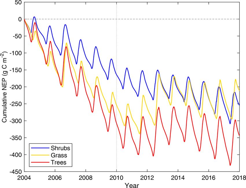
3268                                                        G. Meyer et al.: Simulating high-latitude shrubs at a dwarf-shrub tundra site

Table 2. CLASSIC’s biogeochemical parameter values for the PFTs used in this study, including the new PFTs (sedge, broadleaf evergreen
shrub, and broadleaf deciduous cold shrub). Equation numbers refer to those in this text or the Supplement. The parameters are Vcmax :
maximum carboxylation rate by the Rubisco enzyme; SLA: specific leaf area; τL : leaf life span; lrmin : minimum root-to-shoot ratio affecting
the allocation of C; ι: parameter determining the root profile and rooting depths; η and κ: parameters determining the minimum stem and
root biomass required to support the green leaf biomass; Amax : maximum vegetation age affecting the intrinsic mortality rate; ςD : litter base
respiration rate at 15 ◦ C; ςH : soil C base respiration rate at 15 ◦ C; χ : humification factor determining fraction of C transferred from the litter
to the soil C pool; ςS : stem base respiration rate at 15 ◦ C; ςR : root base respiration rate at 15 ◦ C; ςL : leaf maintenance respiration coefficient;
τS : turnover timescale for the stem; and τR : turnover timescale for the roots.

             Parameter        Eq.       Units                         Sedge       Broadleaf         Broadleaf           C3       Needleleaf        Needleleaf
                                                                                  evergreen        deciduous          grass       evergreen        deciduous
                                                                                      shrub        cold shrub                           tree             tree
             Vcmax            6         µmol CO2 m−2 s−1                  40               60               60           55                42                47
             SLA              S2        m2 kg−1                           10                8               15           –a                –a                –a
             τL               S1        Years                              1                2                1            1                 5                 1
             lrmin            8         Dimensionless                  0.30              1.68            1.68         0.50               0.16              0.16
             ι                S6        Dimensionless                  9.50              4.70            5.86         5.86               4.70              5.86
             η                7         Dimensionless                    3.0              6.0              6.0          3.0              10.0              30.8
             κ                7         Dimensionless                    1.2              1.2              1.2          1.2               1.6               1.6
             Amax             S3        Years                           n/ab             100              100          n/ab              250               400
             ςD               S10       kg C (kg C)−1 yr−1           0.5260           0.4453           0.5986       0.5260            0.4453            0.5986
             ςH               S10       kg C (kg C)−1 yr−1           0.0125           0.0125           0.0125       0.0125            0.0260            0.0260
             χ                S13       Dimensionless                  0.42              0.42            0.42         0.42               0.42              0.42
             ςS               S8        kg C (kg C)−1 yr−1               0.0           0.090            0.055           0.0            0.090             0.055
             ςR               S8        kg C (kg C)−1 yr−1            0.100            0.500            0.285        0.100             0.500             0.285
             ςL               S7        kg C (kg C)−1 yr−1            0.015            0.025            0.020        0.013             0.015             0.021
             τS               S12       Years                            0.0             65.0            75.0           0.0              86.3              86.3
             τR               S12       Years                            3.0             11.5            12.0           3.0              13.8              13.2
           a Determined by the model from the leaf life span. b In CLASSIC, A
                                                                             max is not defined for grasses and sedges, as the age-related mortality is not applied
           to these PFTs. n/a – not applicable.

plied to Eq. (9) to estimate the temperature-independent res-                              Eq. (9) was often poorly fitted during these periods. CO2 is
piration rate (Rref ) within consecutive 4 d periods. Finally,                             removed from the atmosphere and taken up by the ecosystem
the constant E0 and linearly interpolated Rref values were                                 when NEP and GPP values are positive. Positive Re indicate
used with Eq. (9) to calculate Re for all daytime half hours                               an emission of CO2 from the ecosystem to the atmosphere.
and nighttime half hours without measurements, as a means                                     Latent heat flux was gap-filled using daytime and night-
to gap-fill nighttime NEP. GPP was calculated as the sum                                   time regressions between LE and available energy for all
of NEP and Re . Missing daytime half-hourly estimates of                                   summer measurements. Estimates of LE were adjusted using
GPP were gap-filled by fitting a light response curve to all                               a multiplier to match observed LE within 4 d consecutive pe-
growing season GPP and photosynthetically active radiation                                 riods. Sensible heat flux was gap-filled as the difference be-
(PAR) (Eq. 10) and adjusting the resulting GPP estimates by                                tween available energy and gap-filled LE adjusted by a multi-
regressing these against previously estimated values within                                plier to account for changing energy budget imbalance. Daily
consecutive 4 d periods.                                                                   total CO2 and energy fluxes were calculated from gap-filled
                                                                                           traces only when there were at least 8 half hours of measured
          GPPmax αPAR
GPP =                  ,                                                       (10)        fluxes which passed all QA/QC criteria.
         αPAR + GPPmax
where GPPmax (µmol m−2 s−1 ) is the maximum                                                Forced diffusion chamber measurements
photosynthetic capacity at light saturation and α
(mol CO2 (mol PAR)−1 ) the quantum efficiency.                                             In order to measure soil CO2 efflux (assumed to represent
  Cold-season GPP was assumed to be negligible, and thus                                   Re ) during winter, three 10.1 cm diameter forced diffusion
NEP was equal to Re starting in the fall when the aver-                                    chambers (eosFD, Eosense Inc., Dartmouth, NS, Canada)
age Ta remained below −1 ◦ C for 3 consecutive days after                                  were installed ∼ 50 m NW of the DL1 flux tower in a sandy,
1 September of each year and until the snow had melted.                                    well-drained, and exposed area with little soil organic mat-
Cold-season NEP and Re were gap-filled using the average                                   ter. Measurements were available from 18 August 2018 to
cold-season observations during the 4 d window period as                                   19 May 2019. Implausible eosFD fluxes (21 % of the time se-

Biogeosciences, 18, 3263–3283, 2021                                                                                 https://doi.org/10.5194/bg-18-3263-2021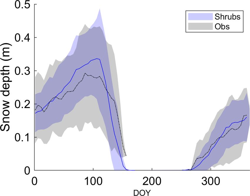
G. Meyer et al.: Simulating high-latitude shrubs at a dwarf-shrub tundra site                                              3269

ries) were excluded from analysis, including those indicating    water content (VWC) (water content reflectometer, CS615,
uptake of CO2 exceeding 0.5 µmol CO2 m−2 s−1 and those           CSI) at 7 and 20 cm depths (beginning in late August 2015
associated with atmospheric or internal concentrations below     for the 20 cm depth) in a drier area representative of the ma-
400 ppm, which suggested problems with the analyzer’s cal-       jority of the tower footprint; and G (soil heat flux plates at
ibration, the diffusion membrane, or other factors related to    7 cm depth, HFT3, CSI) adjusted to represent surface soil
gas transport through the frozen soil–snow–atmosphere sys-       heat flux using the rate of change in energy stored in the layer
tem. Daily total CO2 emissions were calculated from the av-      of soil above the plates. PAR reflectivity was calculated as the
erage of the remaining measurements.                             ratio of upwelling to downwelling PAR.
                                                                    Porosity, the liquid water content at wilting point, and
Meteorological measurements used to drive CLASSIC                other hydraulic and thermal soil properties are determined in
                                                                 CLASSIC using pedotransfer functions based upon the pre-
CLASSIC runs were forced using 30 min meteorological ob-         scribed soil textures (Cosby et al., 1984; Clapp and Horn-
servations at DL1 from 2004–2017. Measurements at DL1            berger, 1978). For organic soils, peat type (fibric, hemic, or
included the four Rn components downwelling and up-              sapric)-dependent values are assigned to θp and wilting point
welling shortwave and longwave radiation (CNR1, Kipp &           following Letts et al. (2000). The modelled porosity and
Zonen B.V., Delft, the Netherlands), PA (PTB101B Barome-         other soil properties did not necessarily correspond precisely
ter, Vaisala Oyj, Helsinki, Finland), Ta and relative humidity   to observed soil characteristics. For example, modelled θp for
(RH) at 1.5 m height (HMP-35C, Vaisala), U and wind di-          the surface organic layer and deeper mineral soil layers with
rection (propeller anemometer and wind vane at 1 m height;       80 % sand content was 0.93 and 0.39 m3 m−3 , respectively,
Wind Monitor, R.M. Young, Traverse City, MI, USA), rain-         while observed θp for the top 10 cm and deeper soil layers in
fall (tipping bucket rain gauge, TE525M, Texas Electronics,      the field was 0.77 and 0.46 m3 m−3 , respectively. Although
Dallas, TX, USA), and snow depth (sonic distance sensor,         there may be differences in the absolute VWC (m3 m−3 ),
SR50-L, CSI). Solid precipitation was estimated from in-         the pore water held in the soil between field capacity and
creases in snow depth over a 30 min time step using a sim-       wilting point matric potentials are likely comparable. To fa-
ple ratio of 1 mm water to 10 mm snow equivalent when Ta         cilitate this comparison, both observed and modelled VWC
was below −2 ◦ C. Specific humidity was calculated as q =        were scaled by their respective minimum and maximum val-
e·0.622             RH
 PA−e , where e = 100 ·es with the vapour pressure e (Pa) and    ues during 2004–2017 to produce a relative VWC value for
saturation vapour pressure es (Pa). Measurements of RSW ,        each time step following
RLW , PA, Ta , RH, U , and rainfall were gap-filled using du-
plicate sensors at nearby Daring Lake weather stations and       VWC(t) = (θ (t) − θmin )/(θp − θmin ).                     (11)
flux towers located within 2 km of the DL1 flux tower after      2.2.4   Bias-corrected reanalysis climate data
adjusting for offsets. Any remaining gaps in PA, Ta , RH, and
U were filled using the nearest Environment Canada observa-      A merged, reanalysis-based atmospheric forcing dataset
tions at Whatì (63◦ 8.0180 N, 117◦ 14.6840 W; 271.3 m a.s.l.)    (GSWP3–W5E5–ERA5) was bias-corrected to the meteo-
after regressing available observations with DL1 to adjust       rological observations at DL1 and used to spin up and
for differences in elevation and climate. Remaining gaps         drive CLASSIC for the historical simulation over 1901–
in RSW were filled with potential RSW calculated using           2004, when site observations were not available. The 1901–
DL1’s latitude and longitude following Stull (1988) and gaps     1978 portion of the GSWP3–W5E5–ERA5 dataset was ex-
in RLW following Crawford and Duchon (1999) using gap-           tracted from the Inter-Sectoral Impact Model Intercompari-
filled Ta and an estimate of cloud cover based on the ratio of   son Project 0.5◦ GSWP3–W5E5 atmospheric forcings (Kim,
gap-filled observed RSW to potential RSW . Precipitation was     2017; Lange, 2019, 2020a, b) and bilinearly remapped to
obtained from its two components, rainfall and snow depth        a 0.25◦ grid. The 1979–2018 period is based on the 0.25◦
increments converted to snow water equivalent using a factor     ERA5 (ECMWF, 2019) time series that have been corrected
of 10. Missing rainfall and snow depth increments were filled    so that long-term climatological means match those of the
with Environment Canada Lupin station data (65◦ 45.550 N,        overlapping period of the GSWP3–W5E5 dataset.
111◦ 150 W; 490.1 m a.s.l.) as these variables were not avail-      Multivariate bias correction by an N-dimensional proba-
able from the Whatì station.                                     bility function transform (MBCn) (Cannon, 2018) was used
                                                                 to adjust daily RSW , RLW , minimum and maximum Ta , pre-
2.2.3   Further meteorological measurements used in              cipitation rate, PA, q, and U variables (1901–2018) from the
        this study                                               GSWP3–W5E5–ERA5 data point nearest to DL1 to match
                                                                 the statistical characteristics – marginal distributions and
Additional weather observations at DL1 used in this study in-    multivariate dependence structure – of the in situ observa-
cluded up- and downwelling PAR (Quantum sensor, LI-              tions. GSWP3–W5E5–ERA5 data at the DL1 grid cell were
190SA, LI-COR Inc.); soil temperatures (copper–constantan        adjusted using the 2004–2018 observational period for cali-
thermocouples) at 5, 25, and 60 cm depths; volumetric soil       bration, with MBCn applied over 15-year sliding windows

https://doi.org/10.5194/bg-18-3263-2021                                                 Biogeosciences, 18, 3263–3283, 2021
3270 G. Meyer et al.: Simulating high-latitude shrubs at a dwarf-shrub tundra site
from 1901–2018. In each window, the central year is re- model spin-up state, a transient simulation was performed
placed, the window is slid 1 year, the forcings are bias ad- for the period 1901–2017 using time-varying CO2 concen-
justed using MBCn, etc. until the end of the GSWP3–W5E5– trations, the bias-corrected GSWP3–ERA5 meteorological
ERA5 dataset is reached. To ensure an unbiased seasonal cy- forcing data for the years 1901–2003, and the meteorological
cle, adjustments were applied over 30 d sliding intra-annual observations from DL1 for the years 2004–2017 as forcing
blocks of days. Outside of the 2004–2018 calibration period, data for CLASSIC.
changes in corrected quantiles were constrained to match
those in the GSWP5–W5E5–ERA5 dataset; i.e., the adjust-
ments are trend-preserving (Cannon et al., 2015). 3 Results
After bias adjustment, daily variables were temporally dis-
3.1 Vegetation and soil carbon
aggregated to the required 30 min time step following the
same procedure as Melton and Arora (2016), where PA, q, The three model simulations using shrub, grass, and tree
and U are linearly interpolated and RLW is uniformly dis- PFTs produced vegetation with different characteristics (Ta-
tributed over the day. Dependent on DL1’s latitude and the ble 4). Trees reached 20 m in height, while shrubs and
day of the year (DOY), RSW and Ta are diurnally distributed grass remained below 0.35 m. The simulated shrub height of
(adapted from Cesaraccio et al., 2001). The daily amount 0.22 m was very similar to observations at DL1 (Table 4).
of precipitation was used to determine the number of half As expected, simulated stem and root biomass were much
hours during which precipitation occurred throughout the larger for trees than shrubs, especially stem biomass. Green
day (Arora, 1997) and was then randomly distributed over leaf biomass was similar for shrubs and trees but smaller for
the wet half hours (Melton and Arora, 2016). grass. Compared to observations, simulated shrub leaf and
stem biomass were 1.4 and 2 times too high, respectively,
2.2.5 Simulations but were an appropriate order of magnitude. The simulated
ratio of stem to leaf biomass was 1.4 : 1, while the observed
We performed three site-level simulations using different ratio was nearly 1 : 1, although there was variability among
dominant PFT types (shrubs, grasses, and trees) and one sim- the three sample plots (ratios varied from 0.7 to 1.15). LAI
ulation with the original β formulation (Eq. 4) with the shrub was overestimated by all three simulations but was closest
PFTs to illustrate the impacts of the model modifications on for the shrub simulation.
simulated energy and C fluxes and to compare with observa- Each simulation produced detrital C pool (soil and litter C
tions made at DL1. The fractional coverage of the PFTs used pools) estimates within the uncertainty bounds of the mea-
in the shrub, grass, and tree simulations for the DL1 site are sured soil C at DL1, but again the shrub simulation was clos-
shown in Table 3. For the shrub simulation, the broadleaf est to the observed mean (Table 4).
evergreen and broadleaf deciduous shrub and sedge cover re-
flect the vegetation observed at DL1. The grass simulation 3.2 Soil temperature and moisture
was set to C3 grasses with an equivalent total plant cover
(60 %). For the tree simulation, needleleaf evergreen trees Simulated mean daily soil temperatures (Ts ) of model lay-
and needleleaf deciduous trees were chosen for the PFTs as ers 1 (0–10 cm depth), 3 (20–30 cm depth), and 6 (50–60 cm
the dominant tree species around the treeline at the northern depth) agreed well with field measurements between 2004
high latitudes are black and white spruce and larch (Sirois, and 2017, with coefficients of determination (R 2 ) between
1992). For example, at DL1, which is only 70 km north of 90 % and 93 % and root-mean-square errors (RMSEs) be-
a diffuse treeline, sporadic clusters of stunted black spruce tween 2.2 and 2.5 ◦ C (Figs. 1 and S3 and Table S3). However,
are present at the base of sheltered south-facing slopes. Bare in deeper soil layers, simulated Ts was generally less sea-
ground fractional coverage was 40 % for all simulations, al- sonally variable than observations. As a result, simulated Ts
though at DL1 most of the ground not covered by vascular was slightly warmer in winter and slightly cooler in summer
plants is covered by mosses and lichen. (Fig. 1). This problem was exacerbated in the deeper layers
The top 10 cm soil layer was set as a fibric organic with the original β formulation (Eq. 4; Fig. 1). Differences
layer (see Letts et al., 2000), with the deeper layers set as in daily Ts between the three simulations were small, but
mineral soil consisting of 80 % sand, 4.4 % clay, and 3 % the shrub simulation showed slightly higher Ts year-round
organic matter (apart from the second layer, which was as- (Fig. S3), especially for layers 3 and 6, and agreed slightly
signed 8 % organic matter) to best reflect average soil char- better with measurements during summer (June through Au-
acteristics observed at DL1. The bias-corrected GSWP3– gust). For example, the RMSE for layer 3 (20–30 cm) Ts was
ERA5 dataset for 1901–1925 was used repeatedly to drive 1.6, 1.9, and 2.1 ◦ C and for layer 6 (50–60 cm) was 1.5, 1.7,
the model until model C pools reached an equilibrium state, and 1.9 ◦ C for the shrub, grass, and tree simulations, respec-
defined as a change in the annual C stocks of < 0.1 %. tively. RMSEs were larger in winter for all simulations, with
The spin-up used the atmospheric CO2 concentration from 2.7, 2.7, and 2.6 ◦ C for layer 3 and 2.6, 2.6, and 2.4 ◦ C for
1901 (Le Quéré et al., 2018). Starting from the equilibrium layer 6 for the shrub, grass, and tree simulations, respectively.
Biogeosciences, 18, 3263–3283, 2021 https://doi.org/10.5194/bg-18-3263-2021G. Meyer et al.: Simulating high-latitude shrubs at a dwarf-shrub tundra site 3271
Table 3. Coverage of plant functional types (PFTs) used in the simulations.
Simulation PFT coverage Bare
ground
Shrubs (original and new β) 30 % broadleaf evergreen shrubs 12 % broadleaf deciduous cold shrubs 18 % sedges 40 %
Grass 60 % C3 grass 40 %
Trees 30 % needleleaf evergreen trees 12 % needleleaf deciduous trees 18 % C3 grass 40 %
Table 4. Vegetation and soil characteristics observed at the Daring Lake tundra (DL1) research site and modelled for this site using three
simulations of CLASSIC with different plant functional types and the new ground evaporation efficiency parameterization. Observations of
vegetation height, LAI, and active-layer depth at DL1 are described in the Methods section. Mean rooting depth was approximated from
visual observations in the field. Biomass was assessed by harvesting all standing living vascular vegetation from three 0.25 m2 plots, sorting
by species, and separating leaves and stems. Material was dried at 35 ◦ C to constant weight and converted to C assuming a 2 : 1 dry weight
to C ratio. Soil C was assessed using loss on ignition and elemental C analysis of soil cores from eight random soil pits.
Characteristic Model simulation Observations
Shrubs Grass Trees
Max vegetation height (m) 0.22 0.35 20.73 0.18 ± 0.01 (SE)
Mean rooting depth (m) 0.50 0.67 0.63 ∼ 0.40
Max LAI (m2 m−2 ) 1.1 1.8 2.0 0.52 ± 0.05 (SE)
Max green leaf biomass (g C m−2 ) 123 74 141 90 ± 7 (SE)
Max stem biomass (g C m−2 ) 176 0 2199 85 ± 27 (SE)
Max root biomass (g C m−2 ) 490 434 657 –
Soil and litter C (kg C m−2 ) 17.3 21.7 15.3 18.5 ± 4.7 (SD) for 0–80 cm
Active-layer depth (m) 1.5 1.4 1.3 0.86 ± 0.03 (SE)
All three simulations overestimated active-layer depth by and 0.46 m3 m−3 for the 10–20 cm layer compared to obser-
50 %–70 % compared to the average depth observed at DL1 vations throughout the growing season (Fig. 3).
(Table 4). Even though active-layer depths vary spatially at
DL1, they have not been observed to exceed approximately 3.3 Turbulent energy fluxes (sensible and latent heat
1.2 m. On average, simulated snow depth represented the ob- flux)
servations well (Fig. 2). However, the model tended to be
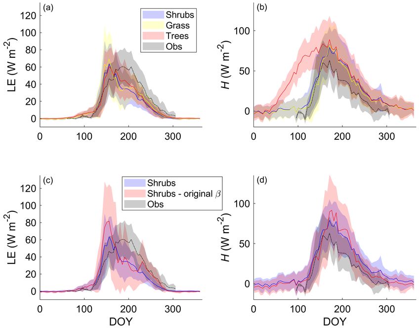
snow-free earlier than observations by 3 ± 4 d (mean ± SD) Differences in LE between the shrub, grass, and tree PFT
with a range of 11 d earlier to 5 d later. simulations were relatively small on average (Fig. 4a). The
Modelled mean daily relative VWC for the top soil layer adoption of the Merlin et al. (2011) β formulation reduced
(0–10 cm) averaged over 2004–2017 agreed reasonably well overestimation of LE by approximately 30 % during and just
with relative VWC measured at 7 cm depth (Fig. 3a). Al- after snowmelt (mid-May to mid-June) (Fig. 4c). In sum-
though interannual variability was high, VWC tended to be mer, the new β formulation greatly reduced variability in
overestimated by the model around snowmelt and underes- LE and ensured there were no summer dates with unrealis-
timated later in the growing season (early August to mid- tically low LE (Fig. 4c). However, all three PFT simulations
October) regardless of PFT simulation. At the end of the with the new β formulation still overestimated LE during and
growing season, the shrub simulation represented VWC the just after snowmelt and underestimated LE in summer (start-
best; modelled relative VWC was lower than observed by ing in late June). Average annual LE was 514, 397, 430, and
0.09, 0.17, and 0.18 m3 m−3 for the shrub, grass, and tree 434 MJ m−2 (or 16.3, 12.6, 13.6, and 13.8 W m−2 d−1 on av-
PFT simulations, respectively. Simulated end-of-growing- erage) for the observations, shrub simulations, grass simula-
season relative VWC for the 10–20 cm layer was lower than tions, and tree simulations, respectively. The observed annual
observed by 0.11, 0.26, and 0.27 m3 m−3 for the shrub, grass, value only includes data from DOY 95–310 as observations
and tree PFT simulations, respectively. The original β for- were not available for the whole year, but model results sug-
mulation, which was known to overestimate ground evapora- gest that LE during the missing time period likely contributed
tion (Sun and Verseghy, 2019), greatly underestimated rela- very little (< 2 %) to the annual total.
tive VWC by on average 0.23 m3 m−3 for the top soil layer ET as simulated by the shrub PFT with the new β was
dominated by ground evaporation (E) until mid-June, peak-
ing shortly after snowmelt (Fig. 5). Ground E was slightly
https://doi.org/10.5194/bg-18-3263-2021 Biogeosciences, 18, 3263–3283, 20213272 G. Meyer et al.: Simulating high-latitude shrubs at a dwarf-shrub tundra site
Figure 1. Mean 5 d average soil temperature for layer 1 (0–10 cm depth), 3 (20–30 cm depth), and 6 (50–60 cm depth) of the shrub simulations
using the new (Merlin et al., 2011) and original β (Lee and Pielke, 1992) formulation compared to measurements at 5, 25, and 60 cm depth,
respectively, averaged over 2004–2017. Shaded areas show the standard deviation of the daily mean for 2004–2017.
Figure 2. Mean observed and modelled 5 d average snow depth av-
eraged over 2004–2017 for the shrub simulation. Shaded areas show
the standard deviation of the daily mean for 2004–2017.
higher for the grass simulation and slightly lower for the
tree simulation in spring compared to the shrub simulation
(Fig. 5). Transpiration (T ) was an important contributor to
ET from mid-June to early September, peaking in early Au-
gust. Maximum T was 40 %–45 % greater for the grass and Figure 3. Mean 5 d average simulated relative volumetric water
tree PFT simulations compared to the shrub PFT simula- content (VWC, m3 m−3 ; see Eq. 11) (a) for the top model soil layer
tion (Fig. 5), resulting in slightly greater ET (also shown as (0–10 cm depth) and observations at 7 cm depth and (b) for the sec-
greater LE in Fig. 4a). For all three simulations, E of water ond layer (10–20 cm depth) and observations measured at 20 cm
intercepted by the canopy was a minor component of total depth averaged over 2004–2017 for the shrub, grass, and tree sim-
ET. ulations. For the shrub simulation, results using the new (Merlin
For H , the shrub and grass simulations were similar, et al., 2011) and original β (Lee and Pielke, 1992) formulation are
but the tree simulation greatly overestimated H especially shown. Measurements at the 20 cm depth were only available start-
from mid-April to the end of May (Fig. 4b). The aver- ing late August 2015, while measurements at the 7 cm depth began
in June 2004. Shaded areas show the standard deviation for 2004–
age annual total H for the tree simulation (1046 MJ m−2
2017 for the model results and observations at 7 cm depth and for
or 33.2 W m−2 d−1 ) was about 1.5 times as large as for the 2015–2017 for observations at 20 cm depth.
shrub (659 MJ m−2 or 20.9 W m−2 d−1 ) and grass simula-
tions (605 MJ m−2 or 19.2 W m−2 d−1 ) and more than 2.6
times the observed value (398 MJ m−2 or 12.6 W m−2 d−1
Biogeosciences, 18, 3263–3283, 2021 https://doi.org/10.5194/bg-18-3263-2021G. Meyer et al.: Simulating high-latitude shrubs at a dwarf-shrub tundra site 3273
ing season uptake that was 43 g C m2 larger than observa-
tions (Table 5). In contrast, simulated total growing season
Re agreed well with observations (Table 5), although it was
slightly higher than observed in spring and lower in summer
(Fig. 6).
NEP simulated with the grass PFT lagged observations in
the spring, peaking on average 49 d after the observations
(Fig. 6a). Summer maximum GPP for the grass simulation
was higher and, on average, reached a daily maximum 9 d
later than observations. Simulated grass PFT GPP continued
late into the fall, when observed GPP had declined to near
zero. Total Re was similar (Table 5) to Re simulated with the
shrub PFT, but again seasonal trends were offset by on aver-
age 10 d.
For the tree PFT simulation, simulated NEP and GPP were
reasonably close to the measured values in the spring, al-
though the start of NEP uptake was still about 10 d early
Figure 4. Mean 5 d average (a) latent (LE) and (b) sensible heat flux (Fig. 6). Uptake was overestimated in mid-summer and into
(H ) over 2004–2017 for the shrub, grass, and tree simulations using
the fall compared to measurements, resulting in the largest
the new β formulation (Merlin et al., 2011) and (c) LE and (d) H
growing season NEP (Table 5).
using the new and the original β formulation (Lee and Pielke, 1992)
along with EC tower observations. Shaded areas show the standard Both chamber and EC measurements show a more rapid
deviation of the daily mean for 2004–2017. decrease in CO2 emissions throughout September than shrub
PFT simulations, as soil and air T dropped to or below 0 ◦ C
(Fig. 6). However, EC flux observations in October and early
for the period DOY 95–310). Only considering the time November (DOY 275–309) were well represented by the
period where measurements were available, average H for NEP simulated using the shrub PFTs (Fig. 6). During the
the tree simulation was still 2.3 times the observed value. winter, from early November through March, when there
The original β formulation and shrub PFT simulation de- were no EC measurements (DOY 310–365 and DOY 1–
creased H throughout the year except in summer, so it 76), all three simulations had lower NEP and higher Re
had relatively little impact on the annual H (592 MJ m−2 than observed fluxes from the chambers (Fig. 6). However,
or 18.8 W m−2 d−1 ) compared with the new β formulation the chamber-based observations have some significant uncer-
(659 MJ m−2 or 20.9 W m−2 d−1 ). tainties as fluxes were measured over one winter (fall 2018–
These large differences in spring H among PFT simula- spring 2019) only, which was outside the simulation period
tions could be linked to differences in simulated Rn (Fig. S6) of 2004–2017. In addition, forced diffusion chambers have
and albedo (not shown). Albedo and Rn were similar for the a much smaller footprint (41 cm2 ) with less diverse ground
shrub and grass simulations, with average albedo values of cover than the seasonal EC footprint of 10 ha or more.
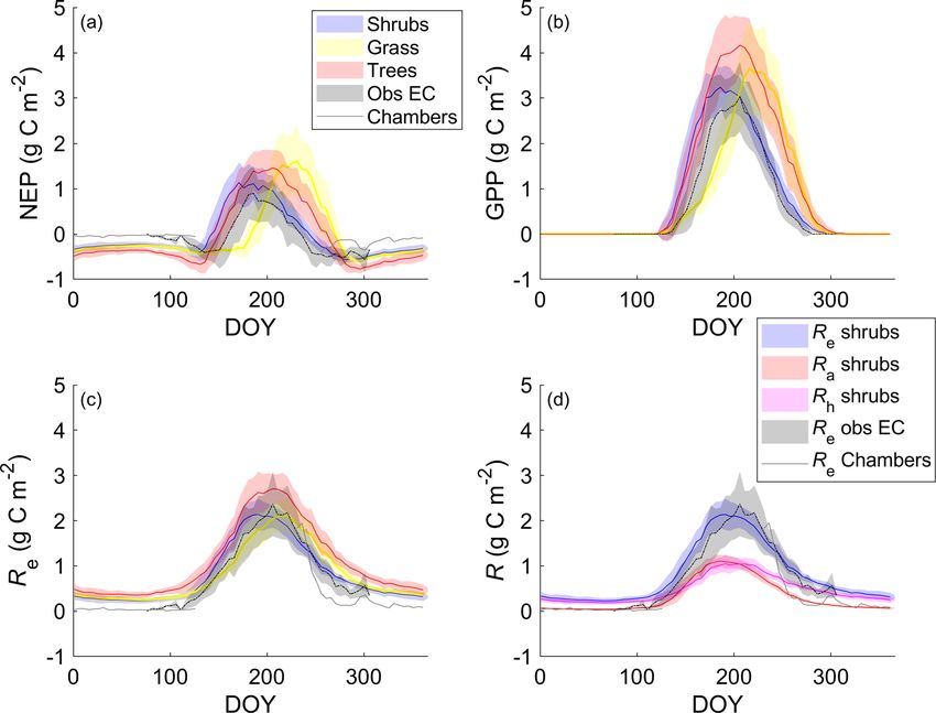
0.91 and 0.92, respectively, during late winter, which was During summer, the shrub simulation’s Ra and Rh were
only slightly lower than the observed value of 0.97. The tree roughly half of Re (Fig. 6d). Fall and winter CO2 emissions
simulation, however, had a much larger Rn and lower albedo were primarily through Rh , although Ra remained above
(0.55) than the shrub and grass simulations during winter, as zero. Otherwise, Ra closely followed GPP trends. Similar
the tall trees cannot be buried by snow. patterns with slightly larger values were observed for the tree
simulation, while the grass simulation’s Ra was near zero for
3.4 Net ecosystem CO2 exchange and its component the winter months (Fig. S7).
fluxes All three model simulations suggest that DL1 was a net
source of CO2 over the 2004–2017 period (Fig. 7 and Ta-
The shrub PFT simulation with the new β formulation best ble 5). Winter and shoulder season CO2 emissions from
represented observed NEP and its component fluxes (Fig. 6 October to April exceeded May through September CO2
and Table 5). The new β formulation raised modelled VWC, uptake by 26 %–32 % on average for the three simula-
reduced water stress, and supported GPP rates that closely re- tions. Over the 14-year period, there was a net winter CO2
sembled GPP derived from field observations at DL1. In con- loss of 211 g C m−2 for grass, 254 g C m−2 for shrub, and
trast, the original β formulation resulted in GPP values that 344 g C m−2 for tree simulations, which was equal to an av-
were only 26 % of observed values (Table 5 and Fig. S4). erage annual NEP of −15 to −25 g C m−2 yr−1 (Table 5).
NEP simulated with the shrub PFT and new β formulation Bearing in mind the caveats discussed above regarding com-
nevertheless was overestimated in spring as GPP started ap- bining chamber and EC data streams, these simulated results
proximately 9 d earlier than observed, resulting in total grow- were similar to an estimated NEP of −17 g C m−2 yr−1 ob-
https://doi.org/10.5194/bg-18-3263-2021 Biogeosciences, 18, 3263–3283, 20213274 G. Meyer et al.: Simulating high-latitude shrubs at a dwarf-shrub tundra site
Figure 5. Mean 5 d average modelled evapotranspiration (ET) and its component fluxes (transpiration (T ), ground and canopy evaporation
(E)) along with observed ET averaged over 2004–2017 for the shrub, grass, and tree PFT simulations using the new β (Merlin et al., 2011)
formulation. Shaded areas show the standard deviation of the daily mean for 2004–2017.
Table 5. Mean ± SD annual and growing season (GS; 1 May–30 September) net ecosystem productivity (NEP), gross primary productivity
(GPP), and ecosystem respiration (Re ) averaged over 2004–2017 for the shrub simulations using the new (Merlin et al., 2011) and origi-
nal β (Lee and Pielke, 1992) formulation, for the grass and tree simulations, and for observations. Eddy covariance flux measurements were
not available through the winter and are only reported for the growing season. Standard deviations (SDs) for the observed and simulated
fluxes are calculated by error propagation of the SD of daily values.
Simulation NEP [g C m−2 ] GPP [g C m−2 ] Re [g C m−2 ]
Annual GS Annual GS Annual GS
Observations – 12 ± 5 – 214 ± 7 – 202 ± 5
Shrubs −18 ± 4 55 ± 4 276 ± 6 273 ± 6 294 ± 3 218 ± 3
Grass −15 ± 6 61 ± 6 279 ± 9 271 ± 8 295 ± 4 210 ± 3
Trees −25 ± 5 82 ± 5 374 ± 8 365 ± 8 399 ± 4 283 ± 4
Shrubs – original β −7 ± 2 9±2 57 ± 2 56 ± 2 64 ± 1 47 ± 1
tained using these two sets of flux observations at DL1. The the shrub simulation only showed annual net CO2 uptake in
estimate of annual NEP was calculated from the sum of EC- 2012.
based NEP (12 ± 5 g C m−2 ) for the 5-month growing season
(Table 5), EC-based NEP (−19 ± 1 g C m−2 ) for the 81 d that
EC flux data were available during the shoulder seasons, and 4 Discussion
chamber-based NEP (−10 g C m−2 ) for the 131 d that winter
Although we focus on high-latitude shrubs, shrubs are an im-
EC fluxes were not available (Fig. 6).
portant growth form in multiple regions and biomes; cover
The simulations of NEP differed in response to interannual
about 40 % of the land surface, including polar and alpine
variability in meteorological forcing (Table S2). On average,
tundra, arid regions, and wetlands; and are often dominant
the 2010–2017 growing season was 2.1 ◦ C warmer and over
within forest understories (Götmark et al., 2016). Shrubs, as
2 times wetter than 2004–2009 (two-tailed t-test p < 0.05)
a growth form, have a number of advantages compared to
(Table S2). NEP simulated using the grass PFT was more
small trees. For example, in disturbed and low-productivity
sensitive to these different weather conditions and thus more
areas, shrubs have higher growth rates and, having multiple
variable than the other two simulations over the study pe-
short or bendable stems, are more resilient to storm damage
riod, including a few years (2006, 2011, 2012, 2013, 2016,
and weight of snow loading and can more readily recover
and 2017) where DL1 was simulated to be a net CO2 sink.
from stem breakage and thus have higher survival rates un-
Annual net CO2 uptake was also simulated for a few years
der extreme conditions (Götmark et al., 2016).
(2011, 2012, 2013, and 2017) using the tree PFTs, while
Biogeosciences, 18, 3263–3283, 2021 https://doi.org/10.5194/bg-18-3263-2021You can also read