Assimilating synthetic Biogeochemical-Argo and ocean colour observations into a global ocean model to inform observing system design - Biogeosciences
←
→
Page content transcription
If your browser does not render page correctly, please read the page content below
Biogeosciences, 18, 509–534, 2021
https://doi.org/10.5194/bg-18-509-2021
© Author(s) 2021. This work is distributed under
the Creative Commons Attribution 4.0 License.

Assimilating synthetic Biogeochemical-Argo and ocean
colour observations into a global ocean model to inform
observing system design
David Ford
Met Office, FitzRoy Road, Exeter, EX1 3PB, UK

Correspondence: David Ford (david.ford@metoffice.gov.uk)

Received: 30 April 2020 – Discussion started: 15 May 2020
Revised: 30 November 2020 – Accepted: 7 December 2020 – Published: 21 January 2021

Abstract. A set of observing system simulation experiments          is re-usable under the Open Government Licence (OGL). The
was performed. This assessed the impact on global ocean             Creative Commons Attribution 4.0 License and the OGL are
biogeochemical reanalyses of assimilating chlorophyll from          interoperable and do not conflict with, reduce or limit each other.
remotely sensed ocean colour and in situ observations of
chlorophyll, nitrate, oxygen, and pH from a proposed ar-            © Crown copyright 2021
ray of Biogeochemical-Argo (BGC-Argo) floats. Two poten-
tial BGC-Argo array distributions were tested: one for which
biogeochemical sensors are placed on all current Argo floats        1   Introduction
and one for which biogeochemical sensors are placed on a
quarter of current Argo floats. Assimilating BGC-Argo data          Throughout the ocean, physical and chemical processes in-
greatly improved model results throughout the water col-            teract with a teeming ecosystem to affect all life on Earth.
umn. This included surface partial pressure of carbon dioxide       The upwelling of nutrient-rich waters fuels the growth of
(pCO2 ), which is an important output of reanalyses. In terms       phytoplankton, which form the base of the marine food web
of surface chlorophyll, assimilating ocean colour effectively       and contribute half the planet’s primary production (Field
constrained the model, with BGC-Argo providing no added             et al., 1998). Oxygen is required for marine and terrestrial
benefit at the global scale. The vertical distribution of chloro-   life, and its availability depends on ocean circulation, solubil-
phyll was improved by assimilating BGC-Argo data. Both              ity, and biological activity. Carbon is taken up at the sea sur-
BGC-Argo array distributions gave benefits, with greater im-        face, at a rate contingent on physics and biology, and trans-
provements seen with more observations. From the point of           ported throughout the ocean. Some is stored for centuries at
view of ocean reanalysis, it is recommended to proceed with         vast depths, mitigating climate change. Some is quickly re-
development of BGC-Argo as a priority. The proposed array           leased back to the atmosphere. All these phenomena are reg-
of 1000 floats will lead to clear improvements in reanalyses,       ulated by an array of processes which display variability on
with a larger array likely to bring further benefits. The ocean     a range of scales from milliseconds to millennia and from
colour satellite observing system should also be maintained,        nanometres to ocean basins.
as ocean colour and BGC-Argo will provide complementary                Understanding, monitoring, and predicting these processes
benefits.                                                           is key to addressing some of the biggest challenges facing hu-
                                                                    manity. Rising carbon dioxide (CO2 ) emissions are leading
                                                                    to climatic changes which threaten severe impacts on peo-
                                                                    ple and ecosystems (IPCC, 2014). Uptake of carbon by the
Copyright statement. The works published in this journal are
                                                                    global ocean acts to mitigate these impacts, but the ocean
distributed under the Creative Commons Attribution 4.0 License.
This license does not affect the Crown copyright work, which        carbon sink is highly variable and its future magnitude un-
                                                                    certain (McKinley et al., 2017). At the same time, when CO2

Published by Copernicus Publications on behalf of the European Geosciences Union.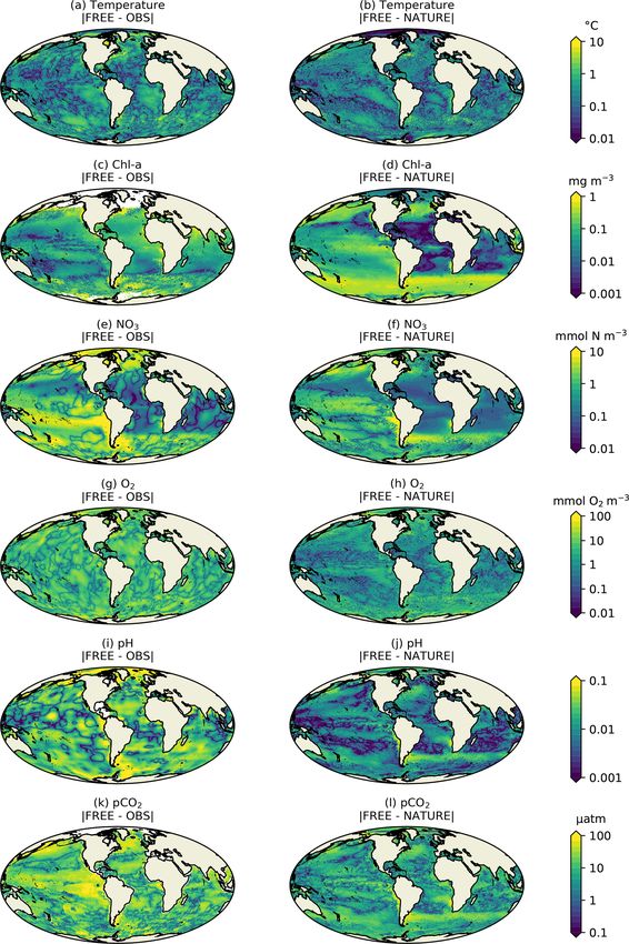
510                                  D. Ford: Assimilating synthetic Biogeochemical-Argo and ocean colour observations

dissolves in seawater it reacts with it, leading to a decrease   The aim is for all these floats to measure six core variables:
in pH referred to as ocean acidification (Doney et al., 2009).   oxygen concentration (O2 ), nitrate concentration (NO3 ), pH,
This could have major consequences for marine life, particu-     chlorophyll a concentration (Chl a), suspended particles, and
larly organisms which form calcium carbonate shells, which       downwelling irradiance. This promises to transform scien-
become at risk of dissolution if the seawater pH is too low.     tific understanding of ocean biogeochemistry. Thanks to a
Changes in climate and eutrophication also appear to be lead-    series of regional programmes, there are already over 300 op-
ing to expanding “dead zones” in the ocean (Diaz and Rosen-      erational floats measuring one or more biogeochemical vari-
berg, 2008; Altieri and Gedan, 2015), where oxygen concen-       ables. Few of these floats yet measure all the core BGC-Argo
trations are too low for most organisms to survive. On shorter   variables, and spatial coverage is highly uneven, but impor-
timescales, primary production varies considerably due to        tant scientific discoveries regarding phytoplankton, carbon,
natural climate variability such as the El Niño–Southern Os-     and nutrient dynamics have been made (Roemmich et al.,
cillation (ENSO), and changes can have profound impacts on       2019).
higher trophic levels and hence the fisheries and aquaculture        The value of observations can be further enhanced by com-
on which an estimated 12 % of the global population rely for     bining them with numerical models using data assimilation
their livelihoods (FAO, 2016). All these factors and more are    (Kalnay, 2003). Ocean colour data are increasingly assim-
captured in a drive towards the “good environmental status”      ilated in state-of-the-art reanalysis (Rousseaux and Gregg,
of national waters, as regulated by policies such as the Ma-     2015; Ciavatta et al., 2016; Ford and Barciela, 2017) and
rine Strategy Framework Directive (MSFD) of the European         forecasting (Teruzzi et al., 2014; Skákala et al., 2018) sys-
Union (EU).                                                      tems. This has consistently been shown to improve simula-
   Comprehensively monitoring all relevant processes in the      tions of phytoplankton, but the impact on other model vari-
global ocean, and their variability and trends, is not a triv-   ables, especially for the subsurface, is limited (Gehlen et al.,
ial task. For ocean biogeochemistry, the global observing        2015). Physical data assimilation has the potential to im-
system consists of various components which, while often         prove biogeochemistry but has often been found to have the
sparse and disparate, have allowed fundamental insights.         opposite effect due to spurious impacts on vertical mixing
More than 2 decades of routine satellite ocean colour data       to which biogeochemical variables are particularly sensitive
(Groom et al., 2019) have yielded unprecedented knowl-           (Park et al., 2018; Raghukumar et al., 2015). Assimilating
edge about phytoplankton variability (Racault et al., 2017)      multivariate in situ biogeochemical data should help address
and even helped overturn decades of scientific consensus on      these issues and greatly improve reanalyses and forecasts (Yu
bloom formation (Behrenfeld and Boss, 2014). In situ sta-        et al., 2018), but due to the sparsity of observational cover-
tions such as the Bermuda Atlantic Time Series (BATS) have       age, efforts have largely been limited to parameter estimation
allowed long-term monitoring of multiple variables at fixed      (Schartau et al., 2017), 1-D models (Torres et al., 2006), in-
locations (Bates et al., 2014), and various networks of ships,   dividual research cruises (Anderson et al., 2000), or surface-
gliders, and moorings give ongoing views of different aspects    only carbon data (Valsala and Maksyutov, 2010; While et al.,
of the global ocean (Telszewski et al., 2018). These observa-    2012). Furthermore, in situ biogeochemical observations are
tion networks are vital and have transformed our understand-     rarely available in near-real time, limiting their suitability for
ing of ocean biogeochemistry. But they remain sparse, and        operational applications.
coverage is insufficient to address all outstanding scientific       The increasing availability of BGC-Argo data promises
questions or provide comprehensive monitoring on a global        to change this, with great potential for improving reanaly-
scale.                                                           ses and forecasts (Fennel et al., 2019). For instance, BGC-
   Observation of ocean physics has been revolutionised by       Argo observations of O2 have been assimilated by Verdy
the advent of Argo (Roemmich et al., 2019). A global array       and Mazloff (2017), who produced a 5-year state estimate
of around 4000 autonomous floats drift at a typical parking      of the Southern Ocean using an adjoint method, and were
depth of 1000 m, and every 10 d they descend to 2000 m be-       able to capture over 60 % of the variance in oxygen pro-
fore rising to the surface, profiling temperature and salinity   files at 200 and 1000 m of depth. Furthermore, Cossarini
as they do so. The data are then transmitted to satellites in    et al. (2019) assimilated BGC-Argo profiles of Chl a into a
near-real time before the float returns to its parking depth.    model of the Mediterranean Sea and found this was success-
Argo has facilitated breakthroughs in climate science (Wijf-     ful in adjusting the shape of chlorophyll profiles and that with
fels et al., 2016) and improvements in physical ocean reanal-    the present number of BGC-Argo floats they could constrain
yses and forecasts (Davidson et al., 2019).                      phytoplankton dynamics in up to 10 % of the Mediterranean
   The Argo initiative is now being extended to biogeochem-      Sea.
istry through the Biogeochemical-Argo (hereafter BGC-                This paper describes the development of a scheme to as-
Argo) programme (Biogeochemical-Argo Planning Group,             similate profiles of Chl a, NO3 , O2 , and pH into an updated
2016; Roemmich et al., 2019). In the next decade, it is          version of the Met Office’s global physical–biogeochemical
planned to establish a global array of 1000 BGC-Argo floats,     ocean reanalysis system. A set of observing system simu-
which are Argo floats equipped with biogeochemical sensors.      lation experiments (OSSEs) (Masutani et al., 2010) is pre-

Biogeosciences, 18, 509–534, 2021                                                     https://doi.org/10.5194/bg-18-509-2021
D. Ford: Assimilating synthetic Biogeochemical-Argo and ocean colour observations                                            511

sented to assess the potential value of different numbers         with the physics version of the data assimilation scheme de-
of BGC-Argo floats. The work forms part of a coordinated          scribed below, the ocean and sea ice models are also used
effort within the EU Horizon 2020 research project At-            in version 14 of the Forecasting Ocean Assimilation Model
lantOS (https://www.atlantos-h2020.eu, last access: 18 Jan-       (FOAM), earlier versions of which are described by Blockley
uary 2021). Four groups performed OSSEs assessing physics         et al. (2014) and Storkey et al. (2010). FOAM is run opera-
observations, the results of which have been synthesised by       tionally at the Met Office to produce short-range forecasts
Gasparin et al. (2019). Two groups performed OSSEs as-            of the physical ocean and sea ice state. It is also used to
sessing biogeochemistry: Germineaud et al. (2019) and this        initialise the ocean and sea ice components of the Met Of-
study. Germineaud et al. (2019) presented a probabilistic         fice Global Seasonal forecasting system version 5 (GloSea5)
evaluation at a single assimilation time step, finding that       (MacLachlan et al., 2015; Scaife et al., 2014) and short-range
Chl a from BGC-Argo floats added value at surface locations       coupled ocean–atmosphere forecasting system (Guiavarc’h
where ocean colour was unavailable and at depth.                  et al., 2019).
   The biogeochemistry OSSEs consider two potential sce-             The biogeochemical ocean model used in this study is ver-
narios: (1) a global BGC-Argo array equivalent to having          sion 2 of the Model of Ecosystem Dynamics, nutrient Util-
biogeochemical sensors on one in four existing Argo floats,       isation, Sequestration and Acidification (MEDUSA) (Yool
which is comparable to the planned target of 1000 floats, and     et al., 2013). MEDUSA is of intermediate complexity, rep-
(2) a global BGC-Argo array equivalent to having biogeo-          resenting two phytoplankton and two zooplankton types as
chemical sensors on all existing Argo floats. The aims were       well as the cycles of nitrogen, silicon, iron, carbon, and oxy-
to assess the impact on reanalysis and forecasting systems        gen. This differs from previous versions of the Met Office
that might be seen by assimilating multivariate BGC-Argo          physical–biogeochemical ocean reanalysis system (Ford and
data, the influence of array size, and the value BGC-Argo         Barciela, 2017), which used the Hadley Centre Ocean Car-
would add to the existing ocean colour satellite constellation.   bon Cycle Model (HadOCC) (Palmer and Totterdell, 2001).
Assimilation of physics variables was not included due to the     This is because, following an intercomparison (Kwiatkowski
issues mentioned above, reflecting the way state-of-the-art       et al., 2014) of biogeochemical models developed in the
biogeochemical reanalyses are run (Fennel et al., 2019).          UK, MEDUSA was chosen to be the ocean biogeochemi-
   This paper describes the updated model, newly developed        cal component of version 1 of the UK Earth System Model
assimilation scheme, and set-up of the OSSEs. Results are         (UKESM1) (Sellar et al., 2019). UKESM1 consists of a
then presented showing the impact of assimilating the two         lower-resolution version of GC3.1 coupled with models of
potential BGC-Argo arrays, with and without ocean colour          ocean biogeochemistry, atmospheric chemistry and aerosols,
data. Finally, recommendations are made for the future de-        and ice sheets, and it is used for Earth system climate simu-
velopment of observing and assimilation systems.                  lations submitted to CMIP6. Using the same model versions
                                                                  for forecasting, reanalysis, and climate simulations provides
                                                                  a seamless framework for simulating the Earth system (Mar-
2     Model and assimilation                                      tin et al., 2010).

The reanalysis system is an upgraded version of that used         2.2     Assimilation
in previous biogeochemical data assimilation studies at the
Met Office (Ford et al., 2012; While et al., 2012; Ford and       2.2.1    Overview
Barciela, 2017; Ford, 2020).
                                                                  The data assimilation scheme used here is version 5 of
                                                                  NEMOVAR (Weaver et al., 2003, 2005; Mogensen et al.,
2.1    Model
                                                                  2009, 2012), following the implementation for assimilat-
                                                                  ing physical variables into the global FOAM system (Wa-
The physical ocean model used is the GO6 configuration
                                                                  ters et al., 2015) and for assimilating ocean colour data
(Storkey et al., 2018) of the Nucleus for European Mod-
                                                                  into HadOCC (Ford, 2020) and the European Regional Seas
elling of the Ocean (NEMO) hydrodynamic model (Madec,
                                                                  Ecosystem Model (ERSEM) (Skákala et al., 2018, 2020).
2008) with the extended ORCA025 tripolar grid, which has
                                                                  As detailed in Waters et al. (2015), this implementation of
a horizontal resolution of 1/4◦ and 75 vertical levels. This
                                                                  NEMOVAR uses a first guess at appropriate time (FGAT)
is coupled online to the GSI8.1 configuration (Ridley et al.,
                                                                  3D-Var methodology. A conjugate gradient algorithm is used
2018) of the Los Alamos Sea Ice Model (CICE) (Hunke
                                                                  to iteratively minimise the cost function
et al., 2015). Together, these form the ocean and sea ice com-
ponents of the GC3.1 configuration (Williams et al., 2017)                1             1
of the Hadley Centre Global Environment Model version 3           J (δx) = δx T B−1 δx + (d − Hδx)T R−1 (d − Hδx), (1)
                                                                          2             2
(HadGEM3), which is used for physical climate simulations
submitted to the Coupled Model Intercomparison Project            where the increment δx = x − x b is the difference between
Phase 6 (CMIP6) (Eyring et al., 2016). When combined              the state vector x and its background estimate x b ; the inno-

https://doi.org/10.5194/bg-18-509-2021                                                     Biogeosciences, 18, 509–534, 2021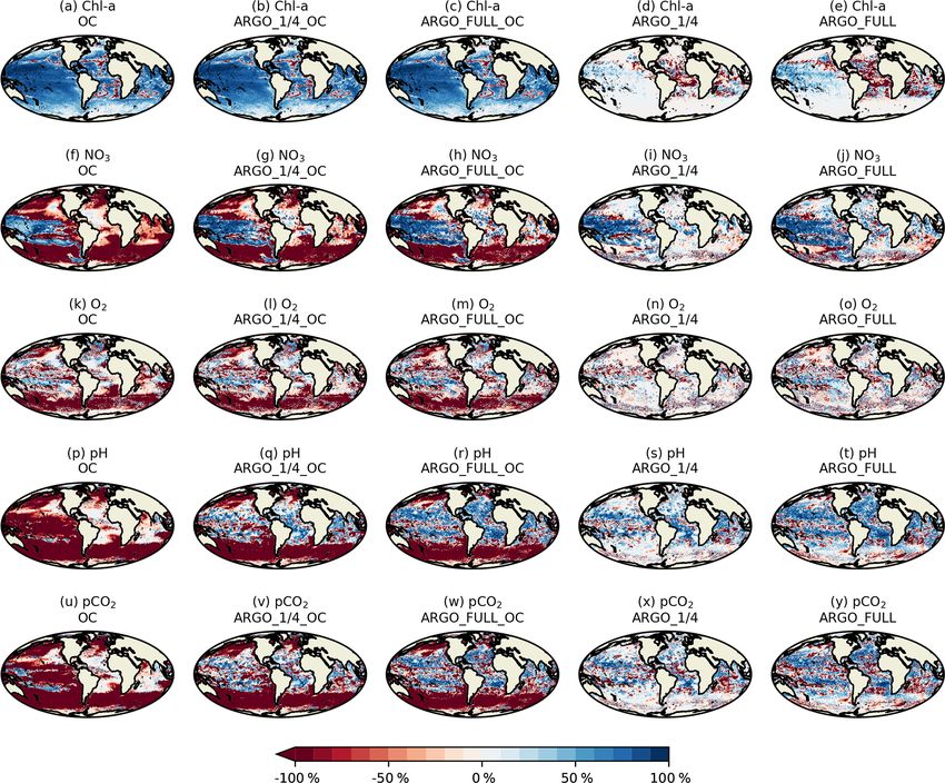
512                                    D. Ford: Assimilating synthetic Biogeochemical-Argo and ocean colour observations

vation vector d = y −H(x i ) is the difference between the ob-      tribution (Campbell, 1995). The background and observation
servation vector y and x i = Mt0 →ti (x b ), where Mt0 →ti is the   error covariances used were the same as in Ford (2020). In
nonlinear propagation model that propagates the background          the horizontal, a correlation length scale based on the first
state to the state at time i, operated on by the observation op-    baroclinic Rossby radius was used, varying from a value of
erator H; H is the linearised observation operator; B is the        25 km at low latitudes to 150 km at the Equator, consistent
background error covariance matrix; and R is the observa-           with Waters et al. (2015).
tion error covariance matrix. A diffusion operator is used to          For surface data, such as ocean colour, NEMOVAR can be
efficiently model spatial correlations (Mirouze and Weaver,         applied in one of two ways. The first, which is computation-
2010; Mirouze et al., 2016). A total of 10 iterations of the        ally most efficient and has been used in previous ocean colour
diffusion operator are applied, simulating the matrix multi-        assimilation studies (Ford, 2020; Skákala et al., 2018, 2020),
plication of an autoregressive correlation matrix, which pro-       is to calculate a set of 2-D surface increments which are ap-
vides a good approximation to a Gaussian correlation func-          plied equally through the mixed layer. The second is to cal-
tion (Waters et al., 2015). The observation operator forms          culate a set of 3-D increments with information from the sur-
part of the NEMO code and computes model values in ob-              face observations propagated downwards using vertical cor-
servation space by interpolating model fields to observation        relation length scales, as described by Waters et al. (2015)
locations at the closest model time step to the time each ob-       for physical variables. The subsurface background error stan-
servation was made. The observation operator was extended           dard deviations are parameterised based on the vertical gra-
in this study to work for 3-D biogeochemical variables in ad-       dient of density with depth to allow a flow-dependent vertical
dition to physical variables.                                       structure to the errors. The vertical correlation length scale is
   When applied to physics data, NEMOVAR decomposes                 dependent on the model’s mixed layer depth, as determined
the full multivariate background error covariance matrix into       from a 1 d model forecast. At the surface, the vertical correla-
an unbalanced and a balanced component for each variable.           tion length scale is set to the depth of the mixed layer so that
The unbalanced component considers the uncorrelated com-            information from surface observations is spread to the base
ponent of each variable using univariate error covariances,         of the mixed layer but not below it. The latter method allows
while the balanced component considers correlations be-             satellite and in situ profile observations of a given variable to
tween variables. The balanced component is derived using            be consistently combined by NEMOVAR to produce a single
a set of linearised balance operators based on physical rela-       set of 3-D increments for that variable and was therefore the
tionships (Weaver et al., 2005; Mogensen et al., 2012). In this     method employed in this study.
study, NEMOVAR has been applied to biogeochemical vari-                This gives a set of 3-D log10 (Chl a) increments on the
ables with no multivariate relationships applied, and the cost      model grid, which must be applied to the model. The
function is minimised separately for each assimilated vari-         log10 (Chl a) increments were converted to Chl a increments
able. Development of biogeochemical balance relationships           using the background total Chl a and split between diatoms
within NEMOVAR could be expected to bring improved re-              and non-diatoms so as to conserve the ratio between the two
sults, but this would be a major development to NEMOVAR.            in the background model field. Phytoplankton biomass was
The aim of this study was to develop an initial implementa-         then similarly updated to conserve the stoichiometric ratios
tion that could be used with BGC-Argo data, and that can be         in the background field, following the approach of Teruzzi
further developed as systems mature.                                et al. (2014) and Skákala et al. (2018, 2020).
   All increments are applied to the model over 1 d using in-
cremental analysis updates (IAU) (Bloom et al., 1996), which
                                                                    2.2.3   BGC-Argo
apply an equal proportion of the increments at each model
time step, in order to reduce initialisation shocks.
   NEMOVAR is used in this study to assimilate simu-                For in situ profiles of biogeochemistry, as might be obtained
lated ocean colour and BGC-Argo data, as described in               from BGC-Argo, sets of 3-D increments were calculated for
the following sections. NEMOVAR can be used for com-                each assimilated variable, following the physics implementa-
bined physical–biogeochemical assimilation (Ford, 2020),            tion of Waters et al. (2015). The method was the same as for
but physics data were not assimilated in this study.                calculating 3-D ocean colour increments, as described above.
                                                                    The vertical correlation length scale was flow-dependent and
2.2.2   Ocean colour                                                varied with depth, as detailed by Waters et al. (2015). At the
                                                                    surface the vertical correlation length scale was set to the
NEMOVAR was used here to assimilate total surface                   depth of the mixed layer, decreasing to a minimum value
log10 (Chl a) from ocean colour. Since MEDUSA simulates             at the base of the mixed layer. This minimised the spread
Chl a for two phytoplankton types, diatoms and non-diatoms,         of information across the pycnocline due to the lack of cor-
these were summed by the observation operator to give total         relation of water mass properties in and below the mixed
Chl a to match the input observations. Log transformation           layer (Waters et al., 2015; Fontana et al., 2013). Below the
was performed in order to give a more Gaussian error dis-           mixed layer, the vertical correlation length scale increased

Biogeosciences, 18, 509–534, 2021                                                       https://doi.org/10.5194/bg-18-509-2021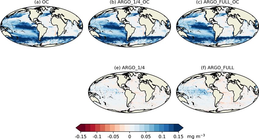
D. Ford: Assimilating synthetic Biogeochemical-Argo and ocean colour observations                                           513

with depth, proportional to the increase in vertical model grid     – a “nature run”, which is a realistic non-assimilative
spacing that occurs with depth.                                       model simulation of the real world that provides a
   In this study Chl a, NO3 , O2 , and pH were assimilated,           “truth” against which to validate the assimilative model;
but the methodology is simple to extend to other model vari-
ables. As for ocean colour assimilation, Chl a is the sum of        – synthetic observations representing both existing rou-
diatom and non-diatom Chl a, and a log transformation was             tine observations and future observing networks, which
performed prior to assimilation. As described above, assim-           are sampled from the nature run with appropriate errors
ilation of Chl a from ocean colour and in situ profiles can           prescribed;
be combined. NO3 and O2 are state variables in MEDUSA,
                                                                    – optionally, a free run, which provides an alternative
taking NO3 to be equivalent to the MEDUSA dissolved in-
                                                                      model simulation of the nature run period;
organic nitrogen (DIN) variable, while pH is a diagnostic
variable calculated using version 2.0 of the mocsy carbon-          – an assimilative run, which assimilates synthetic obser-
ate package (Orr and Epitalon, 2015), which implements the            vations representing existing routine observations into
SolveSAPHE algorithm (Munhoven, 2013) for solving the                 the alternative model simulation;
alkalinity–pH equation.
   The Chl a increments were applied using the stoichiomet-         – one or more additional versions of the assimilative run
ric balancing method described for ocean colour above. The            which also assimilate synthetic observations represent-
NO3 increments were directly applied to the MEDUSA DIN                ing the future observing networks under consideration;
variable and the O2 increments to the O2 variable. As pH is a         and
diagnostic variable, the pH increments cannot be applied di-
rectly. The approach taken to the assimilation of partial pres-     – assessment of the impact on reanalysis or forecast skill
sure of CO2 (pCO2 ) into HadOCC (While et al., 2012) was              of assimilating these observations by validating against
therefore adopted here with pH. In HadOCC, pCO2 is a func-            the nature run.
tion of temperature, salinity, dissolved organic carbon (DIC),
and alkalinity, and at constant temperature and salinity con-        One of the keys to obtaining informative results from an
stant lines of pCO2 are found in DIC / alkalinity space (see      OSSE is to ensure that all sources of error are appropriately
Fig. 1 of While et al., 2012). The scheme of While et al.         accounted for (Halliwell et al., 2014, 2017; Hoffman and At-
(2012) assumes that temperature and salinity are error-free       las, 2016). If the free run is more similar to the nature run
(and can be directly updated by physical data assimilation if     than the real forecasting system is to the real world, then it
not) and therefore updates DIC and alkalinity. As there is        can become easier for the assimilative system to recover the
no unique combination of DIC and alkalinity that gives a          truth, and the impact of the observing networks may be in-
specific pCO2 value, the smallest combined change to DIC          correctly estimated. As such, three general OSSE approaches
and alkalinity is made in order to reach the target pCO2          have been developed, which differ in how the free run varies
value. The same approach was taken here with pH, which            from the nature run.
in MEDUSA is a function of temperature, salinity, nutri-
                                                                    – In “identical twin experiments”, the nature and free runs
ents, latitude, depth, DIC, and alkalinity. In DIC / alkalinity
                                                                      differ only in their initial conditions. This set-up was
space, locally constant lines of pH are found when consid-
                                                                      frequently used in early OSSEs, but as most sources of
ering the range of present oceanic conditions (see Fig. 1a of
                                                                      model error are neglected, the results were found to be
Munhoven, 2013). The scheme developed here therefore up-
                                                                      overly optimistic, and the approach is no longer widely
dates DIC and alkalinity, assuming the other contributors to
                                                                      recommended (Arnold and Dey, 1986).
pH to be error-free, by making the smallest combined change
which would give the target pH.                                     – In “fraternal twin experiments”, the same model is still
                                                                      used for both the nature and free run, but more aspects
3     Observing system simulation experiments (OSSEs)                 are modified. These could include the initial conditions,
                                                                      lateral and surface boundary conditions, parameterisa-
3.1    Overview                                                       tions, and resolution. This takes much better account of
                                                                      model errors, and the approach is recommended over
As detailed by Masutani et al. (2010), OSSEs provide a way            identical twin experiments (Arnold and Dey, 1986; Ma-
to test the impact on forecasts and reanalyses of assimilat-          sutani et al., 2010; Yu et al., 2019).
ing observations which do not yet exist by using synthetic
observations. An OSSE typically comprises the following el-         – In “full OSSEs”, significantly different models are used
ements:                                                               for the nature and free runs in order to make the two
                                                                      more independent. The nature run is often run either at
                                                                      higher resolution than the assimilative model or with
                                                                      significantly different parameterisations (Fujii et al.,

https://doi.org/10.5194/bg-18-509-2021                                                     Biogeosciences, 18, 509–534, 2021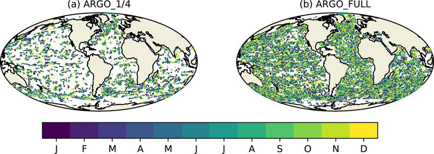
514                                   D. Ford: Assimilating synthetic Biogeochemical-Argo and ocean colour observations

Figure 1. Simulated BGC-Argo float trajectories for 2009 equivalent to having biogeochemical sensors on (a) one in four Argo floats and
(b) all Argo floats. Colours represent the month in which each observation is valid.

      2019). It is recommended to use this approach if pos-             The free run was performed for the same period, includ-
      sible (Masutani et al., 2010), but it relies on having two      ing spin-up, but differed from the nature run in the following
      appropriately different models available, which is not          ways.
      always the case.
                                                                        – Atmospheric boundary conditions were taken from the
   Due to the lack of availability of an appropriate alter-               JRA-55 reanalysis (Kobayashi et al., 2015).
native model for the nature run, it was decided within At-
                                                                        – NEMO initial conditions were taken from an earlier date
lantOS to take a fraternal twin approach for the biogeochem-
                                                                          (1 January 1999) of the hindcast of Storkey et al. (2018).
ical OSSEs. This is sufficient to account for most sources of
error, as long as any limitations of the approach are consid-           – MEDUSA initial conditions were taken from an ear-
ered when drawing and acting upon conclusions.                            lier year (1218) of the UKESM1 ocean-only spin-up,
                                                                          with DIC and alkalinity taken from the end of the non-
3.2   Model formulation                                                   assimilative 1/4◦ resolution experiment of Ford (2020).
The nature run in this study was run from 1 January 2008                – The NEMO parameter rn_efr, which affects near-
to 31 December 2009 using the default parameterisations for               inertial wave breaking and therefore vertical mixing
the model versions used. This is intended to be the best avail-           (Calvert and Siddorn, 2013), was increased from 0.05
able non-assimilative model representation of the real world.             to 0.1.
Validation of the general performance of the different system
components can be found in the references given in Sect. 2,             – The scheme used for advection of biogeochemical
and validation of the nature run is presented in Sect. 4.1. At-           variables was changed from total variance dissipa-
mospheric boundary conditions were taken from the ERA-                    tion (TVD) (Zalesak, 1979) to the monotone upstream
Interim reanalysis (Dee et al., 2011). Initial conditions for             scheme for conservative laws (MUSCL) (Van Leer,
NEMO were taken from the end of a 30-year hindcast of GO6                 1977; Lévy et al., 2001).
(Storkey et al., 2018). Initial conditions for CICE were taken          – An alternative set of MEDUSA parameters was used,
from a pre-operational trial of the FOAM v14 system. Initial              specifically parameter set 3 from Table 2 of Hemmings
conditions for MEDUSA were based on year 5000 of the ini-                 et al. (2015), which was found to give differences of an
tial ocean-only phase of the spin-up of UKESM1 for use in                 appropriate magnitude.
CMIP6 projections (Yool et al., 2020). As the UKESM1 spin-
up was run at 1◦ resolution with pre-industrial atmospheric              Together, these modifications generate approximations to
CO2 concentrations, the UKESM1 fields were interpolated               the errors that exist in atmospheric fluxes and simulations of
to 1/4◦ resolution, and the DIC and alkalinity fields were re-        ocean physics and biogeochemistry. It is important to mod-
placed by the contemporary model estimates used to initialise         ify all of these, as errors in atmosphere and ocean physics
the 1/4◦ resolution experiments in Ford (2020). To allow the          have significant impacts on biogeochemical reanalyses and
model to settle, the first year of the nature run was treated as      forecasts, and these errors must be accounted for if realistic
spin-up. The period was chosen to match OSSEs of the in situ          conclusions are to be drawn from the OSSEs.
physics observing system performed at the Met Office (Mao
et al., 2020) and more widely as part of AtlantOS (Gasparin           3.3   Synthetic observations
et al., 2019).
                                                                      Synthetic ocean colour and BGC-Argo observations were
                                                                      generated from the nature run for each day of 2009. Total

Biogeosciences, 18, 509–534, 2021                                                         https://doi.org/10.5194/bg-18-509-2021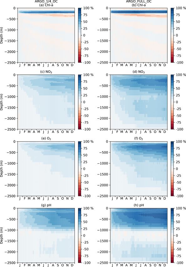
D. Ford: Assimilating synthetic Biogeochemical-Argo and ocean colour observations                                                515

Figure 2. Monthly mean surface (a–c) temperature, (d–f) Chl a, (g–i) NO3 , (j–l) O2 , (m–o) pH, and (p–r) pCO2 for December 2009 from
real-world observation-based products (left column), NATURE (middle column), and FREE (right column).

Chl a from ocean colour represents the current observing             ocean colour products (MODIS, OLCI, and VIIRS). BGC-
network typically assimilated in biogeochemical reanalyses           Argo float trajectories were based on Argo float trajectories
(Fennel et al., 2019). Observations were simulated at the            (Argo, 2000) used for physics OSSEs within AtlantOS (Gas-
same locations that were actually observed in 2009 in ver-           parin et al., 2019). These were generated using recent real
sion 3.1 of the ESA Climate Change Initiative (CCI) level 3          Argo float trajectories, with modifications to ensure more
daily merged sinusoidal grid product (Sathyendranath et al.,         even geographic coverage – for details see Gasparin et al.
2018, 2019), as used in recent Met Office reanalyses (Ford           (2019). In this study, for testing the scenario equivalent to
and Barciela, 2017). Whilst the products date from 2009              having biogeochemical sensors on all current standard Argo
rather than the present day, the observational coverage is           floats, the same “backbone” float trajectories were used as
similar, with three sensors contributing in 2009 (MERIS,             in the studies synthesised by Gasparin et al. (2019). For the
MODIS, and SeaWiFS) and three contributing to recent                 scenario equivalent to having biogeochemical sensors on one

https://doi.org/10.5194/bg-18-509-2021                                                         Biogeosciences, 18, 509–534, 2021
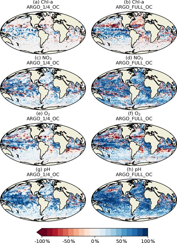
516                                      D. Ford: Assimilating synthetic Biogeochemical-Argo and ocean colour observations

Figure 3. Absolute difference for December 2009 for surface (a, b) temperature, (c, d) Chl a, (e, f) NO3 , (g–h) O2 , (i, j) pH, and (k, l) pCO2
between FREE and real-world observation-based products (left column), as well as between FREE and NATURE (right column).

in four Argo floats, these were subsampled using the last two             noise to the nature run values at observation locations using
digits of the float IDs. The geographic coverage in each case             standard deviations from the literature. A standard deviation
is shown in Fig. 1.                                                       of 30 % was agreed on within AtlantOS for Chl a from ocean
   In data assimilation, two components of observation er-                colour, a value commonly used in assimilation studies (Prad-
ror are typically considered: measurement error and repre-                han et al., 2020). The same value was used for BGC-Argo
sentation error (Janjić et al., 2018). Measurement error has             Chl a profiles, consistent with Boss et al. (2008). For the re-
been accounted for in this study by adding unbiased Gaussian              maining variables the values from Johnson et al. (2017) were

Biogeosciences, 18, 509–534, 2021                                                                https://doi.org/10.5194/bg-18-509-2021
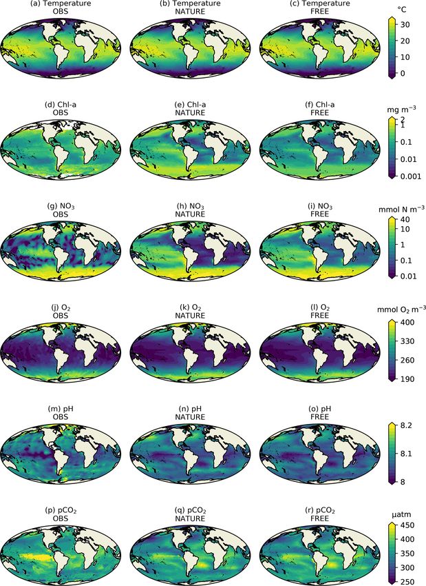
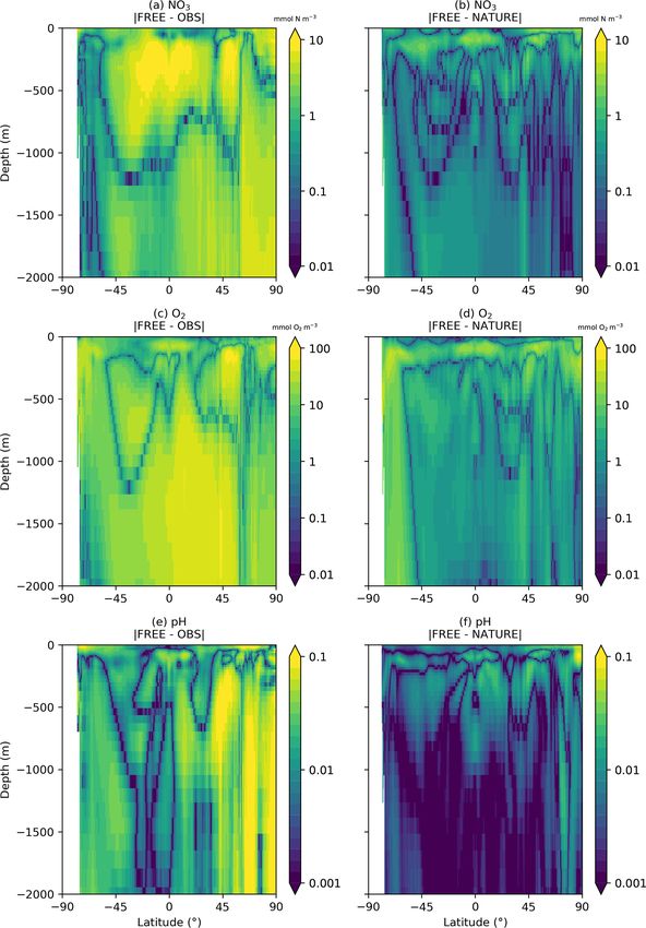
D. Ford: Assimilating synthetic Biogeochemical-Argo and ocean colour observations                                                517

Figure 4. Annual zonal mean sections of (a–c) NO3 , (d–f) O2 , and (g–i) pH from real-world observation-based products (a, d, g), NA-
TURE (b, e, h), and FREE (c, f, i).

used: 1 % for O2 , 0.005 for pH, and 0.5 mmol m−3 for NO3 .          physics OSSEs in AtlantOS (Gasparin et al., 2019). For each
To avoid generating spuriously noisy profiles, a single value        profile, the equivalent nature run values were calculated ei-
of Gaussian noise was calculated per profile rather than at          ther 3 d before or 3 d after, chosen at random. The difference
every depth level. Where the standard deviations used were a         between these and the truth value were taken to be the repre-
percentage, this was calculated using the mean of the profile.       sentation error and added to the observation values. The ad-
  Representation error arises from observations and models           vantage of this approach is that representation error is higher
representing differing spatial and temporal scales and pro-          in more variable regions, as would be expected in real-world
cesses. Since the nature and free runs were at the same res-         data assimilation applications.
olution, this was accounted for in the same way as for the

https://doi.org/10.5194/bg-18-509-2021                                                         Biogeosciences, 18, 509–534, 2021
518                                  D. Ford: Assimilating synthetic Biogeochemical-Argo and ocean colour observations

3.4   Error covariances                                           Table 1. Experiments performed.

For assimilating ocean colour data, the monthly varying                    Identifier           Assimilation
background and observation error standard deviations from
                                                                           NATURE               None
Ford (2020) were used. To provide consistency between as-                  FREE                 None
similating surface and in situ log10 (Chl a), these were also              OC                   Ocean colour
used for assimilating log10 (Chl a) from BGC-Argo.                         ARGO_1/4_OC          1/4 Argo + ocean colour
   For other variables, pre-existing error standard deviations             ARGO_FULL_OC         Full Argo + ocean colour
were not available, so they were calculated for this study.                ARGO_1/4             1/4 Argo
Observation error standard deviations were set to a cli-                   ARGO_FULL            Full Argo
matological constant equal to the average global observa-
tion error specified. These were fixed in time and specified
as 0.638 mmol m−3 for NO3 , 2.767 mmol m−3 for O2 , and
                                                                    All the experiments, with unique identifiers for each, are
0.006 for pH. Background error standard deviations were cal-
                                                                  detailed in Table 1.
culated using the Canadian Quick (CQ) method (Polavarapu
et al., 2005; Jackson et al., 2008), which uses the variance
                                                                  3.6   Metrics
of the difference between successive days of a free-running
model simulation as a proxy for background error variance.
                                                                  The main metrics used for assessment are the absolute and
Annual background error standard deviations were calcu-
                                                                  percentage reduction in median absolute error (MAE), re-
lated from the output of the free run. The CQ method is
                                                                  spectively defined as
known to underestimate the magnitude of the error standard
deviations (Bannister, 2008), and the results in this study
were considerably lower than the observation error standard       MAEred_abs = MAEcontrol − MAEOSSE ,                        (2)
deviations used. In order to give sufficient weight to the ob-                MAEcontrol − MAEOSSE
                                                                  MAEred_% =                        × 100,                   (3)
servations for the assimilation to be effective, the background                   MAEcontrol
error standard deviations were inflated. This was achieved by
multiplying the gridded field of background error standard        where MAEOSSE is the MAE of each OSSE compared with
deviations for each variable by a constant so that the global     NATURE, and MAEcontrol is the MAE of a control run com-
mean background error standard deviation matched the ob-          pared with NATURE. When considering the impact of data
servation error standard deviation used for that variable. This   assimilation vs. a free run, FREE is used as the control run,
meant that on average, equal weight was given to the back-        and when assessing the added value of BGC-Argo over ocean
ground and to the observations, but the ratio of background       colour, OC is used as the control run. A positive value of
to observation error varied spatially based on the estimates      MAEred_abs or MAEred_% represents a reduction in error in
from the CQ method. Once the system is fully functioning          the OSSE compared to the control, and a negative value rep-
with real BGC-Argo data available, the background error es-       resents an increase in error. This is a modification of the ap-
timates can be appropriately refined based on the errors in       proach taken by Gasparin et al. (2019), who used the per-
the real-world assimilative model and the actual distribution     centage reduction in mean square error. MAE is used instead
of BGC-Argo observations.                                         because the biogeochemical variables being considered are
                                                                  highly non-Gaussian, so it is more appropriate to use a metric
3.5   Experiments                                                 such as MAE, which is based on robust statistics. MAEred_abs
                                                                  is used in addition to MAEred_% , as this can be more infor-
Using these inputs, a set of assimilation experiments was per-    mative in regions where MAEcontrol is small.
formed in addition to the nature and free runs, as detailed          Where MAEred_abs or MAEred_% is presented as a spatial
in Table 1. The nature and free runs were run from 1 Jan-         map, the MAE was calculated independently for each model
uary 2008 to 31 December 2009, with the first year treated as     grid cell. This was done by calculating the absolute differ-
spin-up. Each assimilation experiment was run from 1 Jan-         ence between the model run and the nature run in that grid
uary 2009 to 31 December 2009 using initial conditions from       cell on each day of the given time period and calculating
the end of the free run spin-up and assimilating the synthetic    the median of those values. Where MAEred_abs or MAEred_%
observations into the version of the model used for the free      is presented as a profile, the MAE was calculated indepen-
run.                                                              dently for each model depth level. At each depth, the abso-
   Five assimilation experiments were run. One just assim-        lute difference between the model run and the nature run on
ilated ocean colour. Two assimilated ocean colour in com-         each day of the given time period was calculated for each
bination with the 1/4 subsampled BGC-Argo array and the           grid cell in the region of interest. The median of this set of
full BGC-Argo array. A final two runs assimilated the 1/4         values was calculated, weighted by the area of each grid cell,
subsampled and full BGC-Argo arrays without ocean colour.         to give the MAE value for that depth level.

Biogeosciences, 18, 509–534, 2021                                                       https://doi.org/10.5194/bg-18-509-2021
D. Ford: Assimilating synthetic Biogeochemical-Argo and ocean colour observations 519
4 Results between FREE and the observation-based products and be-
tween FREE and NATURE for the fields plotted in Fig. 2.
The results are presented in two subsections below. The first For temperature (Fig. 3a, b), the absolute difference be-
assesses the ability of NATURE to capture key ocean features tween FREE and NATURE was very similar in pattern to that
and how differences between NATURE and FREE compare between FREE and the EN4 analysis but slightly lower in
to errors in real-world reanalyses. The second assesses the magnitude in some regions. This suggests that the perturba-
assimilation runs and the potential impact of assimilating tions applied to the physics (different atmospheric fluxes, ini-
BGC-Argo and ocean colour data. tial conditions, and vertical mixing) resulted in an error con-
tribution to the biogeochemical model similar to, but slightly
4.1 Errors in free-running model smaller than, that seen in state-of-the-art modelling systems.
For Chl a (Fig. 3c, d), the two sets of absolute difference
As stated in Sect. 3, OSSEs yield the most reliable conclu- were broadly similar in the Pacific and Southern Ocean, but
sions when all sources of real-world error have been appro- in the tropical Atlantic and Indian Ocean the absolute dif-
priately accounted for (Halliwell et al., 2014). This means ference between FREE and NATURE was smaller than be-
that the errors between FREE and NATURE should, ideally, tween FREE and the CCI data. In NATURE the Chl a in these
be broadly similar to the errors between FREE and the real regions was too low compared with observations, linked to
world. Furthermore, NATURE should be able to represent low nutrient concentrations (Fig. 2). The modifications in-
key features observed in the real ocean. As the real-world troduced in FREE served to increase nutrient concentrations
ocean is not known exactly, observation-based products must in these regions but also to suppress phytoplankton growth,
be used to perform this assessment, even though these can resulting in little overall change in Chl a. This is largely
have large uncertainties and do not exactly represent the real the result of increasing the nitrogen nutrient uptake half-
world. For many biogeochemical variables, coarse climatolo- saturation concentration for phytoplankton and decreasing
gies are the only suitable products for a global assessment. the zooplankton grazing half-saturation concentration. Else-
Figure 2 shows surface fields of temperature, Chl a, NO3 , where though, the levels of absolute error were broadly sim-
O2 , pH, and pCO2 from observation-based products, NA- ilar, meaning the OSSEs had realistic levels of model error.
TURE, and FREE. These are plotted for the final month For NO3 , O2 , pH, and pCO2 (Fig. 3e–l), the global distribu-
of the simulations, December 2009, which is when the tions of absolute error were generally similar between FREE
largest cumulative impact from the data assimilation will be and NATURE and between FREE and the observation-based
seen. The observation-based products used are the EN4.2.1 products, although the absolute difference between FREE
monthly analysis product for temperature (Good et al., 2013; and NATURE was often smaller. It should be remembered
Gouretski and Reseghetti, 2010), the Ocean Colour CCI though that the observation-based products used here have
v3.1 monthly product for Chl a (Sathyendranath et al., large uncertainties themselves. Furthermore, NATURE is the
2018, 2019), the 2018 World Ocean Atlas (WOA18) monthly truth and therefore error-free.
climatology for NO3 and O2 (Garcia et al., 2018a, b), the A similar comparison is required for the subsurface ocean,
GLODAP v2 annual climatology for pH (Key et al., 2015; as BGC-Argo profiles were simulated for the upper 2000 m.
Lauvset et al., 2016), and the monthly statistical analysis Fewer observation products are available for such an assess-
product of Landschützer et al. (2015a, b) for pCO2 . The ment. No subsurface climatology is available for Chl a, and
observation-based products were bilinearly interpolated to only annual climatologies covering the full water column are
the model grid. available for NO3 and O2 from WOA18 and for pH from
For both physical and biogeochemical variables, NATURE GLODAP v2. Annual zonal mean sections of NO3 , O2 , and
captured the broad global distribution, with generally appro- pH are therefore plotted for the upper 2000 m in Fig. 4 from
priate magnitudes. There were some discrepancies, such as the observation-based products, NATURE, and FREE. For
an overestimation of Chl a in parts of the Pacific and South- all three variables, NATURE captured the broad zonal and
ern Ocean and an underestimation in the Atlantic and In- depth variations of the climatologies well, with appropriate
dian Ocean. NO3 was too low in the Atlantic and Indian magnitudes. NO3 concentrations in the upper 1000 m were
Ocean, and pCO2 was too low in the tropical Pacific. Overall slightly too high in the low and middle latitudes, as were
though, NATURE matched the observation-based products O2 and pH below 500 m, but there were no major discrep-
sufficiently well for it to be used as the truth in these experi- ancies. FREE also captured the observed distributions of all
ments. three variables, though differences between FREE and NA-
FREE also broadly captured these features, as expected TURE were often slightly smaller than between FREE and
from state-of-the-art models (Fennel et al., 2019). Differ- the observation-based products, as shown in Fig. 5.
ences between FREE and NATURE were generally similar A further consideration is that the growth of errors with
to the differences between FREE and the observation-based time between FREE and NATURE should be comparable to
products, but there are some exceptions. This can be seen that between FREE and real-world observations (Halliwell
more clearly in Fig. 3, which shows the absolute difference et al., 2014). The only assimilated variable for which there
https://doi.org/10.5194/bg-18-509-2021 Biogeosciences, 18, 509–534, 2021520 D. Ford: Assimilating synthetic Biogeochemical-Argo and ocean colour observations Figure 5. Absolute difference between FREE and real-world observation-based products (a, c, e) and between FREE and NATURE (b, d, f) for annual zonal mean sections of (a, b) NO3 , (c, d) O2 , and (e, f) pH. are sufficient daily observations to assess this is Chl a from and between FREE and the observations was very similar ocean colour. In Fig. 4 time series of root mean square error and remained comparable throughout the year, with higher (RMSE) for surface log10 (Chl a) are plotted between FREE RMSE in austral summer in both cases. The RMSE vari- and NATURE and between FREE and observations. The ob- ability was typically smaller between FREE and NATURE servations are the daily CCI data used to define the locations though, suggesting this to be a source of error not fully cap- of the synthetic ocean colour observations. For the compar- tured in FREE. ison, model values were bilinearly interpolated to the obser- While it is not ideal that the Chl a errors differ in the tropi- vation locations, and a daily global RMSE value calculated. cal Atlantic and Indian Ocean, and errors between FREE and The magnitude of the RMSE between FREE and NATURE NATURE were too low for some variables, achieving glob- Biogeosciences, 18, 509–534, 2021 https://doi.org/10.5194/bg-18-509-2021
D. Ford: Assimilating synthetic Biogeochemical-Argo and ocean colour observations 521
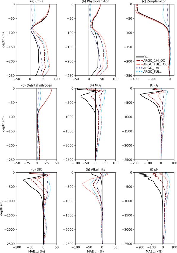
mation to that gained from the much denser ocean colour
observations, at least at the global scale. When only BGC-
Argo was assimilated, a small improvement at the surface of
7 % and 15 % was seen in ARGO_1/4 and ARGO_FULL,
respectively. Beneath the surface, at depths likely to see a
deep chlorophyll maximum, BGC-Argo had much greater
impact, with all four runs outperforming OC. ARGO_FULL
outperformed ARGO_1/4, demonstrating benefit from ex-
tra in situ observations. Combining BGC-Argo and ocean
colour gave better results at this depth in ARGO_1/4_OC
(which is the proposed observing system), but ARGO_FULL
and ARGO_FULL_OC performed similarly. Beneath the eu-
photic zone, where Chl a was near zero, the assimilation had
Figure 6. Time series of daily global RMSE for surface little impact. Positive values of MAEred_% were seen below
log10 (Chl a) between FREE and CCI ocean colour observations 250 m, but values of MAEred_abs (not shown) tended to zero
(black line) and between FREE and NATURE (red line) at CCI below about 220 m.
ocean colour observation locations. The results for phytoplankton biomass were very similar
to those for Chl a. For zooplankton biomass, which was not
directly updated by the assimilation, a large degradation in
ally appropriate levels of error with a complex biogeochemi- surface values was seen in all three runs assimilating ocean
cal model with globally uniform parameterisations could not colour data, with the impact reducing to near zero at around
be managed within the resources of the project. Furthermore, 100 m. A smaller degradation was seen in ARGO_FULL that
the similarity of Chl a between NATURE and FREE in some was reduced further in ARGO_1/4. Detrital nitrogen was im-
regions was due to the introduction of compensating errors proved in the upper 100 m in all runs, especially those assim-
in FREE rather than a lack of model error. This itself is a ilating ocean colour, with little absolute impact of the assim-
common feature of reanalyses, which can result in data as- ilation beneath that depth.
similation increasing overall error by correctly reducing one For NO3 and O2 , which were assimilated from the BGC-
of a set of compensating errors, as demonstrated by Ford and Argo floats, there was a clear improvement throughout the
Barciela (2017). For regions and variables for which the er- water column to 2500 m in ARGO_1/4 and ARGO_FULL,
rors between FREE and NATURE were too low, the poten- with greater improvement when more floats were assimi-
tial result may be to underestimate the impact of assimilating lated. Maximum MAEred_% was seen at 100–120 m of depth,
dense data, in this case ocean colour, and overestimate the with less of an impact at the surface, particularly for O2 . In
impact of assimilating sparse data, in this case BGC-Argo OC, NO3 and O2 were degraded in the upper 1000 m. Adding
(Halliwell et al., 2014). This should be borne in mind when BGC-Argo to ocean colour assimilation partially mitigated
drawing conclusions. this, with positive MAEred_% at some depths and negative
MAEred_% at others.
4.2 Assimilation runs With the carbon cycle, DIC, alkalinity, and pH were all de-
graded in OC. In ARGO_1/4 and ARGO_FULL, throughout
For each of the five assimilation runs, profiles of global most of the water column DIC was improved and alkalin-
MAEred_% over FREE for December 2009 are plotted in ity degraded, with an overall improvement in the assimilated
Fig. 7 for nine model variables. The results for MAEred_abs variable pH. Combining ocean colour and BGC-Argo assim-
are very similar to those for MAEred_% (not shown). For ilation gave mixed results, with a degradation in pH in the
Chl a (Fig. 7a), phytoplankton biomass (Fig. 7b), zooplank- surface layers but an improvement at depth.
ton biomass (Fig. 7c), and detrital nitrogen (Fig. 7d), which Spatial maps of surface MAEred_% over FREE for Decem-
only have significant concentrations in the euphotic zone, ber 2009 are plotted in Fig. 8 for the five assimilation runs
profiles are plotted for the upper 250 m. For NO3 (Fig. 7e), for Chl a, NO3 , O2 , pH, and pCO2 . In OC surface Chl a
O2 (Fig. 7f), DIC (Fig. 7g), alkalinity (Fig. 7h), and pH was almost universally improved (Fig. 8a), apart from a few
(Fig. 7i), profiles are plotted for the upper 2500 m. Recall small areas in the Atlantic, North Pacific, and Indian Ocean.
that Chl a, NO3 , O2 , and pH observations, assimilated in These correspond to areas where NATURE and FREE were
the BGC-Argo experiments, were produced for the upper almost identical, as seen in Fig. 3d, so the observation er-
2000 m. rors were larger than the model error. Very little difference
For Chl a, OC, ARGO_1/4_OC, and ARGO_FULL_OC was made by adding BGC-Argo to ocean colour assimila-
all had an MAEred_% value of 72 % at the surface. This sug- tion, while assimilating just BGC-Argo data gave mixed re-
gests that ocean colour was very successful at improving sur- sults for Chl a at the surface. In the Pacific Ocean, Chl a
face Chl a, while BGC-Argo was unable to add much infor- was slightly improved in ARGO_1/4 and further improved
https://doi.org/10.5194/bg-18-509-2021 Biogeosciences, 18, 509–534, 2021522 D. Ford: Assimilating synthetic Biogeochemical-Argo and ocean colour observations Figure 7. Profiles of global MAEred_% over FREE for December 2009. Note that axis scales differ between subplots. in ARGO_FULL, while in the Atlantic and Indian Ocean of the largest differences were seen between NATURE and a degradation was seen. This again corresponds to regions FREE (Fig. 3f). Adding BGC-Argo assimilation increased where there was little absolute difference between NATURE this improvement and started to reverse the degradation in and FREE (Fig. 3d). As such, MAEred_% is not the most in- other regions, particularly in ARGO_FULL_OC. Assimilat- formative metric in these regions, and it is more appropriate ing just BGC-Argo improved NO3 in most areas, with more to examine MAEred_abs . This is plotted for Chl a in Fig. 9, impact seen with more floats, but the results were patchy in which shows the absolute value of the degradation to be very places. small. The story for O2 (Fig. 8k–o) was very similar to that for Surface NO3 was degraded almost everywhere in OC NO3 but with a smaller degradation introduced by ocean (Fig. 8f), apart from the tropical Pacific, which is where some colour assimilation and a smaller improvement brought Biogeosciences, 18, 509–534, 2021 https://doi.org/10.5194/bg-18-509-2021
D. Ford: Assimilating synthetic Biogeochemical-Argo and ocean colour observations                                         523

Figure 8. Surface MAEred_% over FREE for Chl a, NO3 , O2 , pH, and pCO2 for December 2009.

Figure 9. Surface MAEred_abs over FREE for Chl a for December 2009.

https://doi.org/10.5194/bg-18-509-2021                                                       Biogeosciences, 18, 509–534, 2021
524 D. Ford: Assimilating synthetic Biogeochemical-Argo and ocean colour observations
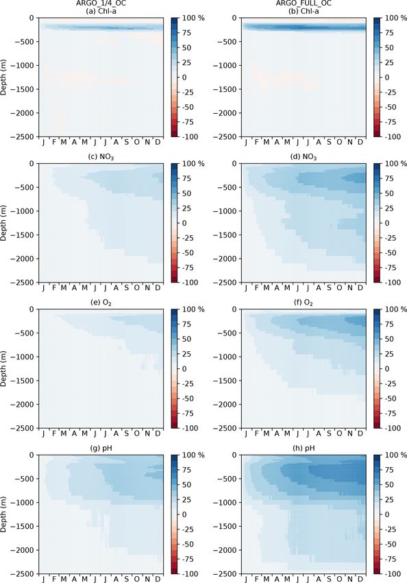
for each of the assimilated variables for ARGO_1/4_OC
and ARGO_FULL_OC in Fig. 11. For Chl a (Fig. 11a, b),
ARGO_1/4_OC and ARGO_FULL_OC both displayed a
very small degradation compared with OC in the surface lay-
ers throughout the year. This is consistent with the small
difference seen between the runs in the profiles in Fig. 7a.
Between about 80 and 300 m of depth, where deep chloro-
phyll maxima may be found, a strong positive impact was
found on Chl a, which was strongest in ARGO_FULL_OC.
In both runs this took a few weeks to spin up, then re-
mained reasonably consistent throughout the year. Beneath
about 300 m of depth, values of MAEred_% were near zero,
as Chl a was negligible. For NO3 , O2 , and pH, an almost
universal improvement was seen throughout the water col-
umn. For all three variables, values of MAEred_% were high-
est in the upper 1000 m, with a maximum at a similar depth
or slightly deeper than that for Chl a. MAEred_% was consis-
tently higher in ARGO_FULL_OC than in ARGO_1/4_OC,
again demonstrating a positive impact from having a greater
number of BGC-Argo floats. In both runs, MAEred_% in-
creased throughout the year, suggesting that the impact of
the assimilation was still spinning up, and the full potential
would not be realised until the system had been run for longer
than a year.
In Fig. 11, global MAEred_% is shown. As can be seen in
Fig. 10, the subsurface impact of the BGC-Argo assimilation
was not globally uniform, with a stronger impact typically
seen at low latitudes than at high latitudes. To demonstrate
this further, equivalent versions of Fig. 11 are shown for the
Figure 10. MAEred_% over OC for Chl a, NO3 , O2 , and pH for tropical Pacific in Fig. 12 and for the Southern Ocean in
December 2009 at 100 m of depth.
Fig. 13. In the tropical Pacific, the patterns for all the assim-
ilated variables were very similar to the global average but
with higher MAEred_% values, showing a stronger positive
about by BGC-Argo assimilation. For pH (Fig. 8p–t) and impact of the assimilation. This was especially large for Chl a
pCO2 (Fig. 8u–y), the patterns were also similar but with a between 80 and 300 m of depth and pH in the upper 1000 m.
greater degradation introduced by ocean colour assimilation MAEred_% values for Chl a were largely negative below
and a greater improvement brought about by BGC-Argo as- 300 m, but MAEred_abs values were near zero (not shown)
similation. Improvements to DIC and alkalinity when assim- due to Chl a concentrations being negligible. For NO3 , O2 ,
ilating pH should also help improve pCO2 , which was not and pH, the impact of the assimilation was still spinning
directly assimilated, though the details of the impact differ up after a year. In the Southern Ocean, MAEred_% values
between the two variables. were much lower, with an especially limited impact from the
Current state-of-the-art reanalyses typically assimilate BGC-Argo assimilation in ARGO_1/4_OC. MAEred_% was
ocean colour data (Fennel et al., 2019), so to demonstrate the typically largest for pH and lowest for Chl a. The impact
additional impact BGC-Argo might have in these systems, of the assimilation continued to increase with time, so it may
the remainder of this section focusses on MAEred_% over OC have just been taking longer to spin up than at lower latitudes.
rather than over FREE. Spatial plots of MAEred_% over OC Similar results were seen in the Arctic Ocean (not shown). In-
for December 2009 at 100 m of depth are shown in Fig. 10 for crements also spread further in tropical regions due to longer
the assimilated variables Chl a, NO3 , O2 , and pH. Clear ben- correlation length scales and faster propagation timescales.
efit was found for all variables, with greater improvements
than at the surface. The improvement was largest for pH and
smallest for Chl a, and in all cases a greater impact was seen 5 Summary and discussion
in ARGO_FULL_OC than ARGO_1/4_OC.
To investigate the impact of the BGC-Argo assimilation A set of observing system simulation experiments (OSSEs)
over the full year, a Hovmöller diagram (Hovmöller, 1949) was performed to explore the impact on global ocean bio-
of daily global MAEred_% over OC with depth is plotted geochemical reanalyses of assimilating currently available
Biogeosciences, 18, 509–534, 2021 https://doi.org/10.5194/bg-18-509-2021You can also read