Doris Breuer2 Electrical and seismological structure of the martian mantle and the detectability of impact-generated anomalies
←
→
Page content transcription
If your browser does not render page correctly, please read the page content below
Thomas Ruedas1,2

                                                                                                    Doris Breuer2

                                                  Electrical and seismological structure of the martian mantle and the
                                                               detectability of impact-generated anomalies

                                                                                                     final version

                                                                                                18 September 2020
arXiv:2003.06799v2 [astro-ph.EP] 6 Feb 2021

                                                                                                    published:
                                                                                            Icarus 358, 114176 (2021)

                                                                                      1
                                                                                          Museum für Naturkunde Berlin, Germany

                                                               2
                                                                   Institute of Planetary Research, German Aerospace Center (DLR), Berlin, Germany

                                              The version of record is available at http://dx.doi.org/10.1016/j.icarus.2020.114176.
                                              This author pre-print version is shared under the Creative Commons Attribution Non-Commercial No Derivatives License (CC BY-NC-ND
                                              4.0).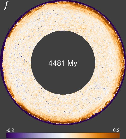
Electrical and seismological structure of the martian mantle and the
                 detectability of impact-generated anomalies
                                                         Thomas Ruedas∗
                                               Museum für Naturkunde Berlin, Germany
                            Institute of Planetary Research, German Aerospace Center (DLR), Berlin, Germany

                                                           Doris Breuer
                            Institute of Planetary Research, German Aerospace Center (DLR), Berlin, Germany

    Highlights

    • Geophysical subsurface impact signatures are detectable under favorable conditions.
    • A combination of several methods will be necessary for basin identification.
    • Electromagnetic methods are most promising for investigating water concentrations.
    • Signatures hold information about impact melt dynamics.

Mars, interior; Impact processes

                                                              Abstract
           We derive synthetic electrical conductivity, seismic velocity, and density distributions from the results of martian
       mantle convection models affected by basin-forming meteorite impacts. The electrical conductivity features an
       intermediate minimum in the strongly depleted topmost mantle, sandwiched between higher conductivities in the
       lower crust and a smooth increase toward almost constant high values at depths greater than 400 km. The bulk
       sound speed increases mostly smoothly throughout the mantle, with only one marked change at the appearance of
       β-olivine near 1100 km depth. An assessment of the detectability of the subsurface traces of an impact suggests that
       its signature would be visible in both observables at least if efficient melt extraction from the shock-molten target
       occurs, but it will not always be particularly conspicuous even for large basins; observations with extensive spatial
       and temporal coverage would improve their detectability. Electromagnetic sounding may offer another possibility to
       investigate the properties of the mantle, especially in regions of impact structures. In comparison with seismology
       and gravimetry, its application to the martian interior has received little consideration so far. Of particular interest
       is its potential for constraining the water content of the mantle. By comparing electromagnetic sounding data of
       an impact structure with model predictions, it might also be possible to answer the open question of the efficiency
       of extraction of impact-generated melt.

1      Introduction
The electrical, seismic, and density structures of the mantles of terrestrial planets reflect in multiple ways the physical
and chemical state and history of their interiors, but observations of any of them are only snapshots of the present
situation and lack the temporal dimension. By contrast, dynamical numerical models of mantle evolution provide
both spatial and temporal information and can therefore give insights into processes of whose products we can today
only observe the scrambled and diluted remains with often ambiguous signatures. Convection models per se do not
need information about seismic and electrical properties as input, and many of them use only some fairly simple
representation of the density, and so they are generally not suited for deriving the seismic or electrical structure.
Nonetheless, it is possible to integrate a more detailed description of the mantle’s minerals and their properties into
them and thus derive models of seismic and electrical structure from the same mineralogical model as the dynamical
evolution model.
    The prediction of seismic velocities and/or electrical conductivity from such convection models has already been
attempted in some previous studies of terrestrial mantle convection but to our knowledge not for other planets.
Goes et al. (2004) ran a suite of extended Boussinesq models of thermal convection that included phase transitions
and a depth dependence of some thermoelastic properties. The authors used some material parameters adjusted to
be compatible with the compilation of seismic property data that they then used to derive seismic velocities and
attenuation models from the dynamical models. However, they did not include compositional changes due to melting,
and the thermoelastic property framework was not internally self-consistent. Kreutzmann et al. (2004) and Ruedas
    ∗ Corresponding   author: T. Ruedas, Museum für Naturkunde Berlin, Germany (Thomas.Ruedas@mfn.berlin)

                                                                  2
(2006) used a similar type of convection models that did include melting and its effect on composition but derived
seismic velocity anomalies (rather than absolute velocities) and attenuation from empirical rock-physical relations.
They also calculated an electrical conductivity model based on limited experimental data for some minerals, whole
rock, and silicate melts, whereby the latter study also included the effect of water. Nakagawa et al. (2009) and Tirone
et al. (2012) were the first to combine dynamical convection models with internally self-consistent thermoelastic
models, which makes the calculation of density variations an integral part of the dynamic model, and used them
to predict seismic observables. However, both studies limited their application only to S-wave anomalies, although
P-wave distributions would have been a straightforward by-product of their models. In the present study, we combine
information from an internally consistent set of mineral end-member thermoelastic properties with an empirical model
of mantle petrology to calculate the material properties of the martian mantle and crust. These properties are
then used in both the dynamical model and the thermoelastic observables that yield a model of the density and
seismological structure of the silicate part of Mars. The same petrological model is also used for the derivation of
electrical conductivity distributions. As a major focus of this paper lies on processes in which an impact is large
enough to affect the mantle and to trigger a longer-term regional effect, the emphasis of our considerations lies on
large-scale effects on the mantle and crust rather than on local structure.
    Some of the oldest, largest, and in some cases most conspicuous features of the martian surface are basins formed
by large impacts. The largest of these basins, such as Utopia, Ares, or Acidalia, have diameters of more than 3000 km,
and the impacts thought to have produced them must have had substantial regional or even global effects on the
martian interior, because they have penetrated down to the sublithospheric mantle and exerted a direct influence on
convection and melting in the mantle (e.g., Reese et al., 2002, 2004; Watters et al., 2009; Roberts et al., 2009; Golabek
et al., 2011; Roberts and Arkani-Hamed, 2012; Ruedas and Breuer, 2017). Ruedas and Breuer (2017) showed that
the thermal and chemical anomaly produced by the impact and concomitant melting is deformed and successively
obliterated by the vigorous convective mantle currents it has triggered. However, under assumptions that increase
the viscosity of the mantle, e.g., a low water content, remnants of the chemical anomaly can survive to the present.
These anomalies should in principle also be detectable by geophysical methods, but such methods have so far been
restricted to orbiting spacecraft, most importantly gravity and magnetic observations. There is more than one possible
interpretation of such potential field signatures, however, and further assumptions have to be made to constrain them.
Observations of Mars’ magnetic field provide information mostly on crustal magnetization, and processes like shock or
thermal demagnetization or re-magnetization of target materials in the presence of an external field (e.g., Lillis et al.,
2013) make them more difficult to interpret.
    In this paper, we revisit and supplement some of the models from Ruedas and Breuer (2017), which tracked the
evolution of a Mars-like planet that experienced a single basin-forming impact, and calculate the resulting anomalies of
some geophysical observables. Our earlier study was mostly concerned with various aspects of the dynamical evolution
and its relations with heat flow as well as with gravity. The focus in the present paper lies mostly on assessing
the necessity of more ground-based geophysical studies, i.e., on methods that can not or only with limitations be
applied from orbiters but potentially deliver less ambiguous results than gravity or magnetic measurements on both
global structure and regional features such as impact sites. These methods are especially electromagnetic and seismic
soundings. The latter is being pioneered now by the InSight mission (e.g., Lognonné et al., 2019; Panning et al., 2017),
but the former has received little attention so far. There have been some electromagnetic soundings of the Earth’s
mantle using magnetometer data of orbiting satellites (e.g., Constable and Constable, 2004), but the only evaluation
of measurements at Mars known to us is an attempt by Civet and Tarits (2014), who derived a radial conductivity
profile of the martian mantle from Mars Global Surveyor (MGS) magnetometer data. It may be possible to derive
usable data from measurements of the magnetometer on the InSight lander as a by-product of that mission (e.g., Chi
et al., 2019; Russell et al., 2019; Mittelholz et al., 2020; Yu et al., 2020), although those data are not expected to be
of the highest quality and will be affected by noise from the lander. Nonetheless both methods have the potential to
elucidate the large-scale basic structure of the martian mantle and constrain dynamically relevant properties such as
the crustal thickness or the position and width of phase boundaries.
    The motivation for applying electromagnetic and seismic methods to impact structures in addition to the data
already available is twofold. First, there are cases of basins with diameters above 1000 km, especially among very
early structures, whose identity as being impact-generated is not firmly established. For instance, the impact origin
of Chryse Planitia, which has a diameter of 1725 km and an age similar to the aforementioned three largest basins,
has long been disputed and is still being studied (e.g., Pan et al., 2019). The list of impact basins by Frey (2008),
which has been used in several dynamical studies, contains 20 entries, and follow-up work by Frey and Mannoia
(2014) ramps this count up to as many as 31 candidate structures, which are rated according to criteria such as
topographic or crustal thickness expression. On the other hand, Bottke and Andrews-Hanna (2017) argued that the
observation that the dichotomy boundary is crossed by only one basin of this magnitude (Isidis) makes a number of
more than 12 basin-forming impacts between the dichotomy-forming event and the final cadence defined by Hellas,
Utopia, Isidis, and Argyre highly unlikely from a statistical point of view. If additional means such as geophysical
signatures originating in the deeper interior are available to confirm or dismiss candidate impact structures, the impact
count and in consequence the influence of impacts on martian evolution could be better assessed.
    The second incentive is to help quantify how impact-generated melt is extracted from its source after the impact.
The extreme heating by the shock is expected to melt a part of the target, and melting efficiency increases if the target
was already close to the solidus temperature before the impact, as would be the case for a very large event that reaches

                                                            3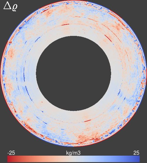
into the mantle. Factors such as the high permeability of the partially molten target or the dynamics of post-impact
uplift can be imagined to promote massive eruption of impact melts. In this case, the residue would be very strongly
depleted in fusible components and be even more stripped of incompatible trace components than the background
mantle, and a thick post-impact crust with an abnormally low concentration in heat-producing elements and volatiles
is expected to form. On the other hand, it is also conceivable that at least a part of the melt remains trapped in
the interior and recrystallizes, because the lifetime of potential melt migration pathways after the impact is too short
or the prevailing stress field is unfavorable to melt extraction. As a consequence, the target mantle would be much
less or not at all depleted, and the pre-impact crust blasted off by the impact would not or only partly be replaced
by erupting post-impact melt. This would potentially explain the reduced crustal thicknesses inferred from gravity
for various large basins such as Hellas on Mars (e.g., Neumann et al., 2004) or the South Pole–Aitken basin on the
Moon (e.g., Wieczorek et al., 2013). The presence or absence of geophysical signatures that depend on the efficiency of
impact melt extraction in confirmed impact structures could therefore put constraints on models of melt production
during the impact process. Their dynamics are only beginning to be investigated in detail (e.g., Manske et al., 2019,
2021), and they could also improve the treatment of impacts in evolutionary geodynamical models. The fate of this
melt is likely to have implications for the local dynamics of the mantle and its melt productivity in the post-impact
phase and for the resulting geochemical variability. In the literature, scenarios ranging from no extraction (Padovan
et al., 2017) to substantial extraction (Golabek et al., 2011; Ruedas and Breuer, 2017) have been considered. By using
models from the latter study as the starting point for this investigation, we assume a scenario that would maximize
the expected effects. However, in order to assess the importance of extraction, we supplemented those models with
some additional ones in which impact melt extraction was suppressed.

2    Method
The models of Ruedas and Breuer (2017) were fully dynamical mantle convection calculations on a two-dimensional
spherical annulus grid with pressure-, temperature-, and composition-dependent viscosity and internal and basal
heating, carried out with a modified version of StagYY (Tackley, 1996, 2008; Hernlund and Tackley, 2008) in the
anelastic, compressible approximation; a list of specific model parameters and the characteristics of the impact basins
is provided in Table 1. They were coupled with a detailed mineral physics model of martian mineralogy after Bertka
and Fei (1997) based on the bulk silicate Mars composition from Wänke and Dreibus (1994). That model combines
thermoelastic data for the mineral end-members with experiment-based parameterizations of the phase diagram and
petrology of the martian mantle and empirical formulas for various major- and minor-element abundances in the
mineral solid solutions, in particular for Mg–Fe partitioning. The partitioning formulas for the individual mineral
phases were taken from the literature or constructed from available published experimental data. They describe the
dependencies of the partitioning coefficients on pressure, temperature, and composition to the (quite variable) extent
permitted by the data; full details can be found in the Supporting Information of Ruedas and Breuer (2017). The
model therefore reproduces closely the martian mantle petrology for the chosen bulk silicate composition and ensures
that the same physical and chemical properties that controlled the dynamical evolution of those convection models
are now also used for the derivation of seismic velocities and electrical conductivity. As we do not have a similar
representation for crustal material, the crust was assigned a homogeneous MORB-like mineralogy consisting mostly
of clinopyroxene and plagioclase (e.g., Litasov and Ohtani, 2007), although its water content is derived from the
dynamical model. Compositional variability such as lithological inhomogeneities or depletion due to melting is tracked
with tracer particles. The melt dynamics is simplified by extracting segregating melt instantaneously and adding it to
the top of the corresponding column of the numerical grid.
    Melting was included in the dynamical models as a cause of chemical variations that affected the dynamical behavior
and also left its signature in geophysical observables, even though no melt is found to exist in the martian interior
today on a global scale. This is consistent with other models of the thermal evolution of Mars (e.g., Plesa et al.,
2018), which also find the conditions for melting to be fulfilled at most at some isolated local sites in modern Mars.
The key compositional features considered in connection with melting were the iron, radioactive element, and water
concentrations. The latter was varied between the nominal bulk silicate Mars value from Wänke and Dreibus (1994)
of 36 ppm and its two- and fourfold (72 and 144 ppm) with the purpose of probing its effect on convective vigor.
    An impact is imposed as an instantaneous thermal anomaly with a shape determined from simple scaling laws
and a temperature distribution derived from an impedance match calculation and empirical fits to the shock pressure
decay from numerical impact simulations (Reese et al., 2002; Watters et al., 2009; Ruedas, 2017). The impactor strikes
at 4 Ga, which is 400 My after the start of the modeled evolution, and is specified as having a magnitude that would
result in a basin of the size of either Huygens, Isidis, or Utopia. Each of them stands as a representative example of a
size class: the Huygens impact produced a crater a few hundred kilometers wide and affected mostly the lithosphere;
the Isidis impact formed a basin with a diameter of ∼1000 km and had effects that reached below the lithosphere; the
Utopia impact resulted in a basin of almost 3400 km and melted even parts of the mantle below the maximum depth
of regular melting at its time of formation (see Table 1). The site of the impact is chosen such that a coincidence with
a hot upwelling or a cold downwelling is avoided as far as possible in an attempt to produce an effect representative
for the mean thermal structure of the target, as local variations would modify the thermal effects of shock-heating;
therefore, the impacts are at different locations in models with different water contents.

                                                           4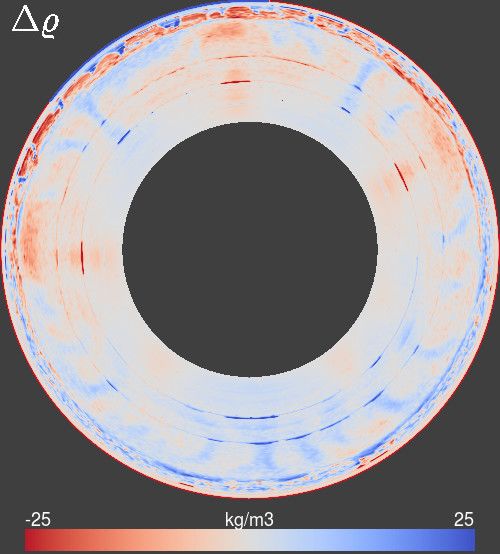
Almost all of the melt produced by it and in its aftermath is extracted to build the crust and is assumed to fill
the near-surface pore space that is imposed at the top of the crust, whereby it is assumed to lose heat very efficiently
and thus attain surface temperature immediately, i.e., to crystallize within a single timestep, which is typically on
the order of 10 ky. According to independent estimates (e.g., Reese and Solomatov, 2006; Reese et al., 2007), the
crystallization of the impact-generated melt pond happens to occur on similar or even shorter timescales. More
importantly, the crust forming by the crystallization of the post-impact melt pool will have a very low porosity. In
this paper, we refer to these processes, which result in the impact basin being turned into a low-porosity anomaly,
as “porosity deletion” or similar terms. As the model algorithm cannot handle a completely liquid body inside the
essentially solid planet, a maximum melting degree that can be reached has to be set and is fixed here at 60%, which
corresponds to the absence of practically all fusible components (pyroxenes, most of the Al-bearing phases and fayalite
fraction in olivine). Such upper limits to the contribution of melts to crust formation have also been defined in other
studies of impact–convection interactions (e.g., Golabek et al., 2011). They effectively entail an upper bound on the
thickness of the post-impact melt sheet and crust and imply immediate in-situ recrystallization in, or inefficient melt
extraction from, the central parts of the shocked source region to the surface for some part of the target. We expect
that without this restriction, the impact melt would be even more mobile, and the potentially extracted melt volume
and the magma pond it forms would be even larger and have a more strongly ultramafic composition. The observed
seismic and electric anomalies in the mantle source regions of these melts should also be more pronounced in this
case. When the magma pond crystallizes and differentiates, melts from source regions with different melting degrees
are presumably mixed, and the mineralogy that results after crystallization represents an average composition of all
melts, such that the geochemical signal from the most extreme melting is muted. Some implications of the efficiency
of melt extraction for the formation of post-impact crust will be discussed in Sect. 4.3.
    We use a pressure-dependent porosity profile to describe the decay of porosity with depth in the megaregolith and
its effects on density and thermal conductivity. The result of porosity deletion by impact melts is then the erasure of
that porosity; we do not model the temporal changes in porosity due to impacts of smaller sizes throughout the history
of the planet, and hence, porosity once destroyed by melt is not restored. By doing so, we ignore the new formation
of regolith by the constant flux of smaller meteorites, but on the length-scale of megaregolith that reaches to several
kilometers depth, this assumption should be acceptable, because at this stage in planetary evolution no substantial new
formation of megaregolith is expected, and it is only this large length-scale that can be resolved at least rudimentarily
in our global model at all. Recent analyses of the shallow density structure in and around large lunar impact craters
determined that the porosity in many of them is indeed substantially reduced, probably as a consequence of impact
melt filling the pore space (Wahl and Oberst, 2019; Wahl et al., 2020, and D. Wahl, pers. comm.). This simplified
treatment facilitates the formation of crustal density anomalies and has implications for the geophysical signatures
of impacts, as will be discussed below. Furthermore, variants of the models with the lowest water content were run
in which the extraction of melt generated directly by the impact was suppressed. As a consequence, that melt was
assumed to recrystallize in situ in those cases, and magma-flooding of the crater and the concomitant deletion of
porosity did not occur. Melt produced by magmatism in the millions of years following the impact is extracted in both
scenarios. In this paper, our attention will mostly be directed at the models with impact melt extraction, however.
Finally, an additional impact-free model was also included for each of the three initial water concentrations considered;
these models were called “reference models” in Ruedas and Breuer (2017).
    The density % and other thermoelastic properties of the martian crust and mantle are determined from thermo-
dynamic data for the mineral end-members, which are assumed to form the constituent minerals of the rock as ideal
solid solutions. The thermoelastic bulk rock properties are determined in three steps: first, the end-member properties
at the desired pressure and temperature are calculated; second, the properties of the individual mineral phases are
calculated from them assuming ideal solid solution; third, the bulk rock properties are computed as those of a mixture
of the individual phases. In particular, the bulk sound speed vB is calculated as the Voigt–Reuss–Hill average of the
mineral assemblage (Mavko et al., 1998) from the densities and the adiabatic bulk moduli KS of the mineral phases,
because our database of thermoelastic properties does not include the shear modulus information necessary to calcu-
late tighter bounds, and theoretical estimates of the shear modulus did not generally achieve an accuracy that would
justify their use. The calculation is described in more detail in the Supplementary Material of Ruedas and Breuer
(2017).
    The electrical conductivity σ is determined in two stages from available experimental data on various minerals that
are usually not end-members. The conductivity of individual minerals results from the diffusive movement of charge
carriers, i.e., of ions (protons or other species) or small polarons (electron–hole pairs) that move through the lattice
or along grain boundaries. It can therefore be described by a generalized Arrhenius-type expression of the form
                                                                  1                  !
                                               qi       Ei − αi Ci3 + p(Vi − βi Ci )
                                      σ = σ0i Ci exp −                                 ,                              (1)
                                                                    RT

where p and T are pressure and temperature, Ci is the concentration of the ith charge carrier, Ei and Vi are the
activation energy and volume, σ0i , qi , αi , and βi are material constants, and R is the molar gas constant; this form
unifies various extensions of the classic Arrhenius law that are found in the literature in order to include compositional
effects. There are in general several different types of charge carriers in a mineral phase, whose contributions to its
total conductivity are additive. Of particular interest are the small polarons that arise from surplus charges introduced

                                                            5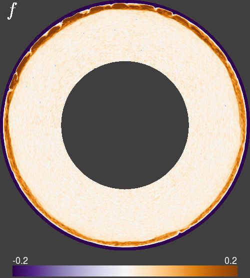
Table 1: General model parameters.
Planetary radius, RP                                  3389.5 km                     Archinal et al. (2011)
Total planetary mass, M                            6.4185 · 1023 kg                 Konopliv et al. (2011); Jacobson (2010)
Surface temperature                                     218 K                       Catling (2015)
Mantle
Mantle thickness, zm                                 1659.5 km                      Rivoldini et al. (2011)
Initial potential temperature, Tpot                    1700 K
Initial core superheating                               150 K
Surface porosity, ϕsurf                                   0.2                       Clifford (1993)
Melt extraction threshold, ϕr                           0.007                       after Faul (2001)
Grain size, d                                           1 cm                        Hirth and Kohlstedt (2003)
Bulk silicate Mars Mg#                                   0.75                       Wänke and Dreibus (1994)
Present-day K content                                 305 ppm                       Wänke and Dreibus (1994)
Present-day Th content                                 56 ppb                       Wänke and Dreibus (1994)
Present-day U content                                  16 ppb                       Wänke and Dreibus (1994)
Initial bulk water content                       36, 72, 144 ppm                    after Wänke and Dreibus (1994)
Core (average material properties)
Core radius                                           1730 km                       Rivoldini et al. (2011)
Sulfur content                                        16 wt.%                       Rivoldini et al. (2011)
Thermal expansivity*,† , αc                     3.5–4.3 · 10−5 1/K
Isobaric specific heat, cpc                        750 J/(kg K)                     after Stacey and Davis (2008)
                       *
Thermal conductivity , kc                      23.5–25.1 W/(m K)
Model impact/crater parameters        Huygens         Isidis        Utopia
Final crater diameter, Df            467.25 km      1352 km        3380 km          Roberts et al. (2009); Frey (2008)
Age                                   3.98 Gy    3.81–3.96 Gy 3.8–4.111 Gy          Werner (2008)
                    *
Impactor diameter , Dimp              70.6 km       243.5 km       699.2 km
Depth of isobaric core* , zic         21.5 km        74.1 km       212.9 km
Radius of isobaric core* , ric        19.5 km        67.1 km       192.6 km
  *                         †
    Calculated during run. Varies with time.

by Fe3+ and cause a dependence on iron content, and the protons that are formed by the dissociation of trace water
and strongly enhance the conductivity especially at temperatures that would be expected in the lithosphere. Our
models do not indicate the presence of significant amounts of melt on a large scale in the present-day martian interior,
especially not beneath large old impact basins. As we have no reliable constraints on the abundance of ice or water
in the near-surface regions either, we limit ourselves to the conduction in nominally anhydrous minerals. Hence we
first calculate the conductivities of the individual mineral phases using the parameters compiled in Table 3 and taking
into account variations of their iron and water contents due to past melting processes and the partitioning of water
between the mineral phases according to empirical partition coefficients, as far as such variations are experimentally
constrained (e.g., Aubaud et al., 2008; Bell and Rossman, 1992; Grant et al., 2007; Hauri et al., 2006; Hirschmann
et al., 2009; Inoue et al., 2010; Novella et al., 2014; O’Leary et al., 2010; Tenner et al., 2009). In the second step, we
compute the bulk conductivity of the rock as the self-consistent effective medium conductivity σEM given implicitly
by
                                                         N
                                                        X      σi − σEM
                                                    0=      xi                                                          (2)
                                                        i=1
                                                               σi + 2σEM

for a composite of minerals with total conductivities σi and volume fractions xi (cf. Bruggeman, 1935; Landauer,
1952; Berryman, 1995). The porosity of near-surface rock decays with depth due to self-compaction under overburden
pressure, which is implemented as a simple empirical exponential function and also correspondingly accounted for in
the calculation of %, vB , and σ.

3     Results
3.1    Dynamical evolution and global features of observables
All models start from an initial state derived from an adiabatic areotherm modified by melting that produced a
primordial crust and an initial random depletion of the entire mantle. The models go through an early stage of very
vigorous convection characterized by quite irregular and rapidly changing flow patterns that lasts several hundreds of
millions of years before entering a calmer and more orderly regime in which about half a dozen large and approximately
equally spaced mantle plumes emerges from the core–mantle boundary (CMB). Melting and crust formation, which
initially occurred globally throughout the outermost parts of the mantle, continue on an ever decreasing scale for a
few hundreds of millions of years before ceasing for good, with the exception of a few very minor and local eruptions.

                                                            6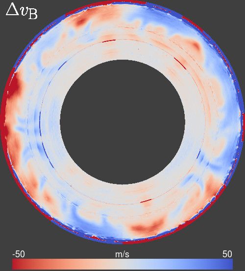
0

          200                                                                                                                                         DWAK
                                                                                                                                                      ZGDW
                     a)                                                                                              c)                                                        e)
          400

          600

                                                                                                                             opx-out
 z (km)

          800

                                                                                                                             rw-in
      1000
                                                                                                                             wd-in/ol+rw-out
                                                                                                                             rw-in
      1200
                     36 ppm
                     72 ppm                                                                                                  wd-out
      1400          144 ppm                                                                 Bertka & Fei                                                                   CT, preferred
                  dry solidus                                                       Smrekar et al., DWAK                     cpx-out                                       CT, unconstr.
                                                                           b)       Smrekar et al., ZGDW                                                    d)               CT bounds
                                                                                                                                                                                VV, EM
      1600                                                                                                                                                                       VV, HS

            250     500   750 1000 1250 1500 1750   -0.05   0       0.05   0.1   3000   3200   3400 3600      3800    4000    5        5.5      6     6.5        7   7.5   10-6 10-5 10-4 10-3 10-2 10-1 100 101 102
                               T (K)                            f                                 ρ (kg/m3)                                    vB (km/s)                                   σ (S/m)

Figure 1: Synthetic present-day depth profiles of temperature (a), depletion (b), density (c), bulk sound speed (d),
and electrical conductivity (e) of the crust and mantle of the impact-free models with different initial water contents
(solid colored curves). The temperature plot also includes the solidus of dry martian peridotite (Ruedas and Breuer,
2017, App. A) (dash-dotted gray curve); at the actual low water contents in the model, the solidus depression would
hardly be visible in this plot. Panel (b) also indicates the approximate depth intervals of the crust, the (thermal)
lithosphere, and the interval in which regular melting occurred in the ancient past; the approximate position of the
crust–mantle boundary is drawn as a dotted line. The gray data points in the density plot (c) are experimentally
determined values for a similar composition as assumed by us, taken from Bertka and Fei (1998) and rescaled to the
pressure–depth relation of our models; the gray curves in (c) and (d) are two of the 1D profiles for a composition based
on Wänke and Dreibus (1994) defined as Mars reference models by Smrekar et al. (2019). The gray curves in the
conductivity plot (e) are preferred inversion results and the bounds on the conductivity from Mars Global Surveyor
magnetometer data from Civet and Tarits (2014) (labeled CT) and the theoretical mineral-physics based models by
Verhoeven and Vacher (2016) (labeled VV) using the effective-medium value as in our model (EM) or the mean of the
Hashin–Shtrikman bounds (HS) (Hashin and Shtrikman, 1962); the data from Civet and Tarits (2014) are insensitive
toward structure at depths of more than 1300 km. The depths of several phase changes have been marked in (d) to
facilitate the correlation with discontinuities in the profiles. The full set of whole-mantle depth profiles for models
with and without impacts is available as part of the Supporting Material, Figs. S6 and S8.

As a consequence of melting, the mantle becomes depleted in iron oxide and, much more strongly, in the radioactive
elements and in water, which are very incompatible and thus become concentrated in the crust that is formed by
the extracted melt. 10% of the water in the melt extracted from the mantle is set to be lost permanently to the
atmosphere, assuming that volcanic activity on Mars is predominantly intrusive (e.g., Black and Manga, 2016). In
the present-day mantle, the former regular melting region is preserved as a depleted shell in the outermost part of the
mantle that has become immersed into the outer thermal boundary layer.
    Fig. 1 shows the calculated horizontally averaged present-day depth profiles of temperature, depletion due to
melting, density, bulk sound speed, and electrical conductivity, respectively, for the three impact-free models. For
comparison, independent observational and modeling data are also shown. Density data for a compositional model
based on Wänke and Dreibus (1994) (Fig. 1c) have been produced from experiments (Bertka and Fei, 1997, 1998)
or, along with seismic velocity predictions (Fig. 1d), theoretically (compiled by Smrekar et al., 2019). The electrical
conductivity (Fig. 1e) has been derived from orbiter magnetometer measurements by Civet and Tarits (2014) and
calculated theoretically for a Wänke–Dreibus model and various laboratory measurements by Verhoeven and Vacher
(2016). In spite of the different initial bulk water compositions of the models, the profiles are all very similar, because
most of the water is partitioned into the crust or lost by outgassing as a consequence of the chosen initial conditions
and the melting processes in the uppermost mantle early in the evolution, leaving behind a mantle with at most a few
tens of ppm of water even in the most water-rich model after 4.4 Gy (cf. Ruedas and Breuer, 2017). The temperature
profiles (Fig. 1a) show that the average temperatures are far below the mantle solidus, which makes it safe for us
not to consider the influence of melt on the observables. The depletion (f ) profiles (Fig. 1b) show that the strongly
depleted layer formed by early regular global melting beneath the young lithosphere is now firmly integrated into the
lithosphere; the steep shift to negative f marks the boundary between crust and mantle.
    Similar step-like changes can be seen in the profiles of % and vB ; the variations within the crust are mostly due
to the closure of pore space with depth and the steep temperature gradient. Smaller changes of %(z) and vB (z) can
be seen at different depths throughout the mantle and are due to the transformations of olivine to its higher-pressure
polymorphs and of the pyroxenes and garnet to majorite; the approximate positions of the transformations are also
visible as strong but very thin anomalies at the corresponding depths in Fig. 2, because the Clapeyron slopes of the
transitions cause variations in their depth according to the local temperature. The olivine transformations have a
more complex structure than in the Earth’s transition zone because of an additional appearance of the γ phase in the
more iron-rich martian mantle, but they are also broader due to the higher Fe content and the shallower lithostatic

                                                                                                 7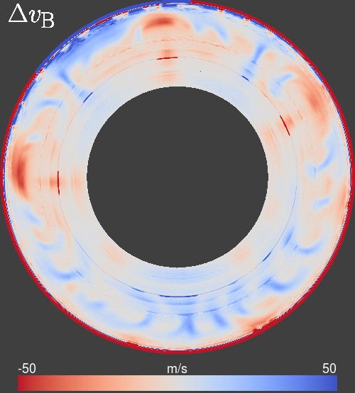
gradient (cf. Katsura and Ito, 1989; Katsura et al., 2004; Ruedas et al., 2013) and will therefore not cause reflections
that are as sharp as in the Earth.
   The only instance where a clear difference between the models with different water contents can be observed is the
lower crust and the uppermost mantle of the electrical conductivity profiles: especially in the lower crust, σ(z) differs
by up to a factor of 10 as a consequence of the different amounts of water that could be extracted from the mantle
source early in the planet’s history.

3.2    Features related to individual impacts
In models with an impact, the thermal anomaly triggers a pulse of strong, localized melting, which reinvigorates
mantle convection on a local or regional scale, depending on the size of the impact and the depth of penetration into
the sublithospheric mantle. In the models from Ruedas and Breuer (2017), in which the impact melt is extracted
and forms some sort of crust within the crater, the excessive production of melt also produces a strong compositional
anomaly with extreme depletion in incompatible components in the mantle. The thermal and compositional anomaly
rises and spreads beneath the lithospheric lid. While the thermal pulse diffuses away with time, the compositional
anomaly may persist if it is embedded quickly enough in the growing thermal boundary layer, which is relatively stable
due to its high viscosity; this occurs more easily in models with a low water content, because they have generally higher
viscosities and convect less vigorously. The final state of this process is shown in Fig. 2 (top row) and in Figs. S2–S5;
in the compositional field f , where depleted material is visible as regions with a brown hue, the remnants of the
impact appear as a dark brown area around the former impact site in the upper part of the cross-section that merges
gradually into the undisturbed depleted layer caused by regular melting.
    In the additional new models of this study, in which impact melt extraction is suppressed, the immediate in
situ recrystallization of the impact melt precludes the formation of a similarly strong compositional anomaly, but
nonetheless the mantle has been heated up to its solidus in the shocked region. The resulting substantial thermal
anomaly still triggers a strong local convective pulse in the aftermath of the impact that undergoes decompression
melting to some extent (e.g., Edwards et al., 2014) and thus results in the formation of post-impact crust and a
compositional anomaly. The latter is weaker than in the cases with extraction and does not spread as far; in terms of
global dynamic measures that quantify the vigor of convection such as the root-mean-square velocity of the convecting
mantle, the spike-like signature of the impact in models with retained impact melt lies between those with extracted
impact melt and models in which all compositional effects were ignored (Ruedas and Breuer, 2017). In contrast to
the models with extraction, whose final state features an anomaly characterized by extreme depletion, the mantle
beneath the basin in models with impact melt retention tends to show no or only slightly stronger depletion than the
reference toward the fringes and less depleted material toward the center, which has been drawn into that region by
the upwelling thermal anomaly (red and orange curves in Fig. 3b,g; also see the f plots in Fig. S9 of the supplementary
material). The final anomalies in all models are therefore generally broad, flat structures in the uppermost part of the
mantle. Significant differences between the models occur only in the uppermost ∼500 km, and so we focus on this depth
interval (Fig. 3). In both model variants, we make the assumption that the ejecta that end up within the final crater
and the crustal material between the rims of the transient and the final crater form a compositionally homogeneous
post-impact crust of constant thickness covering the entire area of the final crater that is emplaced immediately after
the impact (computationally speaking, in the same timestep as the impact itself, i.e., within a time span of ∼6000
to 18 000 years). A more refined representation is not possible due to the lack of a sufficiently simple mechanical
model and the limited resolution, nor is it necessary, because small-scale features within the crust are not expected
to influence the larger-scale effects on the underlying mantle significantly. As a result, we find no major differences in
the post-impact crustal thickness in the basins, as far as can be resolved by the vertical grid point spacing of ∼13 km.
    The Huygens impact is the smallest of the three events and barely reaches into the mantle; it is probably a good
example for the numerous minor impact basins. It causes a short-lived local disturbance in the uppermost mantle but
does not extend the range of melt production to depths greater than those affected by regular melting. Dynamically,
its principal effect is to trigger a small upwelling in the lithosphere and in the regular melting zone beneath it. As it
spreads beneath the lithosphere and disturbs its structure, it pushes some of the depleted mantle of the melting zone
away and sucks in more fertile material from below, but at this time the temperatures are already too low to let it
melt. As a result, the mantle anomaly is strongly depleted at the top but shows a decrease in f toward background
or even lower values further down, i.e., a blob of unusually fertile mantle sits in its lower part beneath the impact
site and becomes frozen in, because the thermal anomaly from the impact dissipates quickly; this blob tends to be
better preserved in models with lower water content (cf. Fig. S2). It has a higher density, mostly as a consequence of
its higher iron content. In the upper part, the densities and electrical conductivities are lower but seismic velocities
tend to be higher, although the spatial correlation is less sharp, and the deviation affects a larger region. The crust
is marked by a pronounced high-density, high-velocity, low-conductivity anomaly at depths shallower than ∼100 km.
The effects on density and velocity can be explained by porosity deletion by impact and post-impact melt, whereas
the effect on the conductivity seems to be dominated by its temperature dependence: the crust is abnormally cool,
mostly because the erupted impact melt is more depleted in radioactive heat sources, such that the crust formed from
it has a lower internal heating rate.
    While the character of the crustal anomaly is a constant of all models with impacts and impact melt extraction,
the character of the mantle anomaly is different in the Isidis-sized and the Utopia-sized events, which are substantially

                                                            8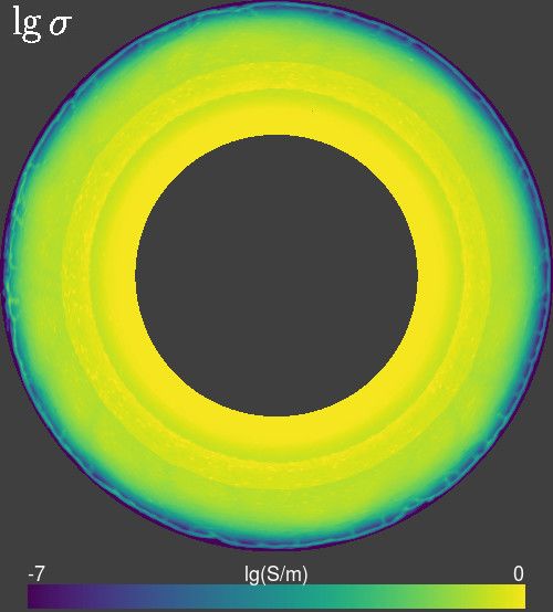
* *
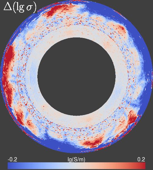
Figure 2: From left to right, top to bottom: Present-day temperature T , composition/depletion f , density anomaly
∆%, bulk sound speed anomaly ∆vB , and the decadic logarithm of the electrical conductivity σ and the corresponding
anomaly, for the Utopia-size impact in a model with 36 ppm initial bulk water. The approximate position of the center
of the isobaric core and of the outline of the original chemical anomaly are marked with an asterisk and a dashed
contour in the T and f panels. Except for T , the colorbars have been clipped for clarity. Cross-sections of the T
and f field at the time of impact and of all fields at the final state are provided for all models in the Supplementary
Material, Figs. S1–S5.
9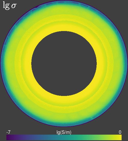
0

                                                                    Huygens

      100

      200
 z (km)

                  a)

      300

                        36 ppm
      400     36 ppm, no extr.
                       144 ppm
                                                                             b)       c)                              d)                                       e)
                   dry solidus
      500
        0

                                                                    Utopia

      100

      200
 z (km)

      300

      400

                  f)                                                         g)       h)                              i)                                       j)

      500

          200 400 600 800 1000 1200 1400 1600 -0.05 0 0.05 0.1 0.15 0.2 0.25 0.3   3420 3440 3460 3480 3500 3520   5.75 5.8 5.85 5.9 5.95   6   6.05 10-7   10-6    10-5   10-4 10-3   10-2   10-1
                         T (K)                                f                              ρ (kg/m3)                         vB (km/s)                                   σ (S/m)

Figure 3: Depth profiles of temperature (a, f), depletion (b, g), density (c, h), bulk sound speed (d, i), and electrical
conductivity (e, j) in the upper 500 km of the models with Huygens-size (upper row) and Utopia-size (lower row)
impacts. The solid lines are profiles of horizontal averages of the mantle volumes beneath the impact basin, the
dashed lines are global horizontal averages. Different colors indicate the different initial water contents of the models
(in ppm) and whether impact melt is extracted or not. The full set of profiles, including profiles at the basin centers
and the data for models with 72 ppm initial water, is available as part of the Supporting Material, Figs. S7 and S9.

                                                                                           10
larger and clearly affect the sublithospheric mantle. The shock-heated region is large enough to reach beyond the
lower margin of the regular melting zone and thus produces an extra volume of depleted mantle that is drawn in
by the impact-generated upwelling. As this depleted material has a lower density due to its lower iron content, the
corresponding mantle anomaly has a density deficit, contrary to the lower part of the Huygens-sized anomaly. The
seismic and conductivity anomalies are somewhat ambiguous with both positive and negative regions, but the positive
parts dominate again in the seismic velocities and the negative parts in the conductivities. The anomalies are usually
strongest beneath the point of impact and become weaker with distance from that axis, but by and large, depth
profiles of the anomaly horizontally averaged over the angular extent of the corresponding impact basin share many
features of the corresponding central profiles and tend to appear as somewhat muted and smoothed versions of them
(cf. Figs. S6–S9).
3.3 General impact-related features
3.3.1 Electrical conductivity
The electrical conductivity is sensitive to the changes in water and iron contents induced by melting and displays
contrasts of more than an order of magnitude between anomaly and reference in some cases (Fig. 3, rightmost column).
While all profiles are fairly similar in the deeper mantle, because even in the most water-rich models the mantle has
retained only a few tens of ppm water at most, the impact-generated anomaly is marked by a stronger conductivity
minimum than parts of the mantle that have only experienced regular melting. Given the generally low water content
of the mantle in all models, these contrasts are mostly due to stronger depletion in iron and the smaller fraction of
surviving pyroxene in the impact anomaly, where much higher melting degrees had been reached. The conductivity also
reveals more physical structure within the crust than the other methods considered: while they are mostly sensitive to
the porosity, σ(z) bears the mark of further influences and is therefore more variable between models. Compared to the
mantle, the crust is characterized by a marked increase of the conductivity across the compositional boundary between
the two, which is due to the mineralogy and the higher iron and water contents in the crust (Mg# ≈ 0.47 and H2 O
on the order of several hundred to a few thousand ppm). In particular the crustal water concentrations, which vary
between models according to the initial water contents, result in visible conductivity differences between the models;
these systematic differences with water content are most clearly expressed in the global average profiles, whereas
the profiles at the basin center may be influenced by local conditions. On the other hand, the strong temperature
dependence of σ reflects the slightly lower temperatures in the basin crust and comes to dominate at shallower depth
in combination with the increasing porosity.
3.3.2 Seismic velocities and density
In contrast to the electrical anomalies, the bulk sound speed and the density anomalies in the mantle are fairly small.
The vB anomalies are mostly positive and reach the largest values of up to 100 m/s in the uppermost mantle but
drop to generally less than 50 m/s beyond 150 km depth; beneath the Huygens basin, the anomalies are generally a
bit weaker due to the lesser size of the impact. The crust in the basin is always seismically faster in the models with
impact melt extraction because of the closure of pore space (Fig. 3). In terms of seismic travel times, this means that
seismic arrivals are earlier than in the global average, but if impact melt is not extracted, the travel time differences
are insignificant. To get an estimate of the travel time differences, we calculated them for the simple configuration
of a vertical ray entering an anomaly consisting of layers of the thickness of the numerical grid shells and spanning
the depth range of the uppermost 500 km of Mars beneath the basin. For a stack of N layers of thickness ∆zi with
density %i , adiabatic bulk modulus KSi , and bulk sound speed
s r
KSi 2 − 4 v2 ,
vBi = = vPi (3)
%i 3 Si
the travel time difference for a vertical ray with respect to a reference at the same depth level is
N r
%i %ref,i
X r
∆tB = ∆zi −
i=1
KSi KSref,i
N
X 1 1
= q −q , (4)
1 4 1 4
i=1 t2Pi
− 3t2Si t2Pref,i
− 3t2Sref,i
where tP,Si are the travel times of P- and S-waves in the ith layer; the latter form is more useful for comparison
with observed travel times, because the travel times for vB cannot be determined directly from seismograms. The
estimates for a vertical ray passing through an anomaly with the properties of the laterally averaged mantle beneath
an impact
√ basin covering the upper ∼500 kmp of the model
p are given in Table 2. Applying the rule of thumb that
vP = p 3vS (Poisson solid) implies that v B = 5/9v P = 5/3vS ; multiplying the travel time anomalies in the table
with 5/9 ≈ 0.745 or 5/3 ≈ 1.291 therefore gives a more accurate estimate of the travel time anomalies for the P-
p
and S-waves, respectively. For an anomaly with the bulk sound speed profile beneath the point of impact or with the
11Table 2: Estimates of travel time anomalies for bulk sound speed (Eq. 4) in seconds.
Model Mantle Total
basin center average basin center average
Huygens, 36 ppm −0.12 −0.08 −10.53 −10.62
no melt extraction −0.16 −0.1 −0.49 −0.26
Huygens, 72 ppm −0.15 −0.14 −11.04 −10.97
Huygens, 144 ppm −0.33 −0.28 −10.89 −10.86
Isidis, 36 ppm 0.01 0.04 −7.73 −7.88
no melt extraction −0.12 −0.06 −0.29 −0.06
Isidis, 72 ppm −0.48 −0.34 −8.56 −8.28
Isidis, 144 ppm −0.35 −0.28 −8.11 −8.01
Utopia, 36 ppm −0.31 −0.12 −4.94 −5.33
no melt extraction −0.12 −0.1 −0.2 −0.01
Utopia, 72 ppm 0.07 −0.22 −4.89 −5.50
Utopia, 144 ppm −0.46 −0.25 −5.76 −5.51
laterally averaged vB (z) beneath the basin, we find that such seismic waves would arrive several seconds earlier within
the basin. More than 95% of the speed-up occurs in the crust, and the effect is the stronger the smaller the basin is.
As pointed out in our earlier paper (Ruedas and Breuer, 2017), the density anomalies in the mantle do not exceed
a few tens of kg/m3 and are mainly a consequence of the depletion in iron and the disappearance of dense minerals,
especially garnet. The density contrast in the crust can be up to an order of magnitude larger, mostly due to the
deletion of pore space within the basin. Especially the shallower parts of the mantle anomalies are mostly negative
for these compositional reasons, whereas they are positive or variable at depths greater than 200 km. This is the case
in the Huygens models, where the impact effects were mostly confined to lithospheric depths anyway, and also in the
more water-rich models of the larger impacts, but the variations are so small that it would be difficult to distinguish
impact-related effects from the normal local variability in a convecting mantle.
4 Discussion
Our survey indicates that the geophysical characterization of impact-generated anomalies may in principle be possible,
but various limitations and ambiguities have to be considered.
4.1 Electrical conductivity
Electrical conductivity distinguishes itself from the other variables discussed here by its stronger sensitivity to tempera-
ture, mineralogy, iron content, and water concentration. Our calculations indicate that local structures with unusually
low conductivity may be detectable and that one may even be able to discern to some extent between models in spite
of the low water contents. An analysis of the sensitivity to these factors (cf. App. B) shows that the sensitivity to
temperature is significant everywhere and that the temperature governs the overall conductivity structure in combina-
tion with the basic mineralogical composition. At several per cent per kelvin or more, the sensitivity to T in terms of
the logarithmic temperature derivative of σ, which is itself temperature-dependent, is strongest at low temperatures
but still significant at least in parts of the mantle (cf. Fig. 5). The influence of mineralogy is most obvious in the
contrast between crust and mantle and in some shifts in the profile that coincide with phase transitions. In terms
of relative change, σ is also very sensitive to changes in water concentration, especially at low temperatures and/or
concentrations, but in order to detect substantial variations in water content via conductivity, reference concentrations
of at least several tens of ppm are necessary (cf. Figs. 1, 5, S11, and S12).
In order to assess our models, we compare the global means with the 1D profile from Civet and Tarits (2014),
which was derived by inversion of MGS magnetometer measurements using a model with nine 180 km-thick layers
(Fig. 1, rightmost column). We find quite good agreement between our models, their MGS data inversion profile, and
the conductivity model constructed from a purely mineralogical framework by Verhoeven and Vacher (2016) between
∼300 and ∼1000 km depth corresponding to the olivine stability field beneath the regular melting zone, in spite of the
different conductivity databases used and different assumptions about the distribution of water between the mineral
phases. Our models are also within the bounds of the MGS model in the lowermost mantle (z & 1300 km), where
the observational data are insensitive to structure, but it predicts lower σ than the inversion of the MGS data and
Verhoeven and Vacher (2016) in the olivine+ringwoodite and the wadsleyite shells in between; older synthetic profiles
by Mocquet and Menvielle (2000) generally yield too high conductivities. The sensitivity tests suggest that water
contents in that depth range would have to be more than a hundred times higher than in our models to match the
conductivity inferred from MGS data.
The synthetic models all show a steep decline in σ above ∼300 km that is not seen in the MGS inversion, which
has quite high conductivities up to the surface. Similar conductivities (0.1–0.05 S/m) are also found for periods with
penetration depths of 100–200 km in InSight magnetometer data (Mittelholz et al., 2020). The MGS model lumps
12together the crust and much of the regular melting zone into one single layer and therefore cannot resolve the internal
structure of this depth range; it is hence expected that it does not display such a steep decline. However, the generally
high conductivity in that uppermost layer indicates that the MGS data include contributions not considered in our
conductivity calculation. One likely possibility is the existence of impure water ice and/or brines, which were detected
(e.g., Piqueux et al., 2019) in the pore space near the surface and may contribute substantially to the bulk conductivity;
the content of water (in whatever form) near the surface has been estimated as ranging from ∼3% at low latitudes
to ∼13% in north polar regions (e.g., Audouard et al., 2014), and substantial amounts of water at depths of a few
kilometers are also corroborated by the high-frequency part of the InSight magnetometer measurements (Yu et al.,
2020). While one might intuitively expect that another contribution comes from hydrous minerals, which have been
detected by spectrometers on Mars rovers and orbiters (e.g., Carter et al., 2013) as well as meteorites (e.g., McCubbin
et al., 2016), the relatively scarce available experimental data for such minerals as amphibole and talc do not support
this. Although the presence of amphibole could increase the conductivity of the bulk rock to some extent, the strongest
increase in conductivity occurs upon its dehydration (e.g., Fuji-ta et al., 2011; Wang et al., 2012), and so its effect
would be most noticeable at temperatures above ∼800 K, but this does not seem to occur in the modern martian
crust (cf. Fig. 1). The conductivities of talc or rock like serpentine are not conspicuously high (e.g., Guo et al., 2011).
Therefore, we conclude that the shallow high-conductivity structure, if it is confirmed by independent measurements,
is essentially due to brines and impure ice, and no significant error is introduced in our calculation by omitting them.
An impact site is expected to stick out as a region with particularly low conductivities in the uppermost mantle and
also a reduced conductivity in its crust, but even its conspicuousness does not ensure that it can be distinguished with
certainty from the site of a former mantle plume with no relation to an impact; the final verdict will usually require the
combination of several geophysical observations and clues from surface geology. The low crustal conductivity within
the crater is mostly a consequence of lower temperature and reduced water content in our models and is rather partly
compensated by post-impact porosity deletion in models with impact melt extraction; such porosity-related effects
would be limited to the uppermost layer of our numerical grid, because the vertical grid point spacing is ∼ 13 km,
and overburden pressure reduces the porosity to about 0.1% at 40 km depth. However, if we had included ice or
brines, which have a relatively high σ compared with silicates at the same temperature, in near-surface pore space in
our models, then the removal of pores by impact melts reduces the pore space available for these materials, and the
calculated net effect would rather reinforce the reduction of the conductivity relative to the reference in the topmost
few kilometers. It is generally at this very shallow crustal level where their effect would be significant, i.e., at depths
not resolved in our model, and it is therefore of little relevance within the scope of this study, as the large-scale
structures we model would be targeted by more deeply penetrating very-long period parts of the electromagnetic
spectrum that are less sensitive to fine-scale shallow structure. Nonetheless, an inversion model of electromagnetic
data for the deep interior would have to take the effect of near-surface conductivity structure into account but should
construct it independently, e.g., on the basis of SHARAD or MARSIS data (e.g., Orosei et al., 2015; Seu et al., 2004)
or similar but more deeply penetrating measurements; the maximum penetration depths of SHARAD and MARSIS
are 1 and 5 km, respectively (Seu et al., 2004). This would constrain the properties of the upper crust, in particular
the thickness and conductivity of sedimentary layers formed by later post-impact processes that are not covered at
all in our model. By and large, this prediction of conductivity anomalies on large scales and the depth range of the
whole mantle and their detectability should hold up in spite of the very considerable discrepancies between mineral
conductivities measured in different laboratories, which were discussed in detail by Jones (2014, 2016) especially with
regard to olivine.
The conductivity profile constructed by inversion of MGS data will be representative for the laterally averaged
electrical conductivity of the martian interior and can thus serve as a background reference comparable to the dashed
profiles in Figs. 1 and 3, but it will probably not be possible to extract regional features from such data. In order to
detect an impact-generated anomaly, it would be necessary to put a station on the ground, ideally at the center of
the expected anomaly, which would have to be able to collect contiguous data series over weeks or months in order
to cover the very long, deeply penetrating periods in the EM spectrum that can probe the entire depth range of the
mantle. As even the measurements from a single station can facilitate the construction of a local one-dimensional σ(z)
profile, comparison of such a profile with the MGS-derived global average should reveal existing anomalies. The case
for an impact as the cause of it would of course be strengthened if additional stations on the ground were available.
At least one of them should be located in an area remote from any large impact basin, volcanic province or similar
prominent features, i.e., in a region that is as boring as possible. That station could help to validate the MGS-derived
reference, because it should not display strong deviations from it that are due to geodynamical processes other than
impacts.
4.2 Seismic velocities and density
One of the benefits to be reaped from seismic data is structural information, which is one of the reasons it is part
of the ongoing InSight mission. Indeed, the calculated vB (z) profiles show major discontinuities such as the crust–
mantle boundary and those at the mid-mantle phase transitions; the predicted velocity jump across the CMB would
be approximately 4.43 km/s. Some of the mid-mantle transitions are probably rather smooth, because the transitions
span a larger pressure interval than in the terrestrial mantle because of the wider two-phase loops of olivine at
Mg#=0.75 and because of the shallower lithostatic pressure gradient. Although Mg# for Mars seems to be fairly well
13You can also read