The MOUSE project: a meticulous approach for obtaining traceable, wide-range X-ray scattering information - opus4.kobv.de

Journal of Instrumentation

PAPER • OPEN ACCESS

The MOUSE project: a meticulous approach for obtaining traceable,
wide-range X-ray scattering information
To cite this article: Glen J. Smales and Brian R. Pauw 2021 JINST 16 P06034

View the article online for updates and enhancements.

 This content was downloaded from IP address 141.63.17.215 on 25/06/2021 at 10:17

Published by IOP Publishing for Sissa Medialab
 Received: March 30, 2021
 Accepted: May 12, 2021
 Published: June 24, 2021

The MOUSE project: a meticulous approach for obtaining

 2021 JINST 16 P06034
traceable, wide-range X-ray scattering information

Glen J. Smales and Brian R. Pauw∗
 BAM Federal Institute for Materials Research and Testing,
 12205 Berlin, Germany

 E-mail: brian.pauw@bam.de

Abstract: Herein, we provide a “systems architecture”-like overview and detailed discussions of
the methodological and instrumental components that, together, comprise the “MOUSE” project
(Methodology Optimization for Ultrafine Structure Exploration). The MOUSE project provides
scattering information on a wide variety of samples, with traceable dimensions for both the scattering
vector ( ) and the absolute scattering cross-section ( ). The measurable scattering vector-range
of 0.012 ≤ (nm−1 ) ≤ 92, allows information across a hierarchy of structures with dimensions
ranging from ca. 0.1 to 400 nm. In addition to details that comprise the MOUSE project, such as
the organisation and traceable aspects, several representative examples are provided to demonstrate
its flexibility. These include measurements on alumina membranes, the tobacco mosaic virus, and
dual-source information that overcomes fluorescence limitations on ZIF-8 and iron-oxide-containing
carbon catalyst materials.

Keywords: Inspection with x-rays; Analysis and statistical methods; Data processing methods;
Software architectures (event data models, frameworks and databases)

 ∗ Corresponding author.

 c 2021 The Author(s). Published by IOP Publishing Ltd on behalf of
 Sissa Medialab. Original content from this work may be used under the
terms of the Creative Commons Attribution 4.0 licence. Any further distribution of this https://doi.org/10.1088/1748-0221/16/06/P06034
work must maintain attribution to the author(s) and the title of the work, journal citation
and DOI.

Contents

1 Introduction 1

2 The essence of quality 4
 2.1 Methodology 5
 2.2 Flexibility and wide q-range 7
 2.2.1 Flexibility 7

 2021 JINST 16 P06034
 2.2.2 Wide q-range 8
 2.3 Statistics 8
 2.3.1 Low-noise/detection limits 9
 2.4 Traceability and uncertainties 10
 2.5 Corrections 10
 2.6 Data requirements: open, FAIR and accreditation 11
 2.6.1 Open data format 11
 2.6.2 FAIR 12
 2.6.3 Accreditation 12

3 Experimental Examples 13
 3.1 Alumina membranes 13
 3.2 ZIF-8 and porous carbon catalysts 13
 3.3 Tobacco Mosaic Virus 14
 3.4 NIST gold nanoparticles RM8011 16

4 Outlook and conclusions 17

A Experimental: a brief introduction to the MOUSE instrument 18

B Design and technical details 19
 B.1 X-ray source & optics 20
 B.2 Collimation 20
 B.3 Sample chamber 20
 B.4 Vacuum flight tube 22
 B.5 Detector 23
 B.6 Control system 24

C Traceability and uncertainties 24
 C.1 Beam stability and size 25
 C.2 Traceability and uncertainty of q 27
 C.3 Traceability and uncertainty in scattering cross-section I 32

D Merging and rebinning of datasets measured at different sample-to-detector distances 35

 –i–

E Binning options for the scattering vector q 38

F On backgrounds 39
 F.1 Determining the detectability of an analyte in a scattering experiment 39
 F.1.1 Contrast 40
 F.1.2 Concentration 40
 F.1.3 Geometry 41
 F.2 The effect of backgrounds on the detectability 41
 F.2.1 Instrumental background 41
 F.2.2 Container background 42

 2021 JINST 16 P06034
 F.2.3 Dispersant background 42
 F.2.4 Cosmic background 43
 F.2.5 The effect of flux, transmission and time on the background 43
 F.2.6 Determining the background of the MOUSE 43
 F.3 The effect of data accuracy and metadata accuracy on detectability, or requirements
 for an extremely high accuracy background subtraction 45
 F.4 Addressing the background though instrumental modifications 45
 F.5 Get over it: estimating the detectability for a given analyte 46

1 Introduction

Driven by increasingly demanding scientific challenges, and the scientists striving to meet them,
small-angle scattering instrumentation and methodology are enjoying constant improvement [1–
3]. In particular when utilised in situ, operando, and/or in combination with complementary
techniques, X-ray scattering provides a comprehensive insight for a wide range of samples. These
can include organic dispersions, metal alloys, heterogeneous catalysts, nanoparticle suspensions
and membranes [4]. The appropriate analysis of the scattering from the fine structure of these
materials is, however, greatly dependent upon the provision of high-quality data. In other words,
the quality of the data and its uncertainties should be adequate to answer the questions posed by
the experimenter. This data also needs to contain an excess of metadata, sufficient to understand
the full measurement configuration and relevant experimental details. When problems exist in the
collection methodology, the data correction sequence, or the instrumentation, the data quality can
— unbeknownst to the user — suffer greatly. Such a lack of data quality increases the risk of
unreliable interpretations of the collected data, and can severely impact trust in the method when
they lead to unrealistic or incommensurate conclusions. Therefore, a comprehensive “systems
architecture”-like approach is needed that considers both methodological and instrumental aspects
in order to reliably collect high-quality scattering data. We present an implemented example of
such a holistic approach here.
 As a first step, a reliable data correction methodology must be established to ensure that the
data can be comprehensively corrected using well-founded procedures, so that unreliable data can
be identified quickly and clearly (insofar as possible for X-ray scattering methods). Recently, such a

 –1–

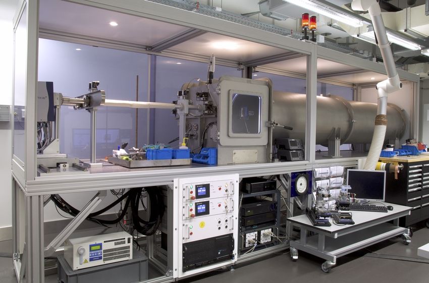
2021 JINST 16 P06034
Figure 1. The MOUSE instrument in its current form, with outer dimensions of 5 × 1.5 × 2 m (Length ×
Width × Height).

comprehensive, universal data correction methodology has been developed that can reliably deliver
“good” data for a wide spectrum of samples (that is to say, data can be obtained in absolute units
with uncertainties, emphasising the true value of the datapoints), and this correction methodology
is now being applied to data from both laboratory- as well as synchrotron-based instruments [3, 5].
 This data correction methodology, however, is useless without the provision of accurate in-
formation (metadata) utilised for the corrections, and needs to be integrated within an overar-
ching measurement methodology, coupled with instrumentation capable of accurately generating
the necessary metadata. This holistic systems architecture approach forms the MOUSE project
(Methodology Optimization for Ultrafine Structure Exploration1), thus consisting of a methodol-
ogy component and an instrumental component. The methodology component of the MOUSE is
composed from a multitude of good operating practices adapted from instruments and research
groups around the world, whereas the instrumental component has been realized as a customized
machine that is continually being modified to improve the measurements.
 To assist in the neverending development of the MOUSE, a high-quality, fully traceable labora-
tory small-/wide-angle X-ray scattering (SAXS/WAXS) instrument forms the crucial instrumental
component (hereafter referred to as the MOUSE instrument). Its experimentally relevant details
are briefly summarized in appendix A, and its comprehensive design considerations are provided
in appendix B. Its specifications exceed the typical requirements for a SAXS/WAXS instrument,
so that various elements of the MOUSE project may be thoroughly proven in practical application.

 1“Ultrafine” here defined following the Oxford dictionary definition: “extremely fine in size, texture, composition, etc.”

 –2–

That is to say, the methodology as well as the instrumentation developed in the MOUSE project is
used for — and tested against — a wide range of samples, to see if limits or exceptions to the as-
sumed universality of the methodology can be explored. To increase chances of finding such limits,
the samples that are measured using the MOUSE originate both from internal institutional sources
as well as from an extensive range of external collaborators. This comprehensive testing could not
have been achieved without the provision of a dedicated (instrument) scientist able to apply the
MOUSE methodology to a wide range of materials science projects, as well as to recognize and
understand failings of the methodology, should they occur. The success of such a holistic approach,
as well as the spectrum of its application, can be evaluated from the rich variety of an increasing
number of papers to which the MOUSE has already contributed to. [6–20]

 2021 JINST 16 P06034
 qmin, Cu
 108
 qmin, Mo
 106
 I ((m·sr)−1 )

 104 qmax, Mo
 qmax, Cu
 102

 1010
 0
 -2 10-1 100 101 102
 q (nm−1 )

Figure 2. A MOUSE project dataset from a ZIF-8 powder sample consisting of ≈ 35 nm particles, measured
using two different X-ray sources (yellow: copper, blue: molybdenum). This dataset combines data from
twelve different instrument configurations (six using copper, six using molybdenum). When using the
molybdenum source, fluorescence from zinc is visible. The instrumental smearing is different for the
different configurations, which will need to be accounted for in any analysis model (rather than attempting
to mathematically de-smear the data, as discussed in our previous work [5].

 In this paper, we will first elaborate on the characteristics of what, we believe, constitutes
“high-quality” X-ray scattering information (this being the ultimate goal of the MOUSE project).
This is followed by a brief exposé on how these characteristics have been addressed in relation to
the MOUSE project, accompanied by example datasets collected using the MOUSE (experimental
details for these examples can be found in appendix A, datasets themselves are available on Zenodo
at [21]). A description of the measurement workflow that has been established around the instrument

 –3–

is also included, as it demonstrates what steps are required to put the underlying MOUSE principles
into practice. Lastly, the many appendices contain detailed information on several aspects of the
instrumentation and the methodology that likely extend beyond the interest of the majority of the
intended readership. However, the interested reader is encouraged to delve into particular aspects
that are described in (extensive) detail there, perhaps somewhat reminiscent of the “choose-your-
own-adventure” class of literature.

2 The essence of quality

The MOUSE project goal is to generate scattering information that could be considered to be of

 2021 JINST 16 P06034
high quality (cf. section B). This requires, however, a brief consideration on what might constitute
high-quality information or a high-quality dataset.
 High quality information may include the following:
 A. Methodology: data collected using a comprehensive and well-documented measurement
 methodology;

 B. Flexibility and Wide -range: the instrument should be able to handle as broad a range
 of samples as possible, but any modification to the benefit of flexibility that may negatively
 impact the data quality should be considered very carefully (e.g. air gaps or the introduction
 of windows in the beam). The data should also be measured over as wide a range as possible
 to ensure overlap with other instruments, and allowing for a comprehensive look at the sample
 in question;

 C. Statistics: determination and minimization of datapoint uncertainty, i.e. where the signal-to-
 background ratio has been maximized, and a sufficient number of sample-scattered photons
 have been counted;

 D. Traceability and Uncertainties: the data is accompanied with reasonable data uncertainty
 estimates, with a documented reasoning behind their derivation, whilst the traceability has
 been considered for its measurands, and can be traced back to primary physical standards;

 E. Corrections: a comprehensive data correction chain with all the relevant parameters and
 values for the corrections are considered, and accessible alongside the data;

 F. Data requirements: open, FAIR and accreditation: data is stored in an open data con-
 tainer, accompanied by all relevant metadata necessary to understand the measurement, and
 troubleshoot potential causes of error; thus, the data adheres to the FAIR principles (Findable,
 Accessible, Interoperable and Reusable), and is catalogued in a comprehensive library; the
 data can (eventually) be supplied with certificates, with the laboratories and instruments ac-
 credited by internal and external quality assurances, as proxies to enable laypersons to apply
 a degree of trust to the data.
 The end result is a dataset that holds sufficient information for experts to assess and determine
what level of trust they would assign to each dataset, and optimally contains additional certificates
to allow laypersons to assign trust. Each of these aforementioned requirements will be discussed
individually, explaining how they have been addressed in the MOUSE project.

 –4–

2.1 Methodology
An under-highlighted but critical aspect of a well-run instrument is the organization surrounding
the measurements. This defines whether past measurements can be found based on e.g. sample-,
user-, or time-information, if all important parameters of that measurement can be read, whether
the applied data correction procedures can be retraced, and if the data analysis methods that were
used to evaluate the data can be reinterpreted.

 Start

 2021 JINST 16 P06034
 Proposal /
 User discussions
 sample form

 Electronic Experiment
 logbook design

 Measurement Datafiles

 SciCat data
 catalog
 Datafile
 conversion, HDF5: NeXus /
 aggregation & NXSAS
 annotation

 HDF5:
 Data correction
 NXcanSAS

 Jupyter (Python)
 Data analysis Analysis output
 notebook

 Finish

Figure 3. General measurement workflow for experiments on the MOUSE. The SciCat data catalog is in
advance stages of development, but not fully integrated as of yet.

 The manufacturer-supplied software that accompanied the MOUSE has been largely replaced,
apart from the SPEC control system and several custom scripts. The following procedure, graphi-
cally depicted in figure 3, is performed for measuring a given sample.
 Firstly, the experiment is documented in a proposal form (consisting of a machine-readable
excel-sheet). This proposal form contains information on the investigator, their project, and what
the investigator is trying to (dis)prove by means of the SAXS/WAXS measurements. Experienced
users can also supply information on the size range of interest, and on the accuracy with which this
determination is to be done. The proposal form also requires the entry of sample information, in-
cluding estimates of the (atomic) composition and gravimetric density for every sample component.
These are used to automatically calculate the X-ray absorption coefficient, , which in turn can be

 –5–

used to determine the irradiated effective sample thickness by way of the measured sample X-ray
transmission. This has proven useful for powders and foil-shaped samples, but also for determining
the effective sample thickness in capillaries.
 Secondly, the most optimal sample measurement geometry is defined in discussion with the
investigator. This sample geometry is largely defined by the restrictions of the X-ray scattering
experiment, but can be adapted to more closely match the normal experimental conditions of
the researcher.
 The measurement parameters and configurations required to fully characterize the sample(s)
in question are entered in a digital logbook (a second, machine-readable excel sheet), with one

 2021 JINST 16 P06034
measurement series in a given configuration per row. When ready, the new rows are automatically
converted to a SPEC measurement script, which ensures that the correct instrument configuration
is set, that all the required steps for a correct measurement are performed, and that all required
metadata will be present in the resulting file. A measurement row defines a series of measurements
in one instrument configuration, i.e. the resulting data contains a number of repetitions of the
measurement, each containing a separate flux, transmission factor, etc.
 The metadata that is measured by the SPEC script alongside every repetition of a measurement
includes:

 • The direct beam profile on the detector (this, by exception, is currently measured only once
 per instrument configuration)

 • The primary beam flux 0

 • The primary beam center

 • The transmission factor of the sample

 • The source parameters (energy, voltage, current)

 • The actual slit parameters

 • All motor readouts, e.g. slit, beamstop, and sample positions, etc.

 • All detector metadata provided by Dectris in their NeXus format, such as energy threshold
 settings, flatfields and countrate correction information

 • The vacuum chamber pressure

 • The interferometer strip readout

 Additional metadata is also collected and stored alongside the data. This includes metadata
inserted (after data collection) from the logbook, such as:

 • The sample name

 • The sample ID (links back to the proposal, also in the catalog)

 • The proposal ID

 –6–

• The operator name

 • The associated background measurement file

 • The associated mask file

 • The overall sample X-ray absorption coefficient

 By following this procedure, logbook-keeping forms an integral part of the instrument opera-
tion. This ensures that all the measurements are automatically performed with the utmost care, and

 2021 JINST 16 P06034
that the logbook is always correct; no logbook entry, no measurement. This makes the logbook
an accurate reflection of the configuration of the measurements. The SPEC measurement scripts
generated by this logbook information were not stored until recently. The thinking here was that,
if the measurement script turns out to be inadequate, this is clear from the lacking metadata in the
final NeXus measurement data. Additionally, all Python code, including the one used to generate
these measurement scripts is mirrored on an institutional versioning repository (Git), and so the
SPEC measurement scripts of a particular date could be regenerated as needed. In the interest of
simplifying this process, however, we are now also storing the SPEC scripts.
 At the end of the measurement series, the data is transferred to the host institute’s network-
attached storage (also for back-up purposes). Subsequently, the data from the instrument is
combined and reformatted into properly annotated raw NeXus files and catalogued in our pro-
totype SciCat database (a copy of the SciCat database system under development at the ESS
(https://scicatproject.github.io/). The measurements are then processed in parallel using DAWN,
and the resulting “derived” datafiles are catalogued in the database, linking back to the original raw
files, alongside some relevant scientific metadata extracted from the files (see figure 3). Once these
processed files are available, the bespoke (and often most laborious) analysis and interpretation
process can begin. . .

2.2 Flexibility and wide q-range

2.2.1 Flexibility
While some instruments (and in particular those in the protein scattering community) have been
meticulously tuned for measuring one class of samples very well, samples in materials science tend
to come in a variety of unique shapes, sizes, states and conditions. Designing an instrument for
increased flexibility from the onset means that fewer concessions need to be made when measuring
such a range of non-standard samples. Fewer concessions lead to fewer sources of error, and this, in
turn, leads to better data. This justification does come at the condition, however, that the increased
flexibility cannot come at the cost of data quality. The flexibility of the MOUSE instrument,
therefore, is a limited flexibility compared to, say, the I22 beamline at the Diamond Light Source.
Many sample geometries, conditions and states can be accommodated in the oversized sample
chamber of the MOUSE, but the chamber must be evacuated before measurement.2

 2That means that for the (so far, small) subset of samples that absolutely require an atmosphere, a custom-built
compact environmental chamber must be developed. Such a cell is currently being designed.

 –7–

2.2.2 Wide q-range

Measuring over a wide-range is essential for both flexibility as well as high-quality data: to get
a comprehensive understanding of a material’s structure, multiple levels must be simultaneously
assessed (one example of such a multi-level analysis is given in [22], albeit with this instrument’s
predecessor). These also serve as a double-check for the validity of the data, e.g. when measuring a
composite containing metal oxide nanoparticles, the corresponding diffraction peaks must also be
present. The wide range is achieved in the MOUSE mainly by virtue of its movable detector, i.e.
by moving the detector closer to or further away from the sample, different ranges of the scattering
vector can be obtained. Additionally, by switching between the copper and the molybdenum

 2021 JINST 16 P06034
X-ray sources, different scattering vector ranges become accessible. For obtaining greater wide-
angle ranges, the detector can also be moved laterally, making high scattering vectors up to almost
100 nm−1 accessible. The resolution at these larger vectors is not great, however, and its performance
as an XRD instrument is not as good as what can be obtained from dedicated diffractometers. This
is due to, amongst others, the high angle of incidence of the scattered radiation and its detection
at the detector plane, the parallel beam dimensions at the sample position in combination with the
typical sample thickness, and the lack of a sample “spinner” for improved bulk averaging.
 To combine the data from multiple scattering vector ranges, a method has been developed that
merges datasets weighted by the uncertainty of their datapoints (described in detail in appendix D).
As the data is already in absolute units after correction, this merging can be done without the
addition of dataset scaling factors. Care must be taken to check for the prominence of effects of
beam smearing before merging, and when these effects are significant, data must be collected using
the same collimation settings, optimized for the longest sample-to-detector distance, before data
merging can take place.

2.3 Statistics

It is critical that a measured signal is as noise-free as possible (maximizing the signal-to-background
ratio), to minimize the signal degradation that occurs during the background correction. Performing
the background subtraction becomes exponentially more challenging with high background levels,
strongly amplifying the resultant data uncertainties. Hence, even if an ostensibly useful signal is
extracted, the propagated uncertainty estimates may have reduced its usability to zero.
 A deliberate choice was made to forego provisions for in-air sample environments, as this
would require the installation of two additional windows and an air path, all of which would add to
the instrumental background signal. For the few samples that do require an atmosphere, a compact
flow-through environmental cell is currently under development. The current configuration consists
of a continuous, windowless vacuum from before the first set of slits to the detector. With the first
series of Dectris Eiger detector, which only has a single low-energy threshold filter, the main
background contribution is that of the cosmic radiation at a rate of 1.43 × 10−5 counts per pixel
per second, which strongly determines the minimum scattering level that can be observed. Whilst
an algorithm was provided by the instrument manufacturer to remove cosmic radiation from our
detected images, the mathematical underpinnings of this procedure remain undocumented, and can
therefore not be included in a traceable, fully open source data correction methodology.

 –8–

Typically, solid (slab-geometry) samples are mounted over holes in a laser-cut template, taking
care that the measured area is tape-free. Powders are sandwiched in the holes of the template
between two sheets of Scotch Magic Tape™, which was found to give a low scattering signal.
Liquids are measured in flow-through cells that either uses two thin, low-scattering silicon nitride
(SiN) windows, which are virtually noise-free and have a transmission factor close to 99%, or
extruded borosilicate capillaries, which have a transmission factor of around 70% for Cu radiation.3
The apparent thickness of these cells is determined using a known absorber (typically water) for
each set of windows and each capillary.

 2021 JINST 16 P06034
2.3.1 Low-noise/detection limits

Defining limits of detectability for the MOUSE instrument, i.e. determining its ability to detect the
signal from a given analyte before an experiment is attempted, requires consideration of multiple
intertwined features. These features can be grouped into three classes: those pertaining to the sample
properties, those arising from various background contributions (normalized by the primary beam
flux), and aspects relating to the quality of the collected data and metadata. Only a short summary
of these contributions is provided bellow, however a more thorough discussion can be found in
appendix F.
 In brief, the first class includes the sample properties of scattering contrast, the analyte concen-
tration and geometry. The second class contains various backgrounds that have to be considered,
in particular backgrounds arising from beam spill, parasitic scattering, cosmic radiation, and the
scattering of the sample container. Added to this are sample-related backgrounds, such as the
scattering signal from the dispersant itself, and backgrounds from potentially fluorescing elements
in the analyte or dispersant. The third class of features, defining the detectability, involves the
accuracy with which the data (including its associated metadata such as flux, time, and transmission
factors) can be determined.
 Practically, the overall background levels have been quantified for various sample environments
in the MOUSE instrument, and are shown in figure 4. Using the current data correction procedures,
and given the current quality of associated metadata, we consider that it is possible to detect an
analyte signal with a magnitude no less than ca. 10% of the background signal. At low , the
instrument background is dominated by the instrumental beam spill and/or tape signals. At higher
 , the cosmic radiation background defines the absolute lower limit for freestanding samples, but
is dwarfed by the signals for tape (used for powder samples) or the water dispersant in the SiN
low-noise flow-through cell. Successful subtraction of the dispersant signal with low-scattering
analytes, puts exponentially higher demands on the accuracy of the coincidental measurands (e.g.
incident flux and transmission factors), and demands the propagation of uncertainty for a confident
analysis later on. Possible strategies for low-scattering analytes in such samples are discussed in
appendix F.

 3Flow-through capillaries are used so that an empty capillary and the dispersant background can be measured in the
exact same capillary before the sample measurement is recorded. This is the only way to ensure correct, problem-free
background subtraction for samples in capillaries.

 –9–

Merged background signals Approximate model background signals
 (for a nom. 1 mm sample thickness) (for a nom. 1 mm sample thickness)
 106 Instrument backgroud + Darkcurrent Instrument background + Darkcurrent
 Tape backgroud Tape background
 105 Water background + SiN cell H2 O at 293K, 105 Pa
 104
 103
I ((m·sr)−1 )

 102
 101
 100
 10-1

 2021 JINST 16 P06034
 10-210-2 10-1 100 101 10-2 10-1 100 101
 q (nm−1 ) q (nm−1 )

Figure 4. Left figure: total background signal levels for the MOUSE instrument, combined from mea-
surements using different instrument configurations shown in figure 21, which an analyte scattering must
contribute significantly to. To use these figures, simulate the analyte scattering in absolute units, multiply
with the sample thickness in mm, and then compare the resulting simulated curve with the above. The analyte
signal should add at least 10% to the background signal.

2.4 Traceability and uncertainties
Traceability refers to whether the measurands of the instrument can be traced back, in an unbroken
chain, to a standard. This is inherently coupled with an estimation of the uncertainty throughout the
chain for this measurand. When an X-ray scattering instrument is demonstrably traceable, in both 
and , it adds reliability to the values obtained, and an accuracy that those values can be determined
within. This enables such an instrument to be used to calibrate and certify samples, which, in turn,
can then be used to calibrate other instruments.
 This effort has been undertaken for the MOUSE instrument, which is expanded upon in detail
in appendix C. There, it is shown that both the scattering cross-section, , as well as the scattering
vector, , can be traceably defined, within reasonable levels of uncertainty (5% for the scattering
cross-section, and a configuration-dependent uncertainty at best below 1%) for the MOUSE
instrument. The traceability of the scattering cross-section is shown to be determinable using the
detailed data correction methodology, without referring back to calibrants. The traceability of the
scattering vector is determined using a triangulation method coupled with a traceably calibrated
laser distance measure and an interferometer strip alongside the motorized detector carriage.

2.5 Corrections
As many corrections as possible are applied to the collected data. These have been comprehensively
described in our previous work [5, 23], and are implemented in the DAWN software package [24].
As discussed in [5], other tools are also available for data correction (e.g. ATSAS [25], DPDAK [26],
PyFAI [27], pySAXS [28], Xi-CAM [29], FOXTROT [30]). However, we found these to be limited in
the number and extent of implemented corrections and/or in their uncertainty propagation. Most also
lacked the ability to adjust and re-order the individual correction steps. PyFAI, however, will likely
be integrated as a part of our modular corrections as a faster implementation of the averaging steps.

 – 10 –

We now also include an automated calculation of the X-ray absorption coefficient based
on the atomic composition and density of the sample components, which allows for an automatic
calculation of a sample’s apparent thickness based on the measured X-ray absorption. Currently, only
one correction has not yet been implemented: the deadtime correction. At the time of this writing,
this correction is performed on the data by the detector software itself, which negatively impacts the
accuracy of the uncertainty estimation. At issue here is the uncertainty estimates that derive from
the counting statistics. These need to be estimated based on the actual number of detected counts,
and not on the hypothetical number of incident counts obtained after the deadtime correction. For
this reason, efforts are underway to disable this correction in the detector software, allowing us to
determine a better estimate for the counting uncertainties. After this estimation has been performed,

 2021 JINST 16 P06034
the deadtime correction can be applied and the uncertainties propagated through the corrections.
 Besides this, however, the correction sequence described in our previous work has consistently
delivered data without obvious data correction flaws (such as over- or under-subtracted backgrounds)
irrespective of the type of samples. This universality has been demonstrated for measurements both
on our instrument as well as at the I22 beamline at the Diamond Light Source, where the same
correction sequence is used to treat their data [3]. It functions well for both strongly- and weakly
scattering samples, solids, composites, liquids, as well as powders, the latter of which form a
surprisingly large fraction of the samples we have measured.
 Upgrades currently underway concerning the MOUSE correction sequence include an auto-
mated calculation of the scattering cross-section based on the density and atomic composition of
the components within each sample to aid in automation of the analysis. Future upgrades will
include automatic flags to highlight potential issues at an early stage. These flags could indicate
common issues such as a strong probability for multiple scattering, transmission factors that are too
low or too high (too much or too little sample in the beam, respectively), large uncertainties after
correction, and incident beam instabilities.

2.6 Data requirements: open, FAIR and accreditation
2.6.1 Open data format
Any dataset loses value when it cannot be read by everyone, or when it can no longer be read at all.
Such data loss becomes particularly painful when the data is required for checks or reinterpretation
after publication. All recorded data should, therefore, be stored in a suitable, stable open-source
archival dataformat. One such format, is the HDF5-based NeXus container, which is flexible,
reasonably fast, and can comprehensively store all imaginable formats and shapes of data, alongside
its associated metadata, in a clear, self-describing, hierarchical structure [31, 32].
 In the case of the MOUSE, all data collected from a series of measurements collected in a
single instrument configuration for a given sample, is combined into a single “raw” HDF5/NeXus
file. The information in this file is decorated with metadata from the instrument as well as
measurement information extracted from the electronic logbook,4 and recently also includes sample
information extracted from the SciCat database. The aforementioned data processing, which the
“raw” files undergo, utilises this HDF5/NeXus file structure. This structure allows for input data and
 4As the same logbook is used to automatically generate the measurement script, the information in the logbook has a
high degree of reliability.

 – 11 –

metadata to be read, but also means that the processing tree can be stored alongside the original and
processed data, in a new “derived” datafile. Subsequently, analyses could also be stored within the
HDF5/NeXus file structure, generating a comprehensive, traceable overview on how conclusions
were derived from the measurement data.

2.6.2 FAIR
Having your data stored in a way that can be read is one thing, but the story doesn’t quite end there.
Good data stewardship — yet another task befalling upon good researchers — also requires that 1)
you can find the data again at an unknown time in the future, that 2) it is made accessible to others,

 2021 JINST 16 P06034
and 3) that they can reuse it for their own research. In full, the principles of data stewardship can
be summarized using the four FAIR guiding principles [33, 34]:

 • Findable: metadata and unique identifiers should be added to the data, which should be
 uploaded in a searchable database. We currently do this by uploading to our internal SciCat
 database.

 • Accessible: the database should be made accessible to others using common protocol(s),
 with at a least searchable metadata, even if the data itself is not searchable. Currently our
 development database is accessible from within the organization, but not from outside (yet).

 • Interoperable: data and metadata should be described using clear and consistent vocabulary,
 with appropriate references provided where possible. We are following the nomenclature as
 defined by the canSAS data format working group, codified in the NXcanSAS application
 definition (https://manual.nexusformat.org/classes/applications/NXcanSAS.html).

 • Reusable: the data should be accompanied with metadata and appropriate information to give
 it provenance. The format of that this information is presented should adhere to community
 standards. We achieve this through utilisation of the NeXus data format and our detailed and
 documentation-enforcing workflow.

 In summary, we are on our way to improve our data stewardship, but developments are still
ongoing.

2.6.3 Accreditation
There are two ways of finding out if the data from an instrument can be trusted. The first and
best way is for experts to check the metadata of the measurement and the instrument, to make an
educated assessment on the data quality and reliability. This, however, requires the availability
of a trustworthy expert with the time to thoroughly examine datasets and investigate instruments
(insofar as possible). The job of the expert can be made much lighter by ensuring this information
is present, either as metadata in the datafiles themselves, or in written (long)form accompanying
the measurements.
 A second method for trust is trust by proxy, and works better for well-established, widespread
techniques such as electron microscopy or UV spectroscopy. In these cases, an independent
adjudicator is hired to verify that the appropriate standards for measurement and documentation are

 – 12 –

adhered to. If so, a certificate can be bestowed upon the technique and laboratory, which is usually
considered a trustworthy proxy for quality that can be assessed by anyone.
 In case of the MOUSE, there are only a limited number of standards it can adhere to. There is
a ISO standard for the analysis of particle size by small-angle X-ray scattering (ISO 17867), which
describes the technique and highlights some analysis methods. Besides this, there are ISO 17034
(General requirements for the competence of reference material producers) and ISO 17025 (Gen-
eral requirements for the competence of testing and calibration laboratories), which together with
GxP (“good practice”) and CMC (Chemistry, Manufacturing and Control) analytical procedures
and method validations, provides a framework for managing measurements on instrumentation in
general. This available set of standards and guides has been used in the development of a compre-

 2021 JINST 16 P06034
hensive measurement methodology for the MOUSE. However, since the focus of the instrument lies
in research rather than testing at the moment, certificates of conformity by independent adjudicators
have not (yet) been pursued.

3 Experimental Examples

As mentioned in the introduction, the MOUSE has successfully been applied to a very wide range
of materials science-relevant samples. This can be demonstrated by means of a few examples. The
general experimental details used for these measurements can be found in appendix A.

3.1 Alumina membranes
The first example shows the applicability of the MOUSE to aid in materials science investigations.
Here, the scattering from a porous alumina membrane is shown, these membranes are similar
to those described in detail in Yildirim et al. [6]. These contain a hexagonal array of pores
perpendicular to the surface plane (conforming to a P6mm spacegroup). In these membranes, the
pore spacing is nominally 65, 125 and 480 nm (with a manufacturer-specified standard deviation
of less than 10%), and the pore diameter 40, 50, and 180 nm, respectively. These membranes have
an approximate thickness of 100 μm. The peak positions in the scattering patterns (figure 5) can
be identified using peak finding methods, with their position optimized for a hexagonal lattice of
the P6mm spacegroup, indicating lattice spacings of 64 and 119 nm for the smaller pitches (the
largest, with a nominally 480 nm pitch, cannot be accurately determined at this stage). Given their
high reproducibility, they may lend themselves well as q-calibration materials for low-q vectors in
non-traceable instrumentation.

3.2 ZIF-8 and porous carbon catalysts
The second example demonstrates the wide-range, dual-source capabilities of the MOUSE, and
consists of two samples. The first of the two are ZIF-8 nanoparticles, synthesised in-house using
procedures detailed in [35]. Through accurate control of the synthesis conditions, the final particle
size has be kept small, and the size distribution narrow. The sample was measured as a dried powder
(figure 6), and shows the expected increase in fluorescence from zinc when using the molybdenum
source at wide angles. The small-angle region can be fitted to obtain a size distribution, whereas
the wide-angle region can be indexed to verify the structure and phase purity of the ZIF-8 powder.
The background subtraction procedure improves the wide-angle signal, which, in turn, is beneficial

 – 13 –

1011

 109

 107
 I ((m·sr)−1 )

 105

 2021 JINST 16 P06034
 103 x 50
 CWT-detected peak positions x1
 101 P6mm model peak positions
 Alumina membrane P65 D40
 Alumina membrane P125 D50 x 0.02
 10-1 Alumina membrane P480 D180
 10-2 10-1 100 101
 q (nm−1 )

Figure 5. Scattering from hexagonal arrays of pores in 125 and 65 nm pitch alumina membranes, and a
trigonal array of pores with a 480 nm pitch, similar to those previously discussed in Yildirim et al. [6].
Vertical lines indicate the uncertainty (±1 SD) on the datapoints. Red downward triangles indicate detected
peak positions, black downward triangles indicate fitted peak positions for P6mm arrays with 119 nm pitch
and 64 nm pitch for the indicated 125 and 65 nm pitch membranes, P125 and P65, respectively. The scattering
signals of the 65 nm and 480 nm pitch membranes have been shifted for clarity by a factor of 50 and 0.02. For
the 480 nm pitch membrane, information on the hexagonal array is only barely visible at low-q. (Alumina
membrane samples courtesy of Dr. Arda Yildirim, BAM, DE)

for the analysis. The second sample to demonstrate the wide-range, dual-source capabilities of the
MOUSE is a porous carbon matrix with embedded iron carbide nanoparticles. This type of sample
is described in detail in [9]. In contrast to the previous samples, these contain a high fraction of
metal carbide additives. Of interest is not just the extension of the small-angle region into the
XRD region, thereby serendipitously providing X-ray diffraction (XRD) data in absolute units with
uncertainty estimates, but also the drastic differences in signal that a multi-source set-up can bring
for fluorescing samples.

3.3 Tobacco Mosaic Virus
To demonstrate the flexibility of the instrument, as well as the limits imposed by the background,
a biological sample was measured in dispersion. The liquid dispersion contains an amount of the
tobacco mosaic virus (TMV), which is a helicoidal, elongated structure, whose envelope resembles
a cylinder with a diameter of ca. 18 nm, and a length of ca. 300 nm [36]. The resulting curve, shown
in figure 7, is compared to a curve simulated using the SPONGE. This is an in-house developed
Python software package, that loads a 3D closed surface in the STereo Lithography (STL) format,

 – 14 –

1010
 ZIF-8 measured with copper radiation Fe3C-containing catalyst Cu-source data
 ZIF-8 measured with molybdenum radiation Fe3C-containing catalyst, Mo-source data
 108

 106
I ((m·sr)−1 )

 104

 102

 1010
 0
 -2 10-1 100 101 102 10-2 10-1 100 101 102
 q (nm−1 ) q (nm−1 )

 2021 JINST 16 P06034
Figure 6. Left: scattering from a ZIF-8 powder sample consisting of ≈ 35 nm particles, measured using
two different X-ray sources. With use of the molybdenum source, fluorescence from zinc is observed.
Right: a highly porous carbon sample containing small amounts of iron carbide nanoparticles. The iron
carbide shows fluorescence when using the copper source (sample courtesy of Dr Zoe Schnepp, University
of Birmingham, GB).

 106 Tobacco mosaic virus
 Total background (instrument + cell + water)
 105 sasModel cylinder, 16 nm dia., 300 nm length.
 Simulated scattering of two 17.6 nm diameter TMV segments
 104
 I ((m·sr)−1 )

 103
 102
 101
 100
 10-1
 10-2 10-1 100 101
 q (nm−1 )

Figure 7. Tobacco mosaic virus scattering pattern, and the corresponding model pattern from simulated data
using the SPONGE as well as from a cylinder of length 300 and diameter 16 nm calculated using sasmodels.
A 16 nm diameter cylinder was selected as a simplified approximation of TMV to remove the capsomer
protrusions (TMV sample courtesy of Prof. Ulrich Commandeur, RWTH Aachen University, DE).

 – 15 –

and computes the scattering pattern using the Debye equation on randomly distributed points
within the surface. The SPONGE estimates data uncertainties and allows for size distributions and
dynamics to be considered, as shown in our recent work on other helical structures [37].
 Here, due to the large dimensions and the fine detail, only a 180-nm-long subunit of TMV was
simulated, leading to deviations at low- -values (< 0.07 nm−1 ). The remainder of the scattering
curve is described well by the simulation. The TMV subunit STL model was created by Nuansing,
provided under a CC-BY 3.0 license [38]. To describe the overall, large-scale structure of the TMV,
the scattering of a cylinder of the correct dimensions has been shown alongside, better describing
the low- behaviour. This cylinder scattering shows that very little information on the length of the

 2021 JINST 16 P06034
cylindrical structure may be available in the measured range. Furthermore, it bears repeating that the
uncertain scattering observed at low is due to the relatively high instrumental background (beam
spill) signal compared to the low TMV signal at those angles. At high , the intensity decrease is
uncertain due to the low analyte signal level compared to the (5-10 times higher) scattering of the
water dispersant, making it exponentially more unlikely to successfully extract the correct signal
even with the methods presented herein (cf. appendix F).

3.4 NIST gold nanoparticles RM8011

The correctness of the MOUSE traceability was re-verified using nominally 10 nm gold nanopar-
ticles from NIST under catalog number RM 8011 (figure 8). A previously used sample of this
material was available in the laboratory, and was measured in a low-noise flow-cell under contin-
uous recirculation. For the background measurement, water was measured in the same low-noise
flow cell prior to the sample measurement. Measurements were performed in several instrument
configurations to obtain a wide range scattering pattern, with a total scattering pattern recorded over
a timespan of 6 h for the background and 12 h for the gold sample. The noise levels at low are
large due to the magnitude of the beam spill versus the minimal sample signal at those scattering
vectors. At high , the noise is due to the low analyte signal level compared to the scattering of the
water dispersant.

 106 7000
 Corrected Gold NP data McSas number distribution, 2 R 7
 Total background (instrument + cell + water) SasView distribution
 McSAS fit 6000
 SasView fit
 104
 number fraction (A.U.)

 5000
 4000
I ((m·sr)−1 )

 102
 3000
 100 2000
 1000
 10-2
 0
 10-2 10-1 100 101 1 2 3 4 5 6 7 8
 q (nm−1 ) nanoparticle radius (nm)

Figure 8. Left side, data, background level, McSAS and SasView fits of the NIST RM 8011 gold nanoparticle
dispersion. Right-hand side, comparison between the number-weighted distributions obtained through
SasView and McSAS over the radius range of 2–7 nm (sample courtesy of Dr. Andreas Thünemann, BAM,
DE). Vertical black lines indicate the uncertainty (±1 SD) on the datapoints. (The background shown is
identical to that from figure 7 as the same cell, background material and configurations were used.)

 – 16 –

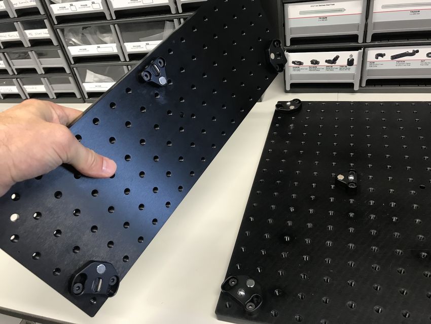
The gold measurement was analyzed using the software packages McSAS and SasView. Mc-
SAS was applied assuming spherical scatterer geometry between 0.1 ≤ (1/ ) ≤ 7, and the
resulting size distribution quantified between 2 ≤ ( ) ≤ 7, to avoid contributions from ag-
glomerates and flat background. SasView was applied assuming spherical scatterer geometry and
a normal size distribution, between 0.01 ≤ (1/ ) ≤ 0.7, with a dataset scaled to the appropriate
SasView units of (cm · sr) −1 (as opposed to the standard (McSAS) units of (m · sr) −1 . The results
from the fits (available in the SI), show narrow dispersities with mean radii agreeing well with the
NIST-specified values as obtained using AFM: 8.5 ± 0.3, and TEM: 8.9 ± 0.1. McSAS shows a
mean (number-weighted) diameter of 8.55(2), SasView shows 8.60 nm. The concentrations are
about 7% higher as found both with SasView and McSAS as the specified (non-reference) value of

 2021 JINST 16 P06034
the documentation of 51.6 μg/ml, with McSAS giving 55.3 μg/ml and Sasview 54.8 μg/ml.
 The volume fraction deviates a little more than expected from the reference values. Fortunately,
the sample was measured over multiple repetitions, and later repetitions revealed steadily increasing
volume fractions, with the third repetition giving concentrations of 63.2 μg/ml and 63.3 μg/ml for
McSAS and SasView, respectively, a 20% increase over the target value. It was found after the
experiments that there was a significant coating of gold on the SiN windows of the flow-through
cell, so we here find that the increase in observed concentration can likely be ascribed to the
long measurement times (12 h per measurement) and the sticking of gold nanoparticles to the cell
windows. Additionally, as the sample had been opened before, the initial concentration can also
have increased due to some evaporation of the solvent over time. In addition to these effects, the
presence of a small fraction of agglomerates is detected, in particular when comparing the intensity
at low angle of these measurements compared to those of [39]. While these agglomerates are not
expected to increase the observed concentration, they do hint towards changes of the sample over
time. A more accurately determined volume fraction standard could be developed for improved
calibration and verification of scattering instruments. Overall, however, the sample underscored the
accuracy of the MOUSE methodology.

4 Outlook and conclusions

With the MOUSE project now suitably well developed, high-quality X-ray scattering measurements
are being obtained for a steady stream of samples. Already several thousands of datasets (each
consisting of many repetitions) have been collected in its first two and a half years of development.
Like at synchrotron beamlines, the development of this project is reliant on the right people,
appropriate equipment, as well as a well-structured methodology including proposal forms and data
catalogs. Unlike synchrotrons, however, experiments in a laboratory setting are free to last as long
as necessary (time-wise), and can be repeated easily when they do not work the first time around.
The availability of the MOUSE instrument lowers the threshold for more daring proof-of-concept
measurement strategies or materials investigations without too much pressure, and enables the
development of extensions to both the instrumentation as well as the methodology.
 The MOUSE instrument remains in a constant state of flux, with current efforts focusing on
integrating GISAXS, upgraded sample stages, various heating- and cooling stages, tensile stages and
magnetic- and electric field stages. The future will also see the integration of additional equipment,
including spectrometers and an Ultra-SAXS plug-in module [52]. The MOUSE is also occasionally

 – 17 –

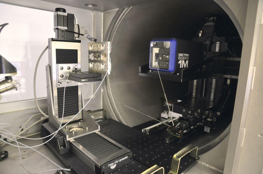
used as an in-line analytical instrument to follow lab-scale syntheses, an application which will be
exploited more frequently in the future. With our efforts on modular improvements to the MOUSE
instrument (e.g. its “M”- and “S”-sized mounts, standardized sample holders, etc.), but also of
the surrounding MOUSE methodologies, we hope to encourage transfer of the knowledge and
experience gained in the MOUSE project to any compatible instrument worldwide, and hopefully
soon too, to a laboratory or synchrotron near you.

Acknowledgments

The authors thank Dr. Ingo Bressler for their work on implementing the fledgling SciCat database,

 2021 JINST 16 P06034
and the team behind SciCat at the European Spallation Source for its development. Furthermore,
we thank Dr. Andreas Thünemann for his input on the manuscript. Dr. Tim Snow and Dr. Jacob
Filik from the Diamond Light Source are thanked for their continued integration and improvements
of the SAXS data corrections in DAWN. Dr. Tim Snow is also thanked for his input on many aspects
of the paper. This work was partially funded through the European Metrology Programme for
Innovation and Research (EMPIR) project No. 17NRM04. Lastly, we thank all the scientists and
collaborators who are the driving force for the continued development of the MOUSE.

A Experimental: a brief introduction to the MOUSE instrument

The upcoming sections will contain practical examples for illustration, this section briefly sum-
marizes the experimental set-up and measurement aspects which will be elaborated on later. The
SAXS/WAXS measurements shown in the examples were performed using the MOUSE: a heavily
customized Xeuss 2.0 (Xenocs, France), installed at the Bundesanstalt für Materialforschung und
–prüfung (BAM), Berlin. The MOUSE uses X-rays from microfocus X-ray tubes, followed by mul-
tilayer optics to parallelize and monochromatize the X-ray beams to a wavelength of Cu = 0.154 nm
for the copper source, and Mo = 0.071 nm for the molybdenum source. These are collimated using
three sets of scatterless slits (two germanium and one silicon, with the latter virtually transparent
to molybdenum radiation, but very effective for copper radiation). The detector is an in-vacuum
Dectris Eiger R 1M on a three-axis motorized platform, for these investigations placed at distances
ranging from ca. 50–2500 mm from the sample. After correction, the data from the different
distances and different sources are combined using a procedure that merges the datasets in such a
way as to optimize the uncertainties in the overlapping regions (cf. appendix D), producing a single
continuous curve.
 The sample-to-detector distance is traceably calibrated using a triangulation method, with the
detector position cross-checked with interferometer strip readings and a traceably calibrated Leica
X3 laser distance measurement device (cf. section C). The space between the start of the collimation
up to the detector is a continuous, uninterrupted vacuum to reduce the instrument background. Pow-
ders are mounted in flat, laser-cut sample holders, between two pieces of Scotch Magic Tape™. The
thickness of the sample holder is selected based on the composition of the sample, with the apparent
sample thickness then calculated based on the measured X-ray absorption, atomic composition and
density of the sample. Liquids are measured either in a flow-through borosilicate capillary, or
within a low-noise SiN-windowed flow cell, both with a fixed pathlength of approximately 1 mm.

 – 18 –

The effective thickness of the liquid cells is determined for each cell, based on the measured X-ray
absorption of water. For liquid experiments, care is taken to measure the background in the same
location within the same cell, using the same beam collimation configurations, before the sample is
injected into the cell.
 By using both photon energies over a range of overlapping sample-to-detector distances, a very
wide range in scattering vectors can be covered, and X-ray fluorescence contributions visible for
some samples can be identified. The resulting data is then processed using the DAWN software
package [24, 40]. For the majority of samples, the following processing steps are applied in order:
masking, calculating Poisson errors, correction for counting time, dark-current, transmission, self-

 2021 JINST 16 P06034
absorption, primary beam flux, instrument and container background, flat-field, detector efficiency,
thickness, and solid angle, followed by azimuthal averaging (cf. [5]). By virtue of the completeness
of the corrections, and by measuring the flux using the direct beam on the detector, the processed
data is in absolute units. Scaling of the individual datasets from the various distances and sources
to achieve overlap is, therefore, unnecessary. Photon counting uncertainties are propagated through
the correction steps, and dynamically masked pixels are stored as metadata alongside the processed
data. The data merging procedure and the uncertainty propagation for , as well as details on an
additional uncertainty estimation for originating from the data merging procedure are provided
in appendix D and E, respectively.

B Design and technical details

In the conceptualization stage of the MOUSE, the following design considerations were made:

 • The X-ray sources should be reliable over bright, to ensure the reproducibility and stability
 during the data collection.

 • At least two X-ray sources should be present, so that energy independence and -switching can
 be demonstrated. Energy switching is useful for samples containing fluorescing elements (Fe,
 Co, Ni, Cu, Zn, etc.), for which either the one or the other source will produce lower-noise
 data.

 • The collimation should consist of scatterless slits, three sets at best to ensure collimation
 flexibility

 • the beam path should be a continuous vacuum from the start of the collimation to the detector
 surface, to minimize the background scattering signal

 • The sample chamber must be very large, to house a wide range of sample environments
 without making concessions on the sample environment design in order to minimize their
 footprint, and to be able to house the future Ultra-SAXS plug-in. The sample chamber
 should come with kinematic feet for standard plates (discussed below), and be equipped with
 sufficient flanges for lead-through connectors.

 • The detector should be a low-noise, photon-counting, direct detection system, capable of
 measuring the direct beam (for traceability reasons, see section C).

 – 19 –