Functional convergence of biosphere-atmosphere interactions in response to meteorological conditions - Biogeosciences
←
→
Page content transcription
If your browser does not render page correctly, please read the page content below
Biogeosciences, 18, 2379–2404, 2021
https://doi.org/10.5194/bg-18-2379-2021
© Author(s) 2021. This work is distributed under
the Creative Commons Attribution 4.0 License.

Functional convergence of biosphere–atmosphere interactions
in response to meteorological conditions
Christopher Krich1,2 , Mirco Migliavacca1 , Diego G. Miralles2 , Guido Kraemer1,3 , Tarek S. El-Madany1 ,
Markus Reichstein1 , Jakob Runge4 , and Miguel D. Mahecha3,5
1 Department   Biogeochemical Integration, Max Planck Institute for Biogeochemistry, 07745 Jena, Germany
2 Hydro-Climate    Extremes Lab (H-CEL), Faculty of Bioscience Engineering, Ghent University, Ghent, Belgium
3 Remote Sensing Centre for Earth System Research, Leipzig University, 04103 Leipzig, Germany
4 Institute of Data Science, German Aerospace Center, 07745 Jena, Germany
5 Remote Sensing Centre for Earth System Research, Helmholtz Centre for Environmental Research – UFZ,

04318 Leipzig, Germany

Correspondence: Christopher Krich (ckrich@bgc-jena.mpg.de)

Received: 8 October 2020 – Discussion started: 21 October 2020
Revised: 15 January 2021 – Accepted: 27 February 2021 – Published: 16 April 2021

Abstract. Understanding the dependencies of the terres-           comprehensive understanding of the state of ecosystem func-
trial carbon and water cycle with meteorological conditions       tioning. Long-term or even irreversible changes in network
is a prerequisite to anticipate their behaviour under cli-        structure are rare and thus can be indicators of fundamental
mate change conditions. However, terrestrial ecosystems and       functional ecosystem shifts.
the atmosphere interact via a multitude of variables across
temporal and spatial scales. Additionally these interactions
might differ among vegetation types or climatic regions. To-
day, novel algorithms aim to disentangle the causal structure     1   Introduction
behind such interactions from empirical data. The estimated
causal structures can be interpreted as networks, where nodes     Terrestrial ecosystems and the atmosphere constantly ex-
represent relevant meteorological variables or land-surface       change energy, matter, and momentum (Bonan, 2015). These
fluxes and the links represent the dependencies among them        interactions result in biosphere–atmosphere fluxes (in partic-
(possibly including time lags and link strength). Here we de-     ular carbon, water, and energy fluxes) that are shaped by a
rived causal networks for different seasons at 119 eddy co-       variety of climatic conditions and states of the terrestrial bio-
variance flux tower observations in the FLUXNET network.          sphere (McPherson, 2007). Understanding how biosphere–
We show that the networks of biosphere–atmosphere interac-        atmosphere fluxes interact and how they causally depend on
tions are strongly shaped by meteorological conditions. For       the short-term meteorological and long-term climate condi-
example, we find that temperate and high-latitude ecosys-         tions is crucial for building predictive terrestrial-biosphere
tems during peak productivity exhibit biosphere–atmosphere        models (Detto et al., 2012; Green et al., 2017). However, the
interaction networks very similar to tropical forests. In times   exact causal structure of dependencies between surface and
of anomalous conditions like droughts though, both ecosys-        atmosphere variables is still subject to unknowns (Baldocchi
tems behave more like typical Mediterranean ecosystems            et al., 2016; Miralles et al., 2019). For example, we still do
during their dry season. Our results demonstrate that ecosys-     not understand well under which conditions certain climate
tems from different climate zones or vegetation types have        extremes turn ecosystems into carbon sources or sinks (Sip-
similar biosphere–atmosphere interactions if their meteoro-       pel et al., 2017; Flach et al., 2018; von Buttlar et al., 2018).
logical conditions are similar. We anticipate our analysis to     One reason for our incomplete understanding is that the
foster the use of network approaches, as they allow for a more    causal dependencies underlying biosphere–atmosphere inter-
                                                                  actions might vary among ecosystems depending on vegeta-

Published by Copernicus Publications on behalf of the European Geosciences Union.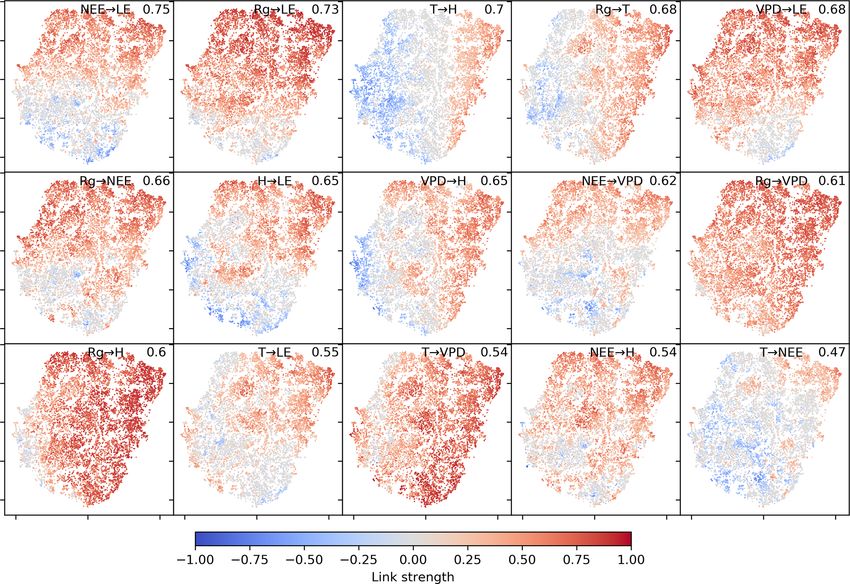
2380                                         C. Krich et al.: Functional convergence of biosphere–atmosphere interactions

tion structure and its long-term adaptation to climatic condi-    first that the accessible states of biosphere–atmosphere inter-
tions.                                                            actions are limited and can be characterised by few functional
   Conducting a comparative study across ecosystems, focus-       states despite the complexity and differences among ecosys-
ing on their interactions with the atmosphere, has two re-        tems. Second, attributing to an ecosystem’s adaptation, we
quirements: firstly, we need standardised data encoding bio-      further hypothesise that a specific ecosystem can only access
sphere fluxes and meteorological conditions. Secondly, an         a limited fraction of the functional states.
analytical tool is needed that extracts an interaction struc-        The study is designed as follows: firstly, we perform causal
ture from these data empirically. The latter requires han-        discovery by PCMCI at each eddy covariance site and sea-
dling of multivariate processes and estimating dependen-          son. Secondly, we solely investigate the resulting interac-
cies beyond correlations. The first requirement is best met       tion networks and visualise them in a low-dimensional space.
by the FLUXNET database (Baldocchi, 2014), a collection           We then interpret the low-dimensional space of biosphere–
of global long-term observations of biosphere–atmosphere          atmosphere interactions and investigate seasonal cycles,
fluxes measured via the eddy covariance method (Aubinet           characteristic states, and the role of vegetation types and fi-
et al., 2012). The spatial distribution of FLUXNET sites is       nally discuss the potential role of adaptation to the underly-
biased to European and North American sites, yet it still cov-    ing climate space.
ers most climate zones and vegetation types ranging from
boreal steppe to tropical rainforests surprisingly well (Reich-
stein et al., 2014). Further, the data are processed homoge-      2     Data and methods
neously across sites. The second requirement is addressed
by causal inference. Various methods exist today (see Runge       2.1    Eddy covariance observations
et al., 2019a, for a recent overview), some of which have
been applied already in the biogeosciences (Ruddell and Ku-       We used eddy covariance data from the FLUXNET database
mar, 2009; Detto et al., 2012; Green et al., 2017; Papa-          (Baldocchi et al., 2001) aggregated to daily time resolu-
giannopoulou et al., 2017; Shadaydeh et al., 2019; Claessen       tion. To maximise the available ecosystems and time series
et al., 2019). One of that group is PCMCI (Runge et al.,          length, we took the union of the LaThuile fair-use (Bal-
2019b), a causal graph discovery algorithm based on a com-        docchi, 2008) and FLUXNET2015 Tier 1 (Pastorello et al.,
bination of the PC algorithm (named after its inventors, Pe-      2020) datasets (Nelson et al., 2020) with at least 5 years of
ter and Clark; Spirtes and Glymour, 1991) and the test of         measurement. If a site year was available in both datasets,
momentary conditional independence (MCI) (Runge et al.,           we selected the one from FLUXNET2015. A detailed list
2019b). By applying such tests, it becomes possible to ac-        of used sites and years is given in Table A1. The final
count for common drivers and mediators which can cause            dataset contains 119 sites from the major plant functional
two variables to correlate even though no direct causal link      types and covers the major Köppen–Geiger climate classes,
exists between them. Then MCI partial correlations esti-          i.e. tropical to polar climate zones. The majority of sites
mated by PCMCI yield a better interpretation of the strength      belong to evergreen needleleaf forests, grasslands, and de-
of a causal mechanism than the common Pearson correla-            ciduous broadleaf forests. The dominant climate classes are
tion. Krich et al. (2020) tested PCMCI regarding its suitabil-    continental, temperate, and dry climates. The dataset’s vari-
ity for interpreting eddy covariance data. The method proved      ables, including meteorological and eddy covariance mea-
to be consistent despite the data’s inherent noisy character      surements, were quality-checked, filtered, gap-filled, and
and was capable of extracting well-interpretable interaction      partitioned with standard tools (Papale et al., 2006; Pas-
structures. A causal interpretation of specific links, though,    torello et al., 2020) and provided with per-variable quality
has to take into account regarding potentially unmet assump-      flags. We extracted the following variables, comparable be-
tions.                                                            tween the two datasets, and their corresponding quality con-
   In this study, we investigate multivariate time series         trols (if available): short-wave downward radiation (or global
from FLUXNET tower data to understand how networks                radiation, Rg ), air temperature (T ), net ecosystem exchange
of biosphere–atmosphere interactions vary across vegeta-          (NEE) (inverted so that positive values signify carbon uptake
tion types and climate zones. The rationale is as follows:        into the biosphere), vapour pressure deficit (VPD), sensible
if biosphere–atmosphere interactions varied significantly         heat (H ), latent heat flux (LE), gross primary productivity
across climate gradients or between vegetation types, this        (GPP), precipitation (P ), and soil water content (SWC, mea-
could indicate, for example, that ecosystem responses to cli-     sured at the shallowest sensor). Within the FLUXNET2015
matic extremes could differ significantly and would require       dataset these variables are named as “SW_IN_F_MDS”,
terrestrial-biosphere models to account for them differently.     “TA_F_MDS”, “NEE_VUT_USTAR50”, “VPD_F_MDS”,
If, however, the opposite applies and ecosystems of the Earth     “H_F_MDS”, “LE_F_MDS”, “GPP_NT_VUT_USTAR50”,
exhibit similar biosphere–atmosphere interaction types, then      “P”, and “SWC_F_MDS_1”, respectively. Correspond-
common principles can be identified that can serve as empir-      ingly for the LaThuile dataset they are “Rg_f”, “Tair_f”,
ical reference for global vegetation models. We hypothesise       “NEE_f”, “VPD_f”, “LE_f”, “H_f”, “GPP_f”, “precip”, and

Biogeosciences, 18, 2379–2404, 2021                                                 https://doi.org/10.5194/bg-18-2379-2021
C. Krich et al.: Functional convergence of biosphere–atmosphere interactions                                                   2381

“SWC1_f”, respectively. GPP is calculated via the com-              defined as unidirectional by the user (PCMCI parameter se-
monly used nighttime flux partitioning (Reichstein et al.,          lected_links; see Table A2). A causal interpretation of links
2005). Here GPP is the difference between ecosystem res-            rests on the standard assumptions of causal discovery. Here
piration and NEE. The latter is estimated via a model which         we assume time order, the causal Markov condition, faith-
is parameterised using nighttime values of NEE.                     fulness, causal sufficiency, causal stationarity, and no con-
                                                                    temporaneous causal effects. The use of ParCorr addition-
2.2   PCMCI                                                         ally requires stationarity in the mean and variance and linear
                                                                    dependencies (Runge et al., 2019b). In particular, a statisti-
To analyse biosphere–atmosphere interactions, we estimated          cal independence (here at a 0.1 two-sided significance level)
network structures using the causal-network discovery algo-         between a pair of variables conditional on the other lagged
rithm PCMCI. PCMCI is tailored to estimate time-lagged de-          variables is interpreted as the absence of a causal link (faith-
pendencies from potentially high-dimensional and autocor-           fulness condition). On the other hand, a causal interpretation
related multivariate time series. Dependencies can be inter-        of the estimated links is here to be understood only with re-
preted causally under certain assumptions. The algorithm is         spect to the variables included in the analysis. The depen-
explained from a biogeoscientific viewpoint in Krich et al.         dence structure among variables can finally be visualised by
(2020). A comprehensive description from theoretical as-            weighted networks with the nodes representing the variables
sumptions to numerical experiments is given in Runge et al.         and the links representing significant dependencies with its
(2019b). As a brief summary, PCMCI efficiently conducts             strengths given by the MCI partial correlation.
conditional independence tests among variables to recon-
struct a dependency network. While PCMCI can also be                2.3   Network estimation
combined with non-linear tests, here we estimate conditional
independence using partial correlation (ParCorr), implying          Dependencies are estimated using PCMCI among the vari-
that we only consider linear dependencies. Partial correla-         ables Rg , T , NEE, VPD, H , and LE using time lags ranging
tion between two variables X and Y given a variable set Z is        from 0 to 5. As was already discussed by Krich et al. (2020),
defined as the correlation between the residuals of X and Y         eddy covariance data and the choice of our variable set do not
after regressing out the (potentially multivariate) conditions      fully fulfil all assumptions of PCMCI. Causal sufficiency and
Z. The conditions Z can consist of lagged third variables or        no contemporaneous links are obviously not fulfilled, which
time lags of X and Y .                                              can lead to spurious links. Yet, in the present context we aim
   PCMCI has two phases. In the first phase, the “condition         to compare networks, and a causal interpretation of each link
selection”, a superset of lagged parents (up to some maxi-          is not the focus. We further can not rule out non-linear de-
                                           j
mum time lag τmax ) of each variable Xt is estimated based          pendencies. In the case that they have a strong linear part,
on a fast variant of the PC algorithm (Spirtes and Glymour,         we nevertheless can detect them. Based on findings in Krich
                         j                        i
1991). A parent of Xt is any lagged variable Xt−τ     that is di-   et al. (2020), we subtracted a smoothed seasonal mean from
                     j
rectly influencing Xt . This can be the own past, i = j , τ > 0,    each variable to remove the common driver influence of the
or other variables, i 6 = j , τ > 0. A pseudo-code of this pro-     seasonal cycle that would yield spurious dependencies. The
cedure is given in the Supplement of Runge et al. (2019b).          seasonal mean was smoothed by setting the high-frequency
In the second phase, “momentary conditional independence”           components (> 20 d−1 ) of its Fourier transform to 0. This de-
(MCI) is estimated among all pairs of contemporaneous and           creases the detection of false links, while it leaves the detec-
lagged variables (Xt−τ  i , X j ) for τ ≥ 0. The MCI test re-       tion of true links largely unaffected. We estimated networks
                                t
moves the influence of the lagged drivers (obtained in the first    in sliding windows of 3 months, taking the centre month as
phase) using ParCorr and yields link strengths and p values         the time index of each network. The sliding windows help
(based on a two-sided t test). The link strength is here given      to capture the temporal evolution of biosphere–atmosphere
by the MCI partial correlation. In short, the MCI value gives       interactions and provide enough data points for the network
an estimate of dependence between two time series, one po-          estimation via PCMCI. Additionally, we improve stationarity
tentially lagged, with the influence of other lagged drivers in-    of the data further and address the requirement of causal sta-
cluding autocorrelation removed, yielding a better interpreta-      tionarity; i.e. a causal link persists throughout the time period
tion of the strength of a causal mechanism than the common          of network estimation. Further we set Rg as a potential driver
Pearson correlation. For a more detailed discussion of the in-      of the system (by excluding its parents from the PCMCI pa-
terpretation, see Runge et al. (2019b). As a particular partial     rameter selected_links; see Table A2). We acknowledge the
correlation, the MCI value is independent of the variables’         possibility of Rg being influenced by other variables, e.g.
mean value and is normalised in [−1, 1] and can, hence, be          via transpiration and subsequent cloud formation. Yet, on the
compared between variable pairs with different units of mea-        ecosystem scale we work with, we presume this effect to be
surement. Lagged links are directed forward in time. Con-           rather small and likely dominated by lateral transport. Be-
temporaneous dependencies are left undirected, as no time           sides these possibilities, setting Rg as a driver can account
information reveals the direction of influence unless they are      for remaining non-stationarities (Runge, 2018). The analysis

https://doi.org/10.5194/bg-18-2379-2021                                                    Biogeosciences, 18, 2379–2404, 2021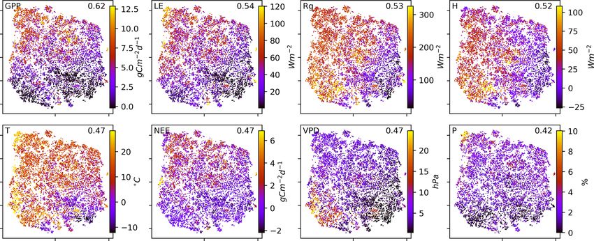
2382 C. Krich et al.: Functional convergence of biosphere–atmosphere interactions
was performed also without this setting, i.e. allowing influ- terpretability of the embedding axes due to the non-linear na-
ences of other variables on Rg . The conclusions we draw are ture and its fairly long computation time for large datasets.
not affected (cf. Fig. B4). Missing data were flagged as such Further, distances between far-separated points and those be-
and are ignored by PCMCI. To avoid effects on the network longing to different clusters in the embedding space are not
structure from gap-filling, we used the following quality flag (necessarily) comparable to the original distances. This is as
thresholds. A daily data point is not used if its quality flag t-SNE does not preserve both the global and local structure
is below 0.6 (i.e. more than 60 % of measured and good- at the same time, which is attempted by UMAP. UMAP was
quality gap-filled data). In the case that more than 25 % of developed as an improvement of t-SNE regarding structure
data points of the 3-month window are flagged as bad qual- preservation and results also in a shorter run time especially
ity, the time window is removed from the analysis. To anal- for higher dimensions. A comparison of t-SNE and UMAP is
yse the factors influencing network structure, we consider the given in Appendix C in McInnes et al. (2018). According to
mean values over the respective time period of the variables Kobak and Linderman (2019), the global structure preserva-
included in the network calculation and additionally those of tion of UMAP is not an inherent characteristic of the method
GPP, P , and SWC. GPP, P , and SWC were not included in itself but rather stems from the chosen initialisation.
the network calculation because certain characteristics can As we are dealing with an unsupervised method, there is
impinge on network estimation. GPP is derived using NEE no obvious measure to assess the quality of an embedding,
and T . Any of the links GPP–T and GPP–NEE thus could be as each method optimises a different error function. A mea-
due to its processing rather than an actual dependence. P , on sure commonly used for the comparison and characterisation
the other hand, typically yields non-intuitive results due to of dimensionality methods is the agreement between K-ary
its binary character (precipitation of a certain amount – zero neighbourhoods (the K nearest points to an observation) in
precipitation), while its effects occur more smoothly (e.g. in- the high-dimensional and low-dimensional space. The mea-
crease in transpiration or respiration), and its strong deviation sure RNX (K) (Lee et al., 2015) gives a measure of the im-
is from a normal distribution. Further, it can happen that over provement of the embedding of K-ary neighbourhoods over
the time period of network estimation no precipitation oc- random embeddings. For an embedding with random coor-
curs, rendering such periods not analysable. The issue with dinates we obtain RNX (K) ≈ 0, and if the K-ary neighbour-
SWC is its lower availability, and for those sites that have hoods are perfectly preserved we obtain RNX (K) = 1. As
such measurements it might be applied at a differing depth. this measure depends on the neighbourhood size K, we can
The depth that is mostly present is at shallow depths of 5 or draw a curve over K that characterises if the method is better
10 cm. The upper soil layer, however, dries out quickly and at maintaining global or local neighbourhoods. The area un-
can explain only little of the latent heat flux. der the RNX (K) curve gives an idea of the overall quality of
the embedding. An intercomparison of the three dimension-
2.4 Dimensionality reduction ality reduction methods using this measure shows t-SNE to
perform best (see Figs. B1, B2, and B3).
For the dimensionality reduction, we tested principal compo-
nent analysis (PCA; Pearson, 1901), t-distributed stochas- 2.5 Distance correlation
tic neighbour embedding (t-SNE; Maaten and Hinton,
2008), and uniform manifold approximation and projection Distance correlation (Székely et al., 2007) is a non-linear
(UMAP; McInnes et al., 2018). PCA is the standard method measure to quantify the dependence between two vectors. It
for dimensionality reduction; it is commonly used, linear, has been used successfully to assess the influence of vari-
fast, and easily interpretable regarding the meaning of its ables on the low-dimensional embedding (Kraemer et al.,
axes (the principal components). A PCA embedding typi- 2020b). Székely et al. (2007) details its empirical definition
cally fails to reveal complex clusterings because it main- for a sample (X, Y) = {(Xk , Yk ) : k = 1, . . ., n} with X ∈ Rp
tains large-scale gradients but often produces embeddings in and Y ∈ Rq as follows:
r
which far away points appear very close in the embedding. Vn2 (X,Y)
, Vn2 (X, X)Vn2 (Y, Y) > 0,
In contrast t-SNE aims to preserve local neighbourhoods. R2n (X, Y) = Vn2 (X,X)Vn2 (Y,Y) (1)
0, Vn2 (X, X)Vn2 (Y, Y) = 0,
Therefore it calculates first similarity scores for each point
pair using Euclidean distances and Gaussian distributions. where Vn2 (X, Y)
Subsequently it randomly projects the data onto the lower- Pis the empirical distance covariance with
Vn2 (X, Y) = n12 nk,l=1 Akl Bkl . Akl and Bkl are distance ma-
dimensional space and attempts to rearrange points in a way trices defined by
that the previously determined similarities are obtained. To
assess the similarities in the low-dimensional space, how- Akl = akl − a k − a l + a,
a = n12 nk,l=1 akl ,
P
ever, it uses a Student t distribution. This helps to separate
a k = n1 nk=1 akl ,
P
points which are also originally separated. This procedure (2)
makes t-SNE very good at visualising clusters in the data a l = n1 nl=1 akl ,
P
and non-linear relationships. Drawbacks are the difficult in- akl = |Xk − Xl |p ,
Biogeosciences, 18, 2379–2404, 2021 https://doi.org/10.5194/bg-18-2379-2021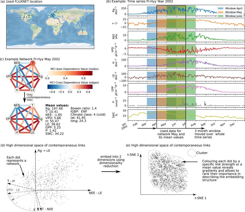
C. Krich et al.: Functional convergence of biosphere–atmosphere interactions                                                   2383

with | · |p resembling the Euclidean norm in Rp .                   our analysis on these 15 links, as they contain most infor-
   Distance correlation can be used to quantify the depen-          mation. This is done by performing the dimensionality re-
dence between two sets of observations of differing dimen-          duction on contemporaneous links and neglecting the lagged
sionality. In our case these two vectors are firstly a link         ones. The rationale of employing a dimensionality reduc-
strength or an underlying quantity of the networks (Fig. 1d)        tion is the following. Each of the estimated networks con-
and secondly the networks’ position in the low-dimensional          stitutes one observation in a high-dimensional space with a
embedding (Fig. 2d). The resulting dependence value is used         network’s links spanning its axes (Fig. 1d). Projecting this
to rank the quantities in their ability to describe the structure   high-dimensional space onto two dimensions (Fig. 1e) allows
of the low-dimensional embedding.                                   first of all for visualisation. In the case that the data consist
                                                                    of a structure that can be “identified” by the dimensional-
2.6   Clustering and median network trajectories                    ity reduction method, the visualisation reveals the dominant
                                                                    features of transitions between different states of biosphere–
On the reduced space we applied a clustering method named           atmosphere interactions. The dominant features are the links
“ordering points to identify the clustering structure” (OP-         that appear with strong gradients in the low-dimensional em-
TICS; Ankerst et al., 1999). OPTICS finds clusters by iden-         bedding. To quantify and later rank the gradients exhibited
tifying regions of high density that contain a certain number       by each link, we use the measure distance correlation (see
of data points (minsamples ). The cluster borders are defined by    Sect. 2.5). Therefore, we calculate the distance correlation of
a certain drop in reachability of further data points (maxeps       the link strengths (Fig. 1d) with their position on the low-
and xi). This allows points that lie outside the reachabil-         dimensional embedding axes (Fig. 2d). We also examine the
ity of neighbouring clusters to remain unclustered. The fol-        distance correlation of secondary quantities with the axes.
lowing settings were used for clustering: min_samples = 80,         The secondary quantities are firstly mean values of variables
max_eps = 8, and xi = 0.5. We calculated mean networks for          calculated for each 3-month period of network estimation
each cluster by calculating the mean MCI value for each             as well as secondly static values like climate class, vegeta-
contemporaneous link among all networks contained in the            tion type, or location. The secondary quantities are used to
cluster and only took those links that had an absolute value        find covariates of the low-dimensional embedding that can
above 0.2.                                                          help to explain its structure. In a next step, we cluster the
                                                                    low-dimensional embedding to further understand to which
2.7   Visualising ecosystem trajectories
                                                                    network structures the gradients of link strength lead (see
As we calculated networks for each month for each measure-          Sect. 2.4) and calculate the cluster’s average networks (a sim-
ment year for each FLUXNET site (if data requirements are           ple mean). Up to this point (Sect. 3.1 and 3.2), we have anal-
fulfilled; see Sect. 2.3), annual trajectories can be visualised    ysed the manifold of biosphere–atmosphere interactions and
in the low-dimensional embedding by connecting the dots             can address the first part of our hypothesis. As each point
representing the monthly networks of a specific year. Fur-          of the low-dimensional embedding represents the biosphere–
ther, for each ecosystem, we calculated a monthly median            atmosphere interactions of a specific ecosystem at a specific
trajectory within the t-SNE space which is composed of its          time, we can investigate the behaviour of specific ecosystems
monthly median networks. To this end, we calculated non-            (see Sect. 2.7). Therefore we look at the monthly median and
intersecting convex hulls which consisted of at least three         annual trajectories of certain ecosystems (Sect. 3.3 and 3.4).
data points (networks within the t-SNE space belonging to           This leads to the answer of the second part of our hypothesis.
the same ecosystem, representing the same month, in at least
3 years). The monthly median network is the average of the
networks lying on (greater than or equal to three networks)         3     Results and discussions
or in the inner hull (less than networks).
                                                                    3.1    Two-dimensional embedding of
2.8   Workflow                                                             biosphere–atmosphere networks

Our restrictions on the data length and quality resulted in         To find the most suitable dimensionality reduction method,
a selection of 119 FLUXNET sites (Fig. 1a). Applying the            we evaluated three different methods (PCA, t-SNE, and
above-described procedure we obtained 10 038 networks for           UMAP) with respect to their ability to project the high-
the different months and sites. An example network esti-            dimensional network space onto two dimensions. To com-
mated by PCMCI is shown in Fig. 1c. The strongest and               pare the low-dimensional embedding spaces, we used the
most consistent links are contemporaneous, indicating that          RNX (K) measure (see Sect. 2.4) which quantifies how well
interactions happen on timescales shorter than the time res-        neighbourhoods are preserved when projecting the high-
olution. While lagged common drivers are excluded, con-             dimensional space onto fewer dimensions. We found that t-
temporaneous links can still be spurious due to contempo-           SNE achieved the best projection, by best preserving both
raneous confounding (see Sect. 2.2). Nevertheless, we focus         local and distant neighbourhoods (cf. Sect. 2.4 and Figs. B1

https://doi.org/10.5194/bg-18-2379-2021                                                    Biogeosciences, 18, 2379–2404, 2021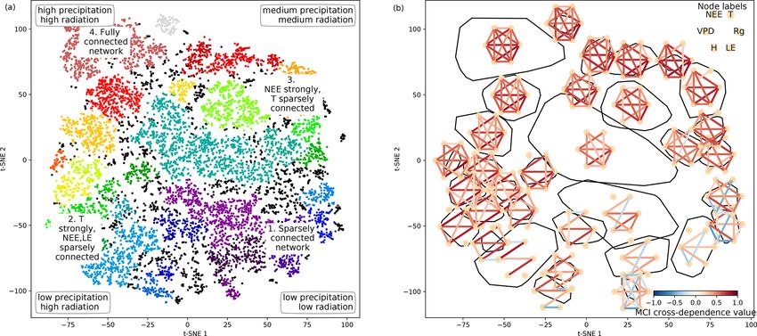
2384                                           C. Krich et al.: Functional convergence of biosphere–atmosphere interactions

Figure 1. Schematic representation of the workflow. (a) Eddy covariance data from the FLUXNET database are selected (119 sites). (b) For
each site we used the time series of global radiation Rg , air temperature T , vapour pressure deficit VPD, net ecosystem exchange NEE,
sensible heat H , latent heat LE, gross primary productivity GPP, precipitation P , and soil water content SWC. Networks are estimated in
3-month moving windows using Rg , T , NEE, VPD, LE, and H . (c) An example interaction network for FI-Hyy (Hyytiälä) in May 2002.
Contemporaneous links are given by straight (undirected) edges; lagged links are given by curved arrows with a number indicating the time
lag. The strongest and most persistent links are contemporaneous. Thus we limit our analysis to those links. (d) Each 3-month network can
be interpreted as an observation in a 15-dimensional space (each contemporaneous link is one dimension). (e) Dimensionality reduction
projects all interaction networks into a two-dimensional space preserving its local-neighbourhood structure. Here any subsequent analysis
and interpretation will be realised.

and B2). This is unexpected, as UMAP is said to intentionally          reveals that the link strengths are ordered along gradients; i.e.
preserve the global structure. Yet, as can be seen in Fig. 4a,         they exhibit some dependence with the t-SNE axes. Using
the networks almost form a continuum. Thus, by maintaining             distance correlation to rank those gradients (see Sect. 2.5),
the local-neighbourhood structure, also the global structure is        we find the links NEE–LE (R = 0.75), Rg –LE (R = 0.73),
preserved within t-SNE.                                                and T –H (R = 0.69) to have the strongest gradients. The
   The two-dimensional embedding by t-SNE of biosphere–                connection between carbon and water fluxes as well as the
atmosphere interactions is ordered primarily by dependen-              role of energy input to sustain water fluxes (if available in
cies including carbon flux (NEE) and energy distributions              the soil) are well-known and investigated dependencies (Beer
(LE and H ). This can be seen in Fig. 2, which shows the               et al., 2010; Luyssaert et al., 2007).
Fig. 2d embedding colour-coded by the strength of individ-                To search for covariates that help to explain – and if
ual links, i.e. MCI partial-correlation values. The colouring          thought further, help to predict the network structures – we

Biogeosciences, 18, 2379–2404, 2021                                                       https://doi.org/10.5194/bg-18-2379-2021
C. Krich et al.: Functional convergence of biosphere–atmosphere interactions                                                           2385

Figure 2. Two-dimensional embedding of 3-monthly biosphere–atmosphere networks realised via t-SNE. Shown is the distribution of link
strengths among the networks. The strength is estimated via MCI partial-correlation values. Panels are sorted by the distance correlation of
the link’s MCI value with the axes (value in the upper-right corner). As Rg is set as a potential driver (PCMCI parameter selected_links; see
Table A2), connections including Rg are directed →. This setting does not affect the results (see Fig. B4).

colour-coded the embedding by the networks’ underlying                   3.2   Clusters of characteristic ecosystem–atmosphere
mean conditions, i.e. the average over the respective time                     networks
window, of the exchange rates (GPP, NEE, LE, and H ) as
well as meteorological conditions (Rg , T , VPD, and P ).                As we apply a significance threshold to each link of the
This is shown in Fig. 3. Clearly, the mean exchange rates                estimated network structures (see Sect. 2.3), the networks
and meteorological conditions – although not considered in               typically lack weak links. This leads to a certain degree of
the estimation of the networks – are related to the observed             clustering among the networks, which we identified using
biosphere–atmosphere interactions. On the contrary, corre-               the OPTICS approach (see Sect. 2.6; Ankerst et al., 1999)
sponding vegetation types and Köppen-Geiger classes are                  (Fig. 4a). Cluster boundaries are shown by the convex hulls
not as much related as displayed in Fig. B6 in the Appendix              in Fig. 4b, where we also visualise the mean networks of each
. The results show that a high-dimensional space encom-                  cluster. This visualisation reveals that the mean networks of
passing more than 10 000 ecosystem networks representing                 the clusters situated at the embedding’s edges can be re-
the states of biosphere–atmosphere interactions from ecosys-             garded as archetypes of network structures, i.e. extremal,
tems of various geographic origins can be reduced to a com-              characteristic states (similar to the concept of endmember
pact two-dimensional manifold characterised by four edges                states). The four states can be described as follows:
and gradients of mean biosphere and atmosphere conditions.                  – Type 1 is a sparsely connected network. Links, if
While gradients in MCI partial-correlation strength are ex-                   present, are very weak and predominantly exist among
pected, as they were used as features in the dimensionality                   atmospheric variables. Mean atmospheric conditions
reduction, gradients in mean climatic and biospheric condi-                   are characterised by low energy input (low Rg and T ).
tions were not. This information thus must be entailed in the                 Carbon and water fluxes are consequently close to 0,
networks’ structure. To better grasp the distribution of net-                 and daily averages of sensible heat can even reach nega-
work structures, we further analyse the emerging clusters.                    tive values. Such conditions reflect high-latitude ecosys-
                                                                              tem winter states experienced by ecosystems like the ev-
                                                                              ergreen needleleaf forest (ENF) of Finland, i.e. Hyytiälä
                                                                              (FI-Hyy) and Sodankylä (FI-Sod), and Canada, i.e. the
                                                                              UCI-1850 burn site (CA-NS1) and the Quebec – Eastern
                                                                              Boreal (CA-Qcu) site during December and January.

https://doi.org/10.5194/bg-18-2379-2021                                                           Biogeosciences, 18, 2379–2404, 2021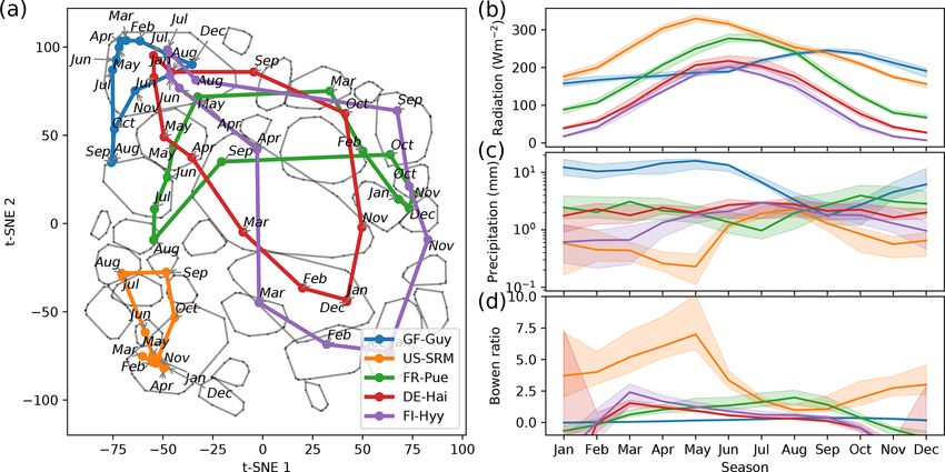
2386 C. Krich et al.: Functional convergence of biosphere–atmosphere interactions
Figure 3. Two-dimensional embedding coloured by underlying mean exchange rates and meteorological conditions. The mean values are
calculated over the respective time periods used for the network estimation. Each network is estimated on a 3-month window of daily time
series data. Values are cut off at the highest and lowest percentile. Distance correlation of the shown quantity with the axes is given in the
upper-right corner of each panel.
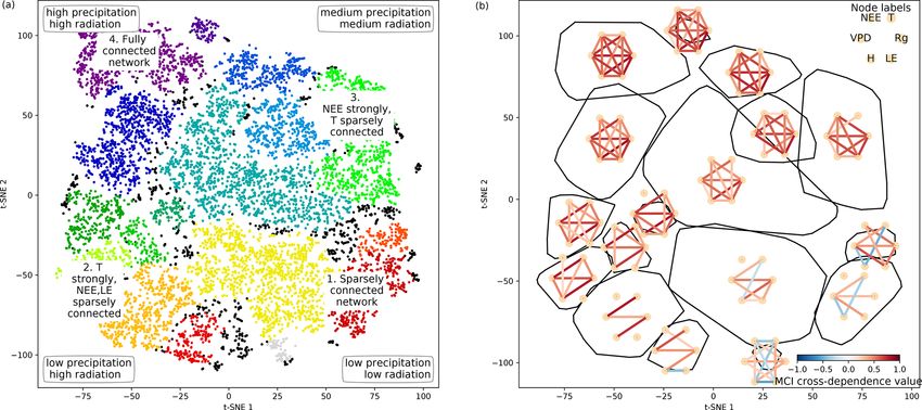
Figure 4. Structure of the two-dimensional embedding. (a) t-SNE space clustered by the OPTICS approach (Ankerst et al., 1999). Colours
represent different clusters; black dots are not attributed to a cluster. Indicated are the four archetypes of network connectivity and the
networks’ underlying meteorological conditions. (b) Convex hulls of clusters and their average network, i.e. average over all networks
belonging to one cluster. Average networks are thresholded at a minimum link strength of 0.2. A finer clustering can be found in Fig. B5 in
the Appendix.
– Type 2 consists of strong links among atmospheric vari- woody-savanna (WSA) Santa Rita Mesquite (US-SRM)
ables, but LE and NEE are weakly, not, or even neg- as well as the grassland Santa Rita (US-SRG) sites,
atively connected to the atmosphere, i.e. the meteoro- Audubon Research Ranch (US-Aud), and Sturt Plains
logical variables. This network structure coincides with (AU-Stp) during the dry season.
high energy input (high Rg and T ) but low water avail-
ability (low P and SWC and high VPD). A high Bowen – Type 3 exhibits the same strong links among Rg , VPD,
ratio, i.e. the ratio between sensible heat and latent heat, and H as Type 2, but T is weakly or not connected.
representing aridity, and low absolute carbon fluxes The opposite is true for links of LE and NEE, which are
(GPP and NEE) are the consequence. These conditions strongly connected to the other variables (except T ). Rg
are typically present at semi-arid ecosystems like the and T are considerably lower than in Type 2 (approx-
Biogeosciences, 18, 2379–2404, 2021 https://doi.org/10.5194/bg-18-2379-2021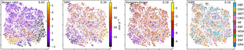
C. Krich et al.: Functional convergence of biosphere–atmosphere interactions                                               2387

     imately by 100 W m−2 and 10 ◦ C), but because of suf-         variety of land-surface processes can be largely summarised
     ficient water availability the Bowen ratio is between 0       by on the one hand productivity measures and on the other
     and 1. Typical ecosystems in this state are mid- to high-     hand water and energy availability. Both water and energy
     latitude forests during spring or autumn, e.g. Harvard        availability need to be high for highly productive states, yet
     Forest EMS Tower (US-Ha1, deciduous broadleaf for-            the lack of either of them leads to low productivity (Kraemer
     est (DBF)), Roccarespampani 1 (IT-Ro1, DBF), Viel-            et al., 2020a). This biosphere state triangle is found in our
     salm (BE-Vie, mixed forest (MF)), and Hyytiälä (FI-           analysis by the network types 1 (cold – low connectivity), 2
     Hyy, ENF).                                                    (dry – NEE/LE weakly connected), and 4 (high productiv-
                                                                   ity – fully connected). Yet, a fourth network type (type 3) is
  – Type 4 is fully and strongly connected. Both energy in-
                                                                   naturally occurring in the t-SNE space, as we here include
    put and water availability are high, leading to Bowen
                                                                   interactions with the atmosphere.
    ratios around 1. This network state is typically present
                                                                      Up to this point we have found strong evidence supporting
    in tropical forests like the Guyaflux site in French
                                                                   our first hypothesis. The manifold of biosphere–atmosphere
    Guiana (GF-Guy) (evergreen broadleaf forest (EBF))
                                                                   interactions can be represented rather well by two dimen-
    but can temporarily be also reached by a variety of
                                                                   sions, which we identified to be most consistent with en-
    other ecosystems, e.g. mid- and high-latitude forests
                                                                   ergy and water availabilities. It is confined by four char-
    like Hainich (DE-Hai, DBF), Tharandt (DE-Tha, ENF),
                                                                   acteristic states and populated homogeneously by the ob-
    BE-Vie (MF), and FI-Hyy (ENF) as well as woody sa-
                                                                   served network states. Having an understanding of the low-
    vanna (WSA) such as Howard Springs (AU-How) and
                                                                   dimensional embedding’s structure now allows us to analyse
    grassland (GRA) such as Daly River Savanna (AU-
                                                                   specific ecosystem behaviour.
    Dap).
The archetypes of networks are located at the edges of the         3.3   Ecosystems’ median trajectories
two-dimensional space and thus could define two imaginary
axes. From a physical point of view, energy is required for        Each point in the reduced t-SNE space represents a
each process and interaction to occur, e.g. photosynthesis         biosphere–atmosphere interaction network for a given month
or evaporation (Bonan, 2015). Therefore, transitions along         and ecosystem. Hence, we can trace an ecosystem’s tra-
the axis connecting the network types 1 and 4 might be in-         jectory through time. We are first focusing on an ecosys-
terpreted as energy controlled, as dependencies among all          tem’s median monthly trajectory (see Sect. 2.7) within the
variables fade or increase consistently. Transitions along the     low-dimensional space. We can see that the median trajec-
axis connecting network types 2 and 3 are explainable by           tories reflect seasonal patterns of meteorological conditions
a combination of water availability and a temperature gra-         (Fig. 5). For example, mid-latitude sites like FR-Pue (Puech-
dient. Low water availability but high temperatures cause a        abon, EBF), DE-Hai (DBF), and FI-Hyy (ENF) exhibit a
shutdown of stomatal conductance or ecosystems to enter a          strong seasonal variation of Rg and span a long distance in
dormant state, which leads to low carbon and water fluxes          the t-SNE space. In contrast, tropical ecosystems like GF-
and low connectivity. On the other hand, sufficient water and      Guy (EBF) constantly have high Rg and exhibit predomi-
medium temperatures (around the optimum of photosynthe-            nantly network type 4, indicative of highly productive condi-
sis) allow for carbon and water fluxes but reduce the influ-       tions, while DE-Hai or FI-Hyy reach this connectivity pattern
ence of varying temperatures, leading to connected NEE and         only during peak growing season. US-SRM (WSA), how-
LE but disconnected T . And indeed these patterns and gradi-       ever, has similar or even higher Rg values throughout the
ents exist. Mean Rg is lowest at network type 1 and almost         year but barely manages to deviate from type 2, which is
linearly increases towards network type 4. P is lowest at net-     in accordance with its low water availability. The amount
work types 1 and 2. In combination with high energy input          of precipitation further aligns with differences and charac-
network type 2 has the lowest SWC values and the highest           teristics of the trajectories of FR-Pue, DE-Hai, and FI-Hyy.
Bowen ratios (see Appendix Fig. B6). SWC is higher but             For example, FI-Hyy shows some deviation towards edge 2
quite dispersed elsewhere, suggesting that at a certain point      in February and March, as does FR-Pue in June, July, and
water limitations are fading out. T values of course also show     August. For both, mean precipitation is lowest during these
an increase not only from network types 1 to 4 (as radiation)      months. These behaviours demonstrate what the previous
but also from network types 3 to 2 and are actually rather low     figures (Figs. 3 and 4) have already suggested: ecosystems
(8 to 15 ◦ C) at network type 3 (see Fig. 3). As meteorological    populate the low-dimensional space and migrate within as
conditions affect biosphere productivity, network types 1 and      allowed by their climatic conditions. Thereby they can ex-
2 exhibit low, type 3 medium, and type 4 high productivity,        hibit a wide range of interaction structures as can be seen
i.e. estimated as GPP. In short, the clustering revealed that      from the mid-latitude sites. As these behaviours are multi-
changes in energy and water availability can explain major         year averages, they could resemble more ecosystem adapta-
transitions between different states of biosphere–atmosphere       tion to median climatic conditions than flexible adjustment
interactions. This is in line with a recent study showing that a   of biosphere–atmosphere interactions to quickly changing

https://doi.org/10.5194/bg-18-2379-2021                                                  Biogeosciences, 18, 2379–2404, 2021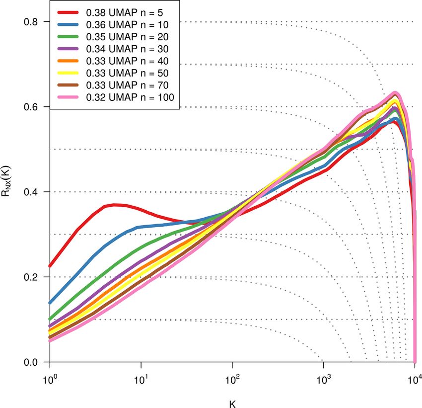
2388 C. Krich et al.: Functional convergence of biosphere–atmosphere interactions
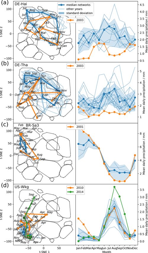
Figure 5. Median trajectories of selected sites (a) and their corresponding mean values of radiation, precipitation, and the Bowen ratio (b).
In winter months the Bowen ratio can turn negative. Nevertheless we set the lower limit of the y axis to 0. As networks are calculated using
a centred 3-month moving window, each month is ascribed to a network. Thus, the behaviour of an ecosystem can be tracked by its monthly
networks, which form trajectories for each year. An ecosystem’s monthly median trajectory is composed of the two-dimensional monthly
median networks (see Sect. 2.7 for details).
meteorological conditions. If biosphere–atmosphere interac- The network structure of US-Wkg becomes fully connected
tions are confined by adaptation shall be investigated in the (network type 4) in September 2014 with above-average pre-
final analysis section. cipitation (NOAA, 2015) (Fig. 6d). In summary, climatic
extremes are visible in an ecosystem’s trajectory as strong
3.4 Deviations from ecosystem median trajectories deviations from the median trajectory. With this finding we
have to reject our second hypothesis that owing to an ecosys-
The remaining open question is how flexibly do the networks tem’s adaptation its accessible functional states are limited to
adjust to deviations from mean climatic conditions. There- a certain range. The opposite seems to be valid. Biosphere–
fore, we look at climatic anomalies. Figure 6 shows the tra- atmosphere interactions can flexibly follow atmospheric con-
jectories of ecosystems during anomalous dry or wet condi- ditions and are not confined to certain states.
tions. During the European heatwave of 2003, in July and
August the trajectories of two temperate central European 3.5 Functional convergence of biosphere–atmosphere
forests, DE-Hai and DE-Tha, no longer manage to estab- interactions
lish a network structure resembling network type 4, typical
for these ecosystems during their highly productive phase. We have seen that networks representing biosphere–
Instead they are shifted towards network type 2, associated atmosphere interactions strongly align with prevailing mean
with drier conditions (Fig. 6a and b). Similarly, the ecosys- meteorological conditions. Moreover, the visualisation of
tem BR-Sa3 (EBF) in the Brazilian tropical rainforest shows ecosystem trajectories within the t-SNE space (Figs. 5 and 6)
substantial deviations towards network type 2 during the ex- and the distributions of vegetation types and climatic regions
ceptional dry season of 2001 (August, September, and Oc- (Appendix Fig. B6) reveal that ecosystems across vegeta-
tober) (Marengo et al., 2018) (Fig. 6c). In contrast, US- tion types and climatic regions can exhibit similar biosphere–
Wkg (Walnut Gulch Kendall Grasslands) is a grassland ac- atmosphere interactions if their meteorological conditions
customed to dry conditions and thus predominantly exhibits are similar. For example, we found a fully connected network
low water and carbon fluxes resulting in network structures (type 4) to be associated with high radiation and water avail-
like those of network type 2; i.e. water and carbon fluxes ability and thus optimal growing conditions, which results in
are barely or even not connected. Carbon and water fluxes high carbon and water fluxes. Diverging from optimal grow-
of semi-arid ecosystems, however, are known to respond ing conditions, links in the networks weaken and disappear.
quickly and strongly to sufficient precipitation (Potts et al., This behaviour can be understood as the functional conver-
2019; Leon et al., 2014; Reynolds et al., 2004). This sensi- gence of ecosystems, which corroborates the hypothesis that
tivity is found to carry over to the network structure as well. ecosystems have a low number of key processes that deter-
Biogeosciences, 18, 2379–2404, 2021 https://doi.org/10.5194/bg-18-2379-2021C. Krich et al.: Functional convergence of biosphere–atmosphere interactions 2389
dominated by changes in biosphere connectivity, i.e. LE and
NEE.
In fact, the dominance of climatic drivers in controlling the
temporal evolution of ecosystem functioning emerges also
in other studies (Musavi et al., 2017; Schwalm et al., 2017;
Kraemer et al., 2020a), as they showed that carbon fluxes are
primarily controlled by climatic factors. Yet, these and others
also show the role of biotic factors in shaping the responses
of ecosystem processes to climatic variability. For example,
Musavi et al. (2017) revealed in a global ecosystem study
that species diversity and ecosystem age decrease interan-
nual variability of GPP. Similarly, Wagg et al. (2017) showed
biodiversity to increase long-term stability of ecosystem pro-
ductivity. In regional studies Wales et al. (2020) found the
stability of net primary production to be affected by the kind
and severity of disturbances. Tamrakar et al. (2018) showed
that seasonal carbon fluxes were more sensitive to environ-
mental conditions in a homogeneous forest compared to a
heterogeneous one. It would be of interest to investigate to
which degree the effects of biotic factors also translates to
the sensitivity of the network structure.
Furthermore, extreme heat and drought events (Sippel
et al., 2018) or compound events in general (Zscheischler
et al., 2020) can severely disrupt ecosystem functions. The
time of recovery from such disturbances is a crucial parame-
ter in assessing ecosystem resilience. Schwalm et al. (2017)
showed that the recovery time measured, as the recovery in
GPP is primarily influenced by climate but secondarily by
biodiversity and CO2 fertilisation. Assessing the recovery
time via GPP already puts the ecosystem functioning into
focus. The presented framework here, i.e. the sensitivity of
an ecosystem’s network structure to meteorological condi-
tions, might be a valuable asset in studying reaction time and
strength to and recovery from extreme events, as it not only
utilises one variable but also the interactions of a set of vari-
Figure 6. Abnormal conditions in meteorological conditions (here ables, thereby capturing more comprehensively an ecosys-
precipitation) become visible in an ecosystem’s trajectory. (a) Tra- tem state. A drawback is the reduced temporal resolution
jectories within the low-dimensional space of the ecosystems (a certain time period of daily or even half-hourly measure-
Hainich (DE-Hai, DBF), Tharandt (DE-Tha, ENF), Santarem- ments is aggregated to one network), which can be offset by
Km83-Logged Forest (BR-Sa3, EBF), and Walnut Gulch Kendall the moving window approach used here to a certain degree.
Grasslands (US-Wkg, GRA); (b) 3-monthly average of daily pre- Especially with regard to climatic extreme conditions in re-
cipitation data. cent years with observed vegetation dieback in, for exam-
ple, DE-Hai (Schuldt et al., 2020), further studies could also
shed light on the role of adaptation in shaping biosphere–
mine ecosystem behaviour (Lambert, 2006; Meinzer, 2003; atmosphere interactions. Our study suggests that adaptation
Shaver et al., 2007), rendering their behaviour transparent to a lesser degree limits the range of possible interactions
and predictable. but enables sustaining and persisting certain conditions for
Criticism might rise, as the larger part of the biosphere– longer periods. The focus of further studies thus could be to
atmosphere interaction network indeed is a pure atmospheric elucidate the role of biotic factors in influencing ecosystem
network, i.e. Rg , T , VPD, and H . Thus strong associations of trajectories as well as the role of adaptation and the response
networks and their trajectories with atmospheric conditions to extreme events.
could be dominated by changes in this atmospheric network.
Figure 2, however, suggests the opposite. The strongest gra-
dients are given by the links NEE–LE and Rg –LE, and tran-
sitions along the axis connecting types 2 and 3 (cf. Fig. 4) are
https://doi.org/10.5194/bg-18-2379-2021 Biogeosciences, 18, 2379–2404, 20212390 C. Krich et al.: Functional convergence of biosphere–atmosphere interactions
3.6 Limitations of the study vegetation type and climatic region. Such behaviour is strong
evidence for functional convergence of ecosystems; i.e. their
Finally, we would like to take a critical view on our analysis behaviour is determined by a low number of key processes.
approach. As stated in Sect. 2.2, PCMCI might fail to iden- For further studies, we suggest focusing on the role of biotic
tify some spurious links due to the occurrence of contempo- factors such as, for example, plant functional types, ecosys-
raneous confounders. Thus networks can not be interpreted tem age, and adaptation. These factors could play a crucial
causally, but this does not severely hinder their value for the role in understanding the ecosystem coping strategies to cli-
current analysis. In addition we include a rather limited set of matic extremes.
variables into the network estimation. Thus we cannot and do
not claim that ecosystems become fully alike under similar
meteorological conditions. Yet, on the timescale investigated
the data show that the interactions among the chosen set of
variables can be described by very similar structures. Follow-
up studies might search for and include further biosphere
variables. Currently, an analysis of the biotic effects on the
network structure is hampered because the t-SNE space is
not metric. Thus, for instance, the effect of a drought with
a similar magnitude in a boreal and temperate forest cannot
simply be compared by the deviation from their median tra-
jectory.
4 Conclusions
We analysed the functional behaviour of a variety of ecosys-
tems using the FLUXNET database of carbon, water, and en-
ergy flux measurements. In particular, we examined the in-
teraction structure between biosphere–atmosphere fluxes as
well as atmospheric state variables using PCMCI, a method
to estimate causal relationships from empirical time series
under certain assumptions. Using non-linear dimensionality
reduction, we find evidence supporting our hypothesis that
the manifold of existing states is bound by few, i.e. four,
archetypes of network states. They are characterised on the
one hand by a fully connected and almost unconnected net-
work structure and on the other hand by an antagonistic cou-
pling of carbon and water flux with temperature – when
one is strongly coupled, the other is decoupled. The transi-
tions between these states correlate well with gradients of
meteorological drivers, i.e. radiation and water availability.
The movement of an ecosystem within that space therefore
strongly aligns with changes in meteorological conditions.
This, however, also leads to similar behaviour under similar
conditions for strongly contrasting ecosystems. For example,
forests of mid or even high latitudes exhibit an interaction
structure similar to tropical forests given high radiation and
water availability during summer. Yet, this state can also be
reached by predominantly dry ecosystems like steppe grass-
lands given sufficient precipitation. In contrast if productive
ecosystems are struck by a severe drought, like central Eu-
ropean ecosystems in 2003, the behaviour can adapt more to
that of a Mediterranean ecosystem. Thus the second part of
our hypothesis must be rejected. The analysis shows that the
biosphere–atmosphere interaction structure can adapt flexi-
bly to prevailing conditions and is widely independent of
Biogeosciences, 18, 2379–2404, 2021 https://doi.org/10.5194/bg-18-2379-2021C. Krich et al.: Functional convergence of biosphere–atmosphere interactions 2391
Appendix A: Methods
Table A1. List of FLUXNET sites used for the generation of artificial datasets and the time period used. IGBP: International Geosphere–
Biosphere Programme. DBF: deciduous broadleaf forest; OSH: open shrubland; WET: wetland; CRO: cropland; CSH: closed shrubland; MF:
mixed forest; EBF: evergreen broadleaf forest; WSA: woody savanna; SAV: savanna; ENF: evergreen needleleaf forest; GRA: grassland.
FLUXNET ID IGBP Köppen–Geiger Start year End year Data reference
class
AT-Neu GRA Dfb 2002 2012 Wohlfahrt et al. (2008)
AU-ASM ENF BSh 2010 2014 Cleverly et al. (2013)
AU-Cpr SAV Csa 2010 2014 Meyer et al. (2015)
AU-DaP GRA Aw 2007 2013 Beringer et al. (2011a)
AU-DaS SAV Aw 2008 2014 Hutley et al. (2011)
AU-Dry SAV 2008 2014 Cernusak et al. (2011)
AU-How WSA Aw 2001 2014 Beringer et al. (2007)
AU-Stp GRA Aw 2008 2014 Beringer et al. (2011b)
AU-Tum EBF Cfb 2001 2014 Leuning et al. (2005)
AU-Wom EBF Cfb 2010 2014 Arndt et al. (2021)
BE-Bra MF Cfb 1996 2014 Carrara et al. (2004)
BE-Lon CRO BSk 2004 2014 Moureaux et al. (2006)
BE-Vie MF Cfb 1996 2014 Aubinet et al. (2001)
BR-Sa3 EBF 2000 2004 Saleska et al. (2003)
CA-Mer WET Dwb 1998 2005 Lafleur et al. (2003)
CA-NS1 ENF BWk 2001 2005 Goulden et al. (2006)
CA-NS2 ENF BWk 2001 2005 Bond-Lamberty et al. (2004)
CA-NS3 ENF 2001 2005 Wang et al. (2002a)
CA-NS5 ENF BSk 2001 2005 Wang et al. (2002b)
CA-NS6 OSH BSk 2001 2005 Wang et al. (2002c)
CA-Qcu ENF Dwb 2001 2006 Giasson et al. (2006)
CA-Qfo ENF Dfb 2003 2010 Chen et al. (2006)
CA-SF2 ENF BSk 2001 2005 Rayment and Jarvis (1999a)
CA-SF3 OSH Dwc 2001 2006 Rayment and Jarvis (1999b)
CH-Cha GRA Cfb 2005 2014 Merbold et al. (2014)
CH-Dav ENF Dfc 1997 2014 Zielis et al. (2014)
CH-Fru GRA Dfb 2005 2014 Imer et al. (2013)
CH-Lae MF BWk 2004 2014 Etzold et al. (2011)
CH-Oe1 GRA Cfb 2002 2008 Ammann et al. (2009)
CH-Oe2 CRO BSk 2004 2014 Dietiker et al. (2010)
CZ-BK1 ENF Dwb 2004 2014 Acosta et al. (2013)
CZ-BK2 GRA Dfb 2004 2012 Sigut et al. (2021)
CZ-wet WET Dfb 2006 2014 Dušek et al. (2012)
DE-Akm WET BWk 2009 2014 Bernhofer et al. (2021a)
DE-Geb CRO Cfb 2001 2014 Anthoni et al. (2004b)
DE-Gri GRA Dfb 2004 2014 Prescher et al. (2010a)
DE-Hai DBF Cfb 2000 2012 Knohl et al. (2003)
DE-Kli CRO Dfb 2004 2014 Prescher et al. (2010b)
DE-Lkb ENF Dwb 2009 2013 Lindauer et al. (2014)
DE-Obe ENF Dfb 2008 2014 Bernhofer et al. (2021b)
DE-Spw WET BWk 2010 2014 Bernhofer et al. (2021c)
DE-Tha ENF Dfb 1996 2014 Grünwald and Bernhofer (2007)
DE-Wet ENF Dfb 2002 2006 Anthoni et al. (2004a)
DK-NuF WET Dfc 2008 2014 Westergaard-Nielsen et al. (2013)
DK-Sor DBF Cfb 1996 2014 Pilegaard et al. (2011)
DK-ZaH GRA ET 2000 2014 Lund et al. (2012)
ES-ES1 ENF BSk 1999 2006 Sanz et al. (2004)
FI-Hyy ENF Dfb 1996 2014 Suni et al. (2003)
https://doi.org/10.5194/bg-18-2379-2021 Biogeosciences, 18, 2379–2404, 2021You can also read