Technical note: Hydrology modelling R packages - a unified analysis of models and practicalities from a user perspective - HESS
←
→
Page content transcription
If your browser does not render page correctly, please read the page content below
Hydrol. Earth Syst. Sci., 25, 3937–3973, 2021
https://doi.org/10.5194/hess-25-3937-2021
© Author(s) 2021. This work is distributed under
the Creative Commons Attribution 4.0 License.

Technical note: Hydrology modelling R packages – a unified analysis
of models and practicalities from a user perspective
Paul C. Astagneau1,2 , Guillaume Thirel1 , Olivier Delaigue1 , Joseph H. A. Guillaume3 , Juraj Parajka4 ,
Claudia C. Brauer5 , Alberto Viglione6 , Wouter Buytaert7 , and Keith J. Beven8
1 Université  Paris-Saclay, INRAE, HYCAR Research Unit, Antony, France
2 Sorbonne   Université, Paris, France
3 Institute for Water Futures and Fenner School of Environment & Society,

Australian National University, Canberra, Australia
4 Institute of Hydraulic and Water Resources Engineering, TU Vienna, Vienna, Austria
5 Hydrology and Quantitative Water Management Group, Wageningen University and Research, Wageningen, the Netherlands
6 Department of Environment, Land and Infrastructure Engineering, Politecnico di Torino, Turin, Italy
7 Department of Civil and Environmental Engineering, Imperial College London, London, UK
8 Lancaster Environment Centre, Lancaster University, Lancaster, UK

Correspondence: Paul C. Astagneau (paul.astagneau@inrae.fr)

Received: 25 September 2020 – Discussion started: 17 October 2020
Revised: 10 March 2021 – Accepted: 5 June 2021 – Published: 8 July 2021

Abstract. Following the rise of R as a scientific program-       of which packages could/should be used depending on the
ming language, the increasing requirement for more trans-        problem at hand. In this regard, the technical features, docu-
ferable research and the growth of data availability in hy-      mentation, R implementations and computational times were
drology, R packages containing hydrological models are be-       investigated. Moreover, by providing a framework for pack-
coming more and more available as an open-source resource        age comparison, this study is a step forward towards sup-
to hydrologists. Corresponding to the core of the hydrolog-      porting more transferable and reusable methods and results
ical studies workflow, their value is increasingly meaning-      for hydrological modelling in R.
ful regarding the reliability of methods and results. Despite
package and model distinctiveness, no study has ever pro-
vided a comparison of R packages for conceptual rainfall–
runoff modelling from a user perspective by contrasting their    1   Introduction
philosophy, model characteristics and ease of use. We have
selected eight packages based on our ability to consistently     Since the early 1960s, many hydrologists have been design-
run their models on simple hydrology modelling examples.         ing models to better understand water cycle processes con-
We have uniformly analysed the exact structure of seven of       trolling river flows (e.g. Todini, 2011; Beven, 2012). These
the hydrological models integrated into these R packages in      models have enabled advances with respect to a wide vari-
terms of conceptual storages and fluxes, spatial discretisa-     ety of applications in hydrology, such as flood forecasting,
tion, data requirements and output provided. The analysis        climate change impact assessment and water resources man-
showed that very different modelling choices are associated      agement. The processes involved in the motion of water at
with these packages, which emphasises various hydrological       the catchment scale are complex (e.g. Wagener et al., 2010),
concepts. These specificities are not always sufficiently well   mainly due to the heterogeneity and nonlinearity of the phys-
explained by the package documentation. Therefore a syn-         ical properties involved. Hydrological modelling can, there-
thesis of the package functionalities was performed from a       fore, be of great use regarding many scientific challenges, as
user perspective. This synthesis helps to inform the selection   it relies on a threefold simplification of time, space and hy-
                                                                 drological processes to either match the average behaviour of

Published by Copernicus Publications on behalf of the European Geosciences Union.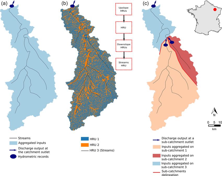
3938                                                P. C. Astagneau et al.: Technical note: Hydrology modelling R packages

the water cycle (Singh et al., 2017) or focus on flow extremes     tant with the increasing development of open-source models,
(e.g. floods, Georgakakos, 2006, and Rozalis et al., 2010, or      there has never been any comparison of hydrological mod-
low flows, Staudinger et al., 2011, and Nicolle et al., 2014).     elling R packages. Such a comparison is required to improve
   Various types of hydrological models exist, which differ        the usability of hydrological models included in the R en-
according to their assumptions on the representation of nat-       vironment. Comparison is a step towards overcoming repro-
ural processes and space and time dependencies (e.g. Clark         ducibility issues related to modelling in computational hy-
et al., 2011, 2017; Beven, 2012). Various programming lan-         drology (Ceola et al., 2015; Hutton et al., 2016; Melsen et al.,
guages enable the use of these hydrological models. For ex-        2017). Furthermore, in addition to the struggle associated
ample, some models are implemented in Python (e.g. EXP-            with a large number of hydrological models and the diffi-
HYDRO hydrological model; Patil and Stieglitz, 2014) or in         culty in finding appropriate bases for model selection (Clark
MATLAB with the MARRMoT toolbox (Knoben et al., 2019).             et al., 2011; Beven, 2012), there are many R packages re-
A significant number of models like MIKE SHE (Danish Hy-           lated to hydrological modelling, making it even harder to se-
draulic Institute, 2017) can only be operated through com-         lect the model best suited for a specific case. Catching the
mercial software and platforms.                                    modelling philosophy (Hrachowitz and Clark, 2017) or dif-
   A large number of models can be found on the R plat-            ferences in a perceptual model (Wrede et al., 2015) behind
form. The R language (R Core Team, 2020a) is an open-              the packages, as well as the technical features offered by
source interpreted language. It was originally designed for        a package, therefore appears to be relevant to hydrologists,
statistics (as an open-source implementation of the S lan-         whether it aims at improving the reliability of intercompar-
guage; Becker et al., 1988) but has since been employed            isons or simply at correctly selecting a model. By referring
in many other scientific fields. The functionalities of the        to the provided documentation, any user should be able to
R language can be extended by packages, some of which in-          make a choice and use a model in full knowledge of its char-
clude features related to hydrology topics. There is a grow-       acteristics, thus guaranteeing good practices (Jakeman et al.,
ing community of users and a large range of documenta-             2006). Unfortunately, despite the wish to standardise pack-
tion, tutorials, manuals and online discussion platforms that      age documentation, especially regarding the rules imposed
have been developed by the R-Hydro community, such as the          by the main R packages repository, the Comprehensive R
CRAN Hydrology Task View on hydrological data and mod-             Archive Network (CRAN; https://cran.r-project.org/, last ac-
elling (https://cran.r-project.org/web/views/Hydrology.html,       cess: 1 March 2021), it remains complicated and sometimes
last access: 1 March 2021) or the page related to R on the         even daunting to select a package among the R packages con-
AboutHydrology blog (https://abouthydrology.blogspot.com,          taining hydrological models. Yet, to our knowledge, there has
last access: 1 March 2021). In addition, many short courses        never been a published study dealing with the comparison of
and workshops are regularly organised (e.g. the “Using R           hydrological modelling R packages. This work should (i) en-
in Hydrology” short course at the European Geosciences             able any newcomer in hydrology, or even more experienced
Union (EGU) General Assembly). The R-Hydro commu-                  hydrologist, to knowledgeably employ one of the packages
nity is also very active in many R projects and websites,          presented in this comparison and (ii) highlight possible im-
such as the rOpenSci project (https://ropensci.org, last ac-       provements for future developments of the packages.
cess: 1 March 2021) or the many code examples available               The review paper published in the Hydrology and Earth
on Stack Overflow (https://stackoverflow.com, last access:         System Sciences journal by Slater et al. (2019) on the place
1 March 2021). R can be used at each step required for a ba-       of R in Hydrology has reached a large part of the hydrolog-
sic study in hydrology (the hydrological workflow steps, see       ical science community. Our work follows on from this re-
Fig. 3 of Slater et al., 2019, that shows the growth of avail-     view and aims at reaching a large portion of hydrological
able packages over the last 10 years). Consequently, there has     modellers within the R-Hydro community, from beginners
been an important increase in the growth and use of hydro-         to highly skilled developers. The objective of this paper is
logical R packages (see Fig. 1 of Slater et al., 2019). Some       to review the pros and cons of using hydrological models
of these packages are designed for hydrological modelling.         implemented within packages in the R environment and to
In this study, we will restrict ourselves to the hydrological      compare and evaluate their applicability and usability. It is
models that are available within the R environment.                not the intention to describe new hydrological model devel-
   At a time when data management is a key issue in many           opments or evaluate the models. We present the package se-
branches of science, R has taken a central place in hydrol-        lection rationale and the comparison methodology in Sect. 2.
ogy (Slater et al., 2019). Dealing with the rise of available      We provide an overview of each package with their related
data can be achieved within the R environment through the          models in Sect. 3. We examine these models in terms of im-
numerous packages for data preprocessing, such as rnrfa            plied conceptual storages and fluxes, spatial discretisation,
(Vitolo et al., 2016a, 2018), used to retrieve hydrological data   model requirements and outputs in Sect. 4. The hydrological
from the UK National River Flow Archive, or raster (Hi-            model packages are evaluated according to their functional-
jmans, 2020) to manipulate spatial data. While this grow-          ities, provided documentation, R implementation and com-
ing availability of open-source data and methods is concomi-       putational efficiency in Sect. 5. We discuss the usefulness of

Hydrol. Earth Syst. Sci., 25, 3937–3973, 2021                                       https://doi.org/10.5194/hess-25-3937-2021
P. C. Astagneau et al.: Technical note: Hydrology modelling R packages                                                      3939

our analysis, possible improvements for future developments        only available on GitHub and some packages are stored on
and aspects of practical implementation in Sect. 6. Simple         the R-Forge. Some of the packages stored on the CRAN are
hydrology modelling examples are provided in the form of           also available on GitHub or on the R-Forge. Among these
R source code.                                                     packages, some were designed for hydrological purposes. To
                                                                   identify as many packages as possible, we searched for pack-
                                                                   ages on the CRAN, GitHub and the R-Forge by using key-
2     Methodology                                                  words. Among the CRAN Task Views, we used the work
                                                                   of Zipper et al. (2019), who established a list sorting the
There is a wide variety of models contained in the R pack-         hydrology-related packages by topics (data retrieval, statis-
ages that we have selected for this study. To lay the founda-      tical modelling, etc.). We looked at the packages considered
tions of our analysis, we first present in this section how we     as being aimed at modelling (process-based modelling cat-
have selected the packages, then we introduce the framework        egory) in this Hydrology Task View. The review paper by
for analysing the models and the packages from a user per-         Slater et al. (2019) about the place of R in hydrology includes
spective. Here we make a distinction between R packages            a section related to hydrological modelling in which some of
and the hydrological models that are implemented within            the packages compared in our study are briefly introduced.
the packages. In this framework for analysis, we separate          Despite our intention to create an exhaustive list, we might
model conceptualisation (Sect. 2.2) from package practicali-       have missed some packages due to the different organisation
ties (Sect. 2.3). The model conceptualisation is analysed in       of repositories such as GitHub and the R-Forge compared to
terms of model structure (Sect. 2.2.1), how to break up a          the CRAN.
catchment (Sect. 2.2.2) and the number of parameters, time
steps, inputs and outputs required (Sect. 2.2.3). The pack-        2.2     Framework for analysing the hydrological models
age practicalities are analysed in terms of functionalities
(Sect. 2.3.1) and usability (Sect. 2.3.2, 2.3.3 and 2.3.4).        Investigating the different hydrological characteristics be-
                                                                   hind the models contained in the R packages is a difficult
2.1    Selection of packages                                       but useful exercise. It aims at gathering information about
                                                                   the various hydrological visions available in a comparative
Deciding upon the number of packages implies finding the           framework. It is relevant to proceed with this comparison
right balance between including many packages and con-             task to help any student or more experienced hydrologist to
ducting a thorough assessment. On the one hand, our aim            understand what is involved when using a specific model im-
was to select as many packages as possible in order to             plemented in one of the R packages. The selected packages
present an extensive comparison. On the other hand, to al-         contain various hydrological models based on different as-
low a comparison, only models with similar set-ups could           sumptions. These assumptions can be sorted out into simpli-
be used; thus, we had to narrow our list to do so. In this re-     fication options regarding storages, fluxes, time and space. In
gard, we have selected the packages containing conceptual          this comparative study, we first propose a unified comparison
(bucket-type) continuous rainfall–runoff models as they were       of the conceptual representation of storages and fluxes by the
the most frequently encountered during our search and are          models included in the selected packages, then the spatial
widely used for many applications in hydrology (e.g. Shin          discretisation they imply and, finally, a description of model
and Kim, 2016). Furthermore, compared to more complex              requirements and retrievable outputs via the packages. The
physical models, conceptual models usually have lower data         unified representations should allow more consistent com-
requirements (e.g. Clark et al., 2017; Knoben et al., 2019)        parisons and, therefore, help the modellers in their choice of
and a smaller computational demand. This makes it easier           methodology for a specific case study. Package documenta-
for users to employ the models.                                    tion and source codes were thoroughly screened to conduct
   We based our search on the following four sources: the          these analyses. This work was carried out in accordance with
CRAN, GitHub (https://github.com/, last access: 20 Septem-         the comments and recommendations of most of the package
ber 2020), the R-Forge (https://r-forge.r-project.org/, last ac-   authors.
cess: 20 September 2020) and a CRAN Task View dedicated
to hydrology. GitHub is a development platform based on the        2.2.1    Conceptual representation of storages and fluxes
Git version control software. The R-Forge is a development
platform specific for R packages. It is based on the Subver-       Each model has its own degree of complexity regarding
sion version control software and offers tools, such as auto-      the representation of storages and fluxes. The differences in
matic build and checking of packages or mailing lists and          model structure partly depend on the perceptual model of
forums. Task Views are guides – proposed by the CRAN               how a catchment is functioning (e.g. Wrede et al., 2015). In
– on the main packages related to a certain topic. Many R          our list of seven models, these differences resulted in very
packages are stored on the CRAN that contains more than            different modelling characteristics. One of the goals here is
15 000 packages. Many other packages (around 1500) are             to present the exact modelling structure contained in the se-

https://doi.org/10.5194/hess-25-3937-2021                                        Hydrol. Earth Syst. Sci., 25, 3937–3973, 2021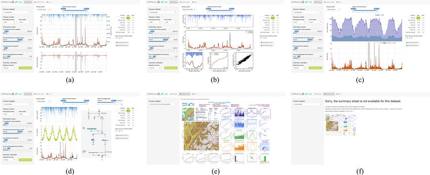
3940                                                 P. C. Astagneau et al.: Technical note: Hydrology modelling R packages

lected packages. The reader has to be aware that these might        of appropriate parameter estimation, i.e finding a consistent
have been adjusted from the original versions by the package        set of parameters. Among the practical outputs for a mod-
authors. We have, therefore, adopted a comparison method            eller, time series of actual evapotranspiration estimates can
that aims at representing the main principles behind the mod-       be useful for understanding the behaviour of the soil mois-
els – or differences in a perceptual model – but that still keeps   ture accounting functions. Retrieving time series of runoff
a certain degree of precision. This type of unified compari-        components (e.g. fast runoff and very quick runoff), which
son was, for example, employed in the framework for under-          are highlighted by Sect. 4.1, makes it possible to relate the
standing structural errors (FUSE; see Fig. 3 of Clark et al.,       model simulations with catchment regimes (e.g. high base-
2008) to compare the structures of four models or to present        flow well reproduced by the slow runoff exiting the ground-
the 40 models included in the MarRMOT toolbox (see Fig. 2           water store). Internal fluxes can inform a user on the inter-
of Knoben et al., 2019).                                            nal consistency of a simulation, for example, to identify the
   We selected an approach for this analysis that derives from      fraction of effective rainfall exiting the root zone store and
the work of de Boer-Euser et al. (2017, Fig. 3). This analy-        reaching the fast runoff routine compared to the fraction en-
sis aims at depicting the conceptual storages and fluxes at a       tering the groundwater store. Analysing time series of store
spatial unit scale. More details about the diagrams are given       levels can, for instance, enlighten the user on whether the
in Sect. 4.1 and Fig. 1. This analysis was reviewed by the          root zone store capacity has been correctly estimated, which
package authors to ensure consistency.                              would then help to analyse the simulation of soil moisture
                                                                    seasonality by the model for the studied catchment.
2.2.2   Spatial distribution                                           Any modeller would need to understand these specificities
                                                                    in order to select and apply a model. We summarise these
Users must be aware of the spatial discretisation that is avail-    characteristics (requirements, time step and numerical reso-
able. Furthermore, some packages offer the possibility to ap-       lution and outputs) in Sect. 4.3.
ply different types of catchment discretisations for the same
model. We, therefore, present the different cases for the se-       2.3     Framework for analysing package practicalities
lected packages after introducing a special case that is snow
modelling spatial distribution.                                     The different packages implement a set of functionalities to
                                                                    operate the models, which can be more or less in line with the
2.2.3   Requirements and outputs                                    hydrological workflow, i.e. from data preparation to analysis
                                                                    of the results. These functionalities aim at easing and some-
Since hydrological models do not always rely on the same            times constraining the use of the model. One would expect
assumptions, their requirements, i.e. data inputs and number        to use all the functionalities required to consistently apply a
of adjustable parameters, can differ. As data availability can      specific model and avoid any supplementary source of errors.
sometimes be a restraining factor, it is essential for users to     One of the specificities of R packages is the provided doc-
be informed about the model data requirements. The pack-            umentation. The related description and examples must be
ages also allow the operation of the models at different time       complete to ensure the appropriate application of the mod-
steps and imply different types of numerical resolutions of         els. The user is guided by basic examples and is made aware
model equations. The different equations of a hydrological          of potential errors that can occur. Following the analysis of
model can be solved using different techniques. The equa-           functionalities and documentation, we present an analysis of
tions are solved analytically (the exact solution is determined     R implementation that should foster more rigorous applica-
by integrating the equation for a given time step), explicitly      tions of the models. In an effort to contribute to more exten-
(the solution is approximated by its derivative at the begin-       sive documentation relating to the packages and their mod-
ning of the time step) or implicitly (the solution is approxi-      els, we provide R scripts enabling the use of each package on
mated by its derivative at the end of the time step). When the      simple examples. A short analysis of central processing unit
solution is analytical or explicit, the operator splitting tech-    (CPU) times is derived from the application of these scripts.
nique (OS) is commonly applied to solve the model equa-
tions. When OS is applied, the different processes, such as         2.3.1    Functionalities
evaporation, runoff and percolation are calculated sequen-
tially (Santos et al., 2018b). Numerical solution in hydrol-        What a package provides in terms of functionalities is a
ogy can be seen as part of the mathematical model structure         distinguishing feature when selecting a specific software or
rather than software implementation, as it changes the results      another programming language for hydrological modelling.
substantially (Clark and Kavetski, 2010; Kavetski and Clark,        Among the main features, we usually find the careful prepa-
2010).                                                              ration of input data to respect the right time references, ini-
   By making different outputs available, R packages allow          tialisation period or specific R objects. Enabling an automatic
modellers to better assess the suitability of applying a model      calibration procedure to find a set of parameters consistent
for a specific problem. It can also facilitate the evaluation       with the catchment of study can be an important step for

Hydrol. Earth Syst. Sci., 25, 3937–3973, 2021                                        https://doi.org/10.5194/hess-25-3937-2021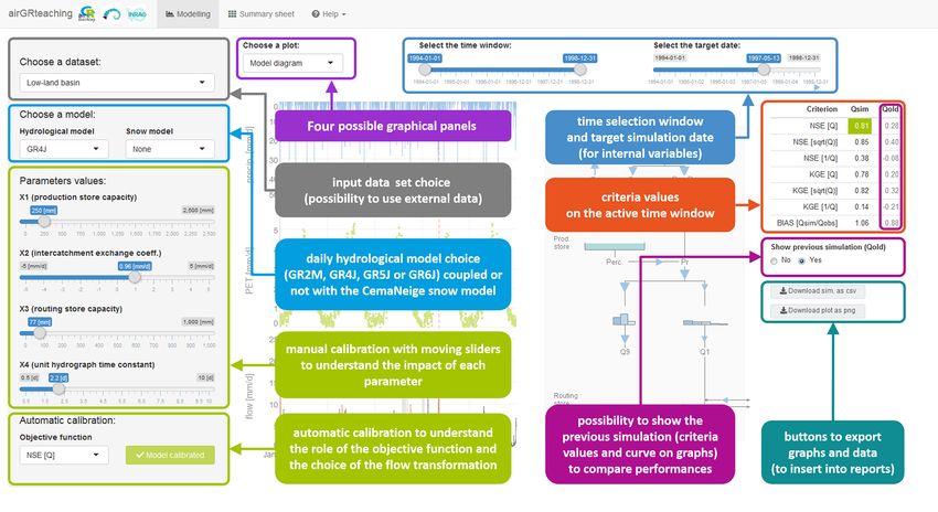
P. C. Astagneau et al.: Technical note: Hydrology modelling R packages                                                     3941

some models as well (though some packages have specifi-           required when creating a package but can be very useful for
cally avoided automatic calibration for the reasons discussed     a thorough understanding of the packages and models.
in Beven, 2012, 2016). Functions that allow the users to vi-
sualise and analyse the results are often appreciated. Sim-       2.3.3   User implementation
ple analyses can be the calculation of criteria assessing the
overall performance, for example. These criteria are regu-        Package practicalities can also be assessed through an anal-
larly calculated on time series of transformed data to empha-     ysis of the links between the main functions of a package.
sise specific error characteristics. Hydrograph plots are also    Such an examination could be useful to provide guidance re-
common for assessing hydrological models. Graphical user          garding package application. We try to put ourselves in the
interfaces can increase the package usability. As some mod-       shoes of users who have to apply the models of the different
els enable snow calculations, implementing an independent         packages and, therefore, need to understand which function
snow function is necessary to avoid using a snow function         they have to use, where to use it in the script and how to
on non-snowy catchments. One of the advantages of working         use it. In this regard, we propose a unified diagram of the
within the R framework is that the code can often be modified     connections between the main functions that we have been
by the user to access more variables or to calculate additional   able to run (see Fig. 4). We use the term user function, which
performance measures, etc., although some of the packages         means that users have to write their own R function integrat-
also include compiled components that might make this more        ing, among others, the legacies illustrated on the diagrams.
difficult.                                                        This analysis is intended for users familiar with R packages
   We present in this analysis whether the selected packages      and aims at guiding users in their application of the hydrolog-
integrate these basic functionalities to consistently apply the   ical modelling R packages. We, therefore, provide R scripts
models. Inspections of the packages were conducted based          enabling the application of each package on a simple hydrol-
on the different types of documents related to the packages       ogy example (Astagneau et al., 2020). The provided R scripts
and models. When judged necessary, the codes were anal-           show the basic R commands required to test one parameter
ysed to ensure accurate results.                                  set on two different catchments (see Sect. 2.3.4).

2.3.2   Documentation                                             2.3.4   R structures and CPU times

To handle the complexity associated with the different hy-        Package developers made several choices in terms of R im-
drological models and with the functionalities provided by        plementation that can affect package usability. For that rea-
the packages, the documentation is obviously essential for        son, we analyse the programming languages and external
any user. It is, therefore, important to assess whether looking   dependencies. We also perform a short analysis of package
at the overall documentation is sufficient to easily make use     CPU times.
of the package basics. In this regard, we compared the avail-         Some packages are entirely coded in R, which is an in-
able explanatory documents. This analysis is, by definition,      terpreted language, and some integrate models coded with a
subjective as it relies on our experience as users. However,      compiled programming language interfaced with R. The dif-
we think that it can still give insights into the meaningful      ferent programming languages interfaced with R were iden-
content of the documentation. Analysing the documentation         tified by extracting the package sources because they could
explanation by explanation would indeed be very compli-           not necessarily be identified by simply displaying the code
cated to present. There are the following two different types     from the R console. We considered a package as depen-
of documentation related to these packages: the R documen-        dent on external dependencies if one of its functions can-
tation that includes user manuals (functions explanations and     not be run without downloading another package. A pack-
mandatory for packages accepted by CRAN) and sometimes            age is not considered as being dependent on any other pack-
vignettes (“long-form guides that illustrate how to use pack-     age when the use of an external package is only suggested
ages”; Slater et al., 2019) and the external documentation that   in an example or in one of the related articles. Base pack-
comprise scientific journal articles and sometimes websites.      ages, such as stats, and recommended packages (https:
For each function of a package, the formal R user manual          //cran.r-project.org/src/contrib/3.6.0/Recommended, last ac-
includes mandatory fields (e.g. name, value, title, description   cess: 10 June 2021), such as lattice, are not taken into
and arguments) and optional fields (e.g. details, examples and    account in this assessment, as they are packages installed by
references; for more details see R Core Team, 2020b). We          default.
consider the following two types of scientific articles in this       From a user perspective, computation times can be mean-
analysis: articles written to present the packages and articles   ingful to determine whether a package is suitable for a spe-
using the packages and made by one of the package authors.        cific study. Short computation times are usually very well
Websites usually contain elements such as video tutorials, a      appreciated, especially when dealing with finer time steps or
list of publications mentioning the package, examples and         more complex spatial discretisations. Applying a model to a
user groups. Vignettes and external documentation are not         large database, generating an ensemble in operational (flood)

https://doi.org/10.5194/hess-25-3937-2021                                      Hydrol. Earth Syst. Sci., 25, 3937–3973, 2021
3942 P. C. Astagneau et al.: Technical note: Hydrology modelling R packages
forecasting or performing Monte Carlo runs for uncertainty – The RHMS package (Arabzadeh and Araghinejad, 2019)
analyses can also significantly increase computation times; implements several event-based hydrological models.
hence, some of the packages include some compiled code This package is not included in this work as we chose
to speed up the production runs of the model. We analysed to include only the continuous models.
the CPU time required for one model run, which was esti-
mated from 1000 runs with the microbenchmark pack- – The SWATmodel package (Fuka et al., 2014) im-
age (Mersmann, 2019). We ran the packages on a computer plements a complex watershed hydrological transport
with the following characteristics: random access memory model. This package does not provide any function for
(RAM) capacity – 8.00 GB; central processing unit (CPU) – data preparation or any explanatory document.
Intel i5-8250U 1.80 GHz; operating system (OS) – Windows
airGR
10 (64 bit), using the 3.6.0 (64 bit) R version. The mod-
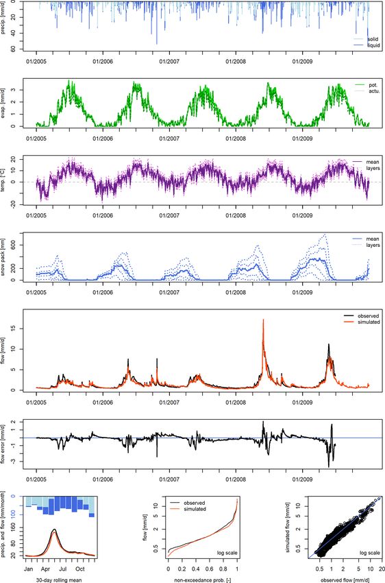
els were run at a daily time step on a catchment where The airGR package (Coron et al., 2020) implements the
high flows mostly result from precipitation events in win- models constituting the suite of Génie rural (GR) hydrolog-
ter, i.e. the Meuse River at Saint-Mihiel (2543 km2 ; from ical models (Coron et al., 2017) originating in the work of
1 January 1990 to 31 December 1999) and, for the packages Claude Michel, which started in the 1970s (Michel, 1983).
integrating a snow function, on a mountainous catchment These models are parsimonious conceptual rainfall–runoff
where high flows mostly result from snowmelt in spring, models that consider a catchment as a single entity (lumped).
i.e. the Ubaye River at Lauzet-Ubaye (943 km2 ; from 1 Jan- Several versions were developed over the years, from the
uary 1989 to 31 December 1998). The time series of precipi- well-known GR4J (Perrin et al., 2003) to the GR6J model
tation and temperature at a daily time step were extracted by (Pushpalatha et al., 2011), for improved low-flow simula-
Delaigue et al. (2020b) from the SAFRAN countrywide cli- tions. A snow accounting model called CemaNeige (Valéry
mate reanalysis of Météo-France (Vidal et al., 2010). The po- et al., 2014) can be combined with the daily and hourly GR
tential evapotranspiration (PET) time series were calculated models or can also be operated independently. airGR in-
using the Oudin et al. (2005) formula. The streamflow data cludes a function to calculate potential evapotranspiration
were retrieved from the “Banque Hydro” database (Leleu time series with the equation of Oudin et al. (2005). Vari-
et al., 2014). For the use of some packages, a digital elevation ous technical features associated with the hydrological work-
model (DEM) with a resolution of 25 m by 25 m was derived flow, from data preprocessing work to result analysis, are of-
from the BD ALTI DEM (IGN, 2013). Only one parameter fered. For the sake of brevity, only GR4J combined with Ce-
set is tested for each model. maNeige will be assessed in the following analyses. airGR
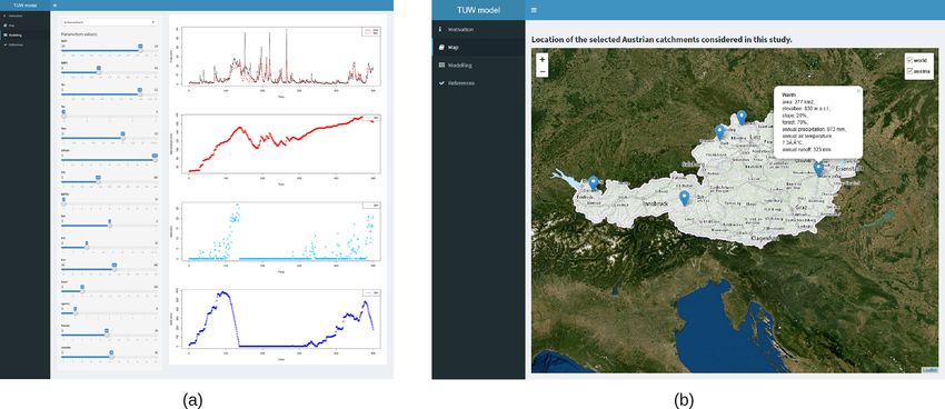
has a graphical user interface in the complementary pack-
3 An overview of the selected hydrological modelling R age airGRteaching (Delaigue et al., 2018, 2020a), which
packages will be analysed along with airGR.
The outcome of our selection is a list of eight packages that topmodel
will be carefully compared throughout the paper. Here we
The topography-based hydrological model (TOPMODEL;
give a first overview of these packages along with their re-
Beven and Kirby, 1979) has been employed for a variety
lated bucket-type hydrological models. The full list is pre-
of applications since its introduction (Beven et al., 2021).
sented in Table 1 with the main related documentation. Ta-
The TOPMODEL version included in topmodel (Buytaert,
ble 2 shows the snow models contained in the selected pack-
2018) follows the version developed by Beven et al. (1995)
ages.
that makes explicit assumptions about the nature of the near-
We chose to exclude the following packages, and we jus-
surface water table responses that lead to the possibility of
tify our choice in the following:
using a topographic wetness index (TWI) as an index of hy-
– The Ecohydmod package (Souza, 2017) implements drological similarity to calculate surface saturation and mois-
an ecohydrological model. ture deficits. Calculations are made for different increments
of the distribution of the index, making the model compu-
– The LWF-BROOK90 package (Schmidt-Walter et al.,
tationally fast to run. The pattern of the index can be de-
2020) implements a physically based land–surface hy-
rived from an analysis of a DEM and can be used to map
drological model.
the simulated response back into the space of the catchment.
– The fuse package (Vitolo et al., 2016b) proposes a topmodel allows simple calculations from a DEM and ba-
large number of model structure configurations. It was sic data series required in conceptual hydrological modelling.
considered that its main purpose was not to conduct a TOPMODEL allows for saturated contributing areas to be
basic hydrological study but more to understand errors predicted based on the spatial distribution of the topographic
arising from hydrological models. It is also in need of index. These assumptions mean that it is best suited to mod-
active maintenance. erately sloping hillslopes with relatively shallow water tables
Hydrol. Earth Syst. Sci., 25, 3937–3973, 2021 https://doi.org/10.5194/hess-25-3937-2021
P. C. Astagneau et al.: Technical note: Hydrology modelling R packages                                                                  3943

Table 1. A list of the selected packages with their related models. The models included in the following analyses are in bold. The models
included in hydromad that are presented in this table only correspond to the main soil moisture accounting functions (for more details, see
Andrews and Guillaume, 2018).

  Package               Version      Repository    Hydrological models         Main references for the models
  airGR                1.4.3.65      CRAN          GR1A; GR2M; GR4J;           Mouelhi (2003); Mouelhi et al. (2006); Perrin et al. (2003);
                                                   GR5J; GR6J;                 Le Moine (2008); Pushpalatha et al. (2011);
                                                   GR4H; GR5H                  Mathevet (2005); Ficchì et al. (2019)
  dynatopmodel             1.2.1     CRAN          Dynamic TOPMODEL            Beven and Freer (2001); Metcalfe et al. (2015)
  HBV.IANIGLA              0.1.1     CRAN          HBV                         Bergström (1976); Bergström and Lindström (2015)
  hydromad               0.9-26      GitHub        IHACRES-CMD;                Croke and Jakeman (2004);
                                                   IHACRES-CWI;                Jakeman and Hornberger (1993);
                                                   AWBM;                       Boughton (2004);
                                                   GR4J; Sacramento            Perrin et al. (2003); Burnash (1995)
  sacsmaR                  0.0.1     GitHub        Sacramento                  Burnash (1995)
  topmodel                 0.7.3     CRAN          TOPMODEL 1995               Beven and Kirby (1979); Beven et al. (1995)
  TUWmodel                1.1-1      CRAN          Modified HBV                Parajka et al. (2007)
  WALRUS                   1.10      GitHub        WALRUS                      Brauer et al. (2014a); Brauer et al. (2014b)

Table 2. A list of the snow models contained in the selected packages.

                           Package                Snow model                    Model reference
                           airGR                  CemaNeige                     Valéry et al. (2014)
                           dynatopmodel           None
                           HBV.IANIGLA            HBV                           Bergström and Lindström (2015)
                           hydromad               snow.sim                      Andrews and Guillaume (2018)
                           sacsmaR                SNOW-17                       Anderson (2006)
                           topmodel               None
                           TUWmodel               Modified HBV                  Parajka et al. (2007)
                           WALRUS                 Degree day method;            Seibert (1997)
                                                  shortwave radiation method    Kustas et al. (1994)

(see Quinn et al., 1991, for an application to a deeper sys-             lar aim of grouping parts of the catchment into computational
tem).                                                                    units for efficiency. The dynatopmodel package (Met-
                                                                         calfe et al., 2018) includes this model and offers the technical
dynatopmodel                                                             features to prepare the basic data required to run the dynamic
                                                                         TOPMODEL. For instance, a function to calculate a poten-
Driven by a desire to relax some of the assumptions of TOP-              tial evapotranspiration time series following the equation of
MODEL, the authors proposed a new version, i.e. the dy-                  Calder et al. (1983) is included.
namic TOPMODEL (Beven and Freer, 2001). In the orig-
inal version, simulations of subsurface flows depend on a                HBV.IANIGLA
quasi-steady-state assumption for the redistribution of mois-
ture at each time step (Beven, 1997). Dynamic TOPMODEL                   The HBV model (Bergström, 1976) has been improved over
relaxes this assumption to a non-steady kinematic wave so-               the years, one of its most employed version being the HBV-
lution for subsurface flows (between the similarity units) and           96 (Lindström et al., 1997). The HBV.IANIGLA package
allows other geographical information to be taken into ac-               (Toum, 2019) enables the application of each component (i.e.
count in the discretisation of the catchment – but with a simi-          snow, soil moisture and routing) of the HBV model indepen-

https://doi.org/10.5194/hess-25-3937-2021                                               Hydrol. Earth Syst. Sci., 25, 3937–3973, 2021
3944                                                P. C. Astagneau et al.: Technical note: Hydrology modelling R packages

dently. Other types of snow, soil moisture functions and rout-     research-departments/hydrology/hbv-1.90007, last access:
ing functions are also implemented, which are derived from         20 September 2020).
the HBV model (see Toum, 2019). This package also in-
cludes functions to calculate variables such as potential evap-    WALRUS
otranspiration, with the method of Calder et al. (1983), or
glacier discharge, with the equations of Jansson et al. (2003).    The WALRUS package (Brauer et al., 2017) contains the
                                                                   Wageningen lowland runoff simulator (WALRUS), a wa-
hydromad                                                           ter balance rainfall–runoff model that was specifically de-
                                                                   signed for catchments with shallow groundwater (Brauer
The hydrological model assessment and development pack-            et al., 2014a, b). This model assumes that each parameter
age hydromad (Andrews et al., 2011; Andrews and Guil-              has a physical meaning at the catchment scale (in a qualita-
laume, 2018) suggests the following two ways for treat-            tive sense). The WALRUS authors introduced the model as
ing rainfall–runoff modelling: either a single rainfall–runoff     an alternative to those mainly developed for sloping basins
model is considered, which can be a model such as Sacra-           (Brauer et al., 2014a) to better account for essential processes
mento (Burnash, 1995), or an effective rainfall framework is       in lowlands, such as capillarity rise and groundwater–surface
considered which distinguishes between a soil moisture ac-         water interactions. The package offers several functions in
counting (SMA) and a routing step, as in IHACRES (Jake-            line with the hydrological workflow. Snow accumulation and
man and Hornberger, 1993). A user has to choose the com-           melt can be calculated with one of the package functions
bination that best suits their requirements. hydromad in-          prior to the model simulations.
cludes 11 soil moisture accounting functions and six rout-
ing modules. A snow accounting function can be added
to the calculations when the IHACRES-CMD SMA is se-                4     A unified analysis of the hydrological models
lected. Several functions for data preprocessing, calibration            proposed in R packages
and post-treatment are made available by the package. In our
next analyses, for conciseness, we will only apply the Sacra-      4.1    Conceptual representation of storages and fluxes
mento, IHACRES and GR4J models.                                           through different model structures

sacsmaR                                                            The diagrams of Fig. 1 depict the conceptual storages and
                                                                   fluxes at a spatial unit scale (e.g. at the catchment or sub-
The sacsmaR package (Taner, 2019) implements the well-             catchment scale). For these diagrams, the root zone storage
known Sacramento soil moisture accounting model (SAC-              corresponds to the soil moisture accounting or production
SMA). In its original version, the SAC-SMA model was               function. Groundwater accounts for saturated soil zones and
set with lumped parameters. In the sacsmaR package, the            shallow aquifers involved in the catchment response. Fast
model can be run in a semi-distributed way. There is no pre-       runoff is similar to lateral flow or interflow. The term “very
processing function included in the package to deal with the       quick runoff” is used for processes with faster response times
spatial discretisation required to run the semi-distributed ver-   than “fast runoff” (de Boer-Euser et al., 2017). Bi-coloured
sion of SAC-SMA yet. A snow accounting module, SNOW-               rectangles are for two storages and/or fluxes modelled by the
17 (Anderson, 1976, 2006), can be run along with the SMA           same store or by the same function simultaneously. Please
and will be considered in our applications. A total of two         note that for the semi-distributed models, the schemes only
other functions are implemented in the package, i.e. a rout-       contain the storages and fluxes calculated on a single spa-
ing function based on Lohmann et al. (1996) and a function         tial unit. Details on the input data are given in Sect. 4.3. We
to calculate potential evapotranspiration time series based on     provide further explanations for each model hereafter.
the Hamon (1960) formulation.
                                                                   GR4J-CemaNeige
TUWmodel
                                                                   The combined GR4J and CemaNeige snow models are both
A modified version of the HBV rainfall–runoff model                included in airGR, meaning that total precipitation is first
(Bergström, 1976) is implemented in TUWmodel (Parajka              divided into solid and liquid precipitation by the snow func-
et al., 2007; Viglione and Parajka, 2020). HBV is com-             tion. Solid precipitation enters the snow accumulation store
posed of a snow routine, an SMA routine and a flow                 (light blue rectangle). Snowmelt (from the light blue rectan-
routing routine. The model can represent rainfall–runoff           gle) and liquid precipitation are added together to calculate
transformation in a lumped or semi-distributed way. In             interception (blue rectangle) considering PET. Then, either
comparison to other HBV versions, it does not imple-               a remaining PET component is used to calculate evapotran-
ment glacier melt modelling, refreezing of snow pack,              spiration withdrawn (blue and green arrows) from the pro-
separation of vegetation in different elevation zones or           duction store (green rectangle) or a part of the liquid pre-
lake impact on river flow (https://www.smhi.se/en/research/        cipitation remaining from the interception calculations either

Hydrol. Earth Syst. Sci., 25, 3937–3973, 2021                                       https://doi.org/10.5194/hess-25-3937-2021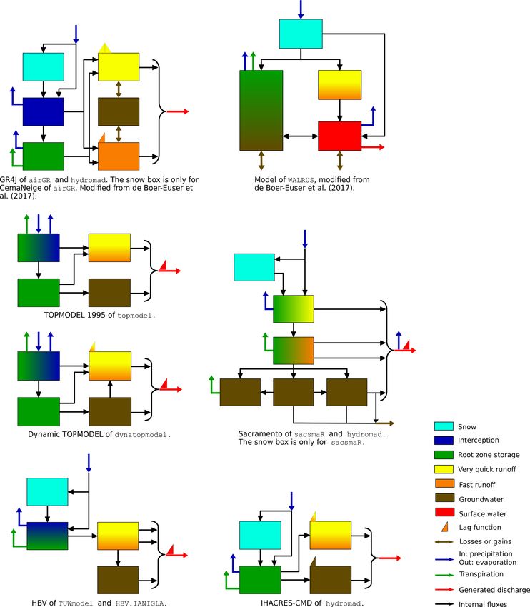
P. C. Astagneau et al.: Technical note: Hydrology modelling R packages                                                                  3945

Figure 1. Unified diagrams illustrating the depiction of conceptual storages and fluxes by the main models contained in the selected packages.

fills the production store or enters the very quick runoff and           GR4J model included in hydromad is almost identical to its
fast runoff unit hydrographs (UHs). A percolation compo-                 implementation in airGR. The difference is about the frac-
nent from the production store also joins the very quick (yel-           tion of water entering the fast runoff UH. This fraction was
low rectangle) and fast runoff (orange rectangle) UHs. The               empirically set to 0.9 in airGR, whereas this default value
output of the fast runoff UH fills a routing store. Water vol-           can be modified by the user in hydromad. The hydromad
umes can be added or withdrawn to/from the routing store                 package does not propose a snow function to be combined
or the very fast runoff component. This function accounts                with GR4J.
for groundwater contribution to runoff. The flow rate from
the routing store is then added to the very fast runoff compo-
nent to form the final discharge value at a particular time. The

https://doi.org/10.5194/hess-25-3937-2021                                               Hydrol. Earth Syst. Sci., 25, 3937–3973, 2021
3946                                                   P. C. Astagneau et al.: Technical note: Hydrology modelling R packages

WALRUS                                                                flow and will, thus, be routed along with the surface runoff.
                                                                      A constant celerity time delay function (or lag function) is
Precipitation is divided into solid or liquid water for the cal-      applied to route the sum of these two flows to the catchment
culation of snow accumulation and melt. Liquid precipitation          outlet.
and melt resulting from the snow function can either directly
join the surface water reservoir (red rectangle) or enter the         Dynamic TOPMODEL
wetness index calculation. The wetness index determines the
fraction of water infiltrating in the soil reservoir, which con-      The dynamic version of TOPMODEL (Beven and Freer,
tains both the vadose zone and saturated zone (green/brown            2001) is implemented in the dynatopmodel package and
reservoir) or joining the linear quick-flow reservoir (yellow         conceptual storages and fluxes of the dynamic TOPMODEL
to orange gradient rectangle) that supplies the surface wa-           are represented without taking the semi-distributed spatial-
ter reservoir. Evapotranspiration is retrieved from the surface       isation into account (i.e. on a single hydrological response
water reservoir and from the vadose zone both as a function           unit). Spatial characteristics of the package models will be
of PET and water contents. WALRUS integrates an explicit              dealt with in Sect. 4.2. The difference in terms of storages
representation of the dynamic water table in shallow ground-          and fluxes between the model in the topmodel package
water of lowland areas. The vadose zone concurrently inter-           and the model in the dynatopmodel package concerns the
acts with the groundwater through the dynamic water table             subsurface runoff and the water table. In the 1995 version of
in the same reservoir. The overall saturation of the soil reser-      TOPMODEL, the water table is represented as a succession
voir is governed by the dryness of the vadose zone, which             of quasi-steady states, whereas the dynamic TOPMODEL in-
determines the wetness index. The groundwater table depth             cludes a time-dependent kinematic routing (Beven and Freer,
is compared to the surface water level to determine either            2001; Metcalfe et al., 2015). The saturated zone (brown rect-
drainage towards the surface water or infiltration from the           angle) water level is predicted using implicit kinematic rout-
surface water. Discharge is a function of the surface water           ing between (and within) the spatial computational units.
level. Losses and gains can occur from/to the groundwater             When, within a unit, the local storage capacity is reached,
reservoir by seepage and from/to the surface water by ex-             any excess water is routed to downslope units (as a run-on)
traction or surface water supply.                                     or a connected river reach. Runoff components from the in-
                                                                      terception/root zone store, the unsaturated zone and the sat-
TOPMODEL 1995                                                         urated zone are added together (yellow to orange colour gra-
                                                                      dient rectangle) and then routed to the outlet by a constant
As briefly introduced in Sect. 3, two packages contain two            celerity time delay histogram.
different versions of TOPMODEL. Their singularities espe-
cially lie in the spatial distribution and calculations of subsur-    Sacramento
face contributions to streamflow. In terms of conceptual stor-
ages and fluxes, some small differences are highlighted by            In the Sacramento model of sacsmaR and hydromad,
our schematics. We first describe the water paths from inputs         snow calculations (precipitation separation and snow accu-
to outputs of TOPMODEL 1995 and then present the differ-              mulation and melt) prior to liquid water inputs of the hy-
ences brought by the dynamic TOPMODEL. Spatial consid-                drological model are only available within the sacsmaR
erations are dealt with in Sect. 4.2.                                 package. The Sacramento model represents the soil with two
   In the TOPMODEL 1995 version of topmodel, precipi-                 main layers, i.e. a thin upper layer and a thicker lower layer.
tation infiltrates first in the interception/root zone store (green   The upper layer contains two reservoirs (green to yellow and
to blue colour gradient), where the actual evapotranspiration         green to orange gradient rectangles), and the lower layer has
to be removed is calculated. When storage in the root zone is         three reservoirs (brown rectangles). Liquid water enters the
above a field capacity threshold, water is added to a drainage        first root zone store of the upper layer (green part of the
store (green rectangle) and recharge to the water table is cal-       green to yellow gradient rectangle), infiltrates through the
culated. At the end of each time step the configuration of            second root zone store (green part of the green to orange gra-
the saturated zone (brown rectangle) is updated according             dient rectangle) and then reaches the lower soil layer, where
to the topographic index distribution, as if the storage was          the three reservoirs are interconnected. Evaporation can oc-
in steady state with the drainage rate. On the saturated con-         cur from both the upper soil layer and the channel (blue ar-
tributing area, or where the unsaturated zone is filled from          row from the final red arrow). Plant transpiration can exit
above, an excess flow is transmitted to the overland routine          the upper soil layer and the lower soil layer. A very quick
(yellow to orange colour gradient). Consequently, the over-           runoff component originates from the first root zone store
land routine deals with storage excess coming from the satu-          (yellow part of the rectangle), which accounts for impervi-
rated zones, routes the runoff on the hillslopes and generates        ous area runoff. The second root zone store produces in-
a part of the flow that will then be routed by the channel rout-      terflow and another surface runoff component (both repre-
ing. The saturated zone drainage reaches the channel base-            sented by fast runoff, i.e. the orange part of the rectangle).

Hydrol. Earth Syst. Sci., 25, 3937–3973, 2021                                          https://doi.org/10.5194/hess-25-3937-2021
P. C. Astagneau et al.: Technical note: Hydrology modelling R packages 3947
The lower layer contributes to the baseflow channel compo- account (WALRUS, GR4J-CemaNeige, Sacramento, TUW-
nent and to a subsurface outflow lost by the model (brown model and IHACRES-CMD), the related calculations respect
arrow exiting the model). The baseflow channel component, similar steps where total rainfall (solid + liquid) is divided
the very quick runoff and the two fast runoff flows are added into solid precipitation, which supplies a snow cover stor-
together to form the final river discharge. A lag function can age, and liquid precipitation joining the hydrological model.
be applied on the final discharge. This function is based on These calculations follow a degree day approach, except for
Lohmann et al. (1996) when using the sacsmaR package. the snow model included in the sacsmaR package which
The hydromad package offers several routing functions that relies on a snow energy balance equation. WALRUS allows
can be applied as well. either a degree hour factor method or a shortwave radiation
factor method to be used. Both methods do not solve the en-
HBV ergy balance equation. In total three models, dynamic TOP-
MODEL, TOPMODEL 1995 and TUWmodel, take the inter-
In terms of conceptual storages and fluxes, the HBV model ception process into account with the root-zone-store-related
of TUWmodel and HBV.IANIGLA are similar. Precipita- calculations to reduce the number of parameters to be deter-
tion is first divided into snowfall and rainfall. Snowfall goes mined. Fast and very quick runoff are considered as being
to the snow routine (light blue rectangle) which calculates two distinct components for GR4J-CemaNeige, TUWmodel
snow accumulation and melt. The part of snow that melts and Sacramento. Apart from GR4J-CemaNeige, discharge
and rainfall become inputs of the root zone storage (blue sources are separated into a slow contribution from ground-
to green gradient rectangle). The soil moisture accounting water that can be identified as baseflow and a surface runoff
generates runoff and calculates actual evapotranspiration by input. These two components are added together to form the
taking potential evapotranspiration into account. The runoff final river discharge value, and sometimes, if not applied
generation routine consists of one upper reservoir and one separately before the addition (dynamic TOPMODEL and
lower reservoir with three outflows representing overland IHACRES-CMD), a lag function is employed on the over-
flow, interflow and baseflow. These runoff components are all resulting flow. WALRUS does not include such a function.
then routed by a triangular transfer function (red triangle; for Sacramento has a finer representation of soil layers compared
more details, please see Parajka et al., 2007). This function to the other models.
lags the overall flow volumes resulting from these three to
form the final discharge value. The differences between the 4.2 Which spatial distribution for which model?
HBV of HBV.IANIGLA and HBV of TUWmodel are as fol-
lows: HBV.IANIGLA offers the possibility to take glacier 4.2.1 The case of snow
discharge into account in the snow calculations, TUWmodel
distinguishes the temperature above which precipitation is As presented in the previous section, some packages enable
liquid from the temperature below which precipitation is the application of a snow function along with the hydro-
solid, and the time constant of the triangular function cor- logical models they include (airGR, HBV.IANIGLA,
responds to one parameter in HBV.IANIGLA, while it is de- hydromad only for IHACRES-CMD, sacsmaR,
rived from two different parameters in TUWmodel. TUWmodel and WALRUS). The influence of snow pro-
cesses on streamflow can vary with elevation, as snow
IHACRES-CMD
accumulation and melt mainly depend on air temperature
A simple degree day factor snow model (light blue) feeds, that usually decreases with elevation and precipitation that
with melt or liquid precipitation, into a catchment mois- usually increases with elevation. For that reason, a spatial
ture deficit model that represents soil moisture accounting discretisation within the catchment may be needed to better
(green). Evapotranspiration occurs from this store. The re- account for snow influence when modelling streamflow at
sulting effective rainfall is passed to a unit hydrograph, typi- the outlet of a catchment. Some packages propose a spatial
cally consisting of two flow paths (very quick/fast and slower discretisation to account for the influence of snow processes
groundwater) but with the potential for other configurations. on streamflow. A total of four configurations were found
These two runoff components are then added together to possible.
form the final discharge value. All these packages allow one to proceed with snow cal-
culations considering the catchment as a single unit. In
Synthesis that case, input data are aggregated at the catchment scale.
HBV.IANIGLA, hydromad and WALRUS do not offer any
This unified representation of the model structures in terms other possibility regarding the spatial distribution of snow
of conceptual storages and fluxes reveals certain trends in processes. The CemaNeige model of airGR is applied on
the different modelling choices. Although it is clear that different elevation zones of the catchment in order to take
each structure has its own specificities, the schematics high- into account the important heterogeneity of snow. The eleva-
light several modelling similarities. When snow is taken into tion bands have the same surface area (see Fig. 2). They are
https://doi.org/10.5194/hess-25-3937-2021 Hydrol. Earth Syst. Sci., 25, 3937–3973, 20213948 P. C. Astagneau et al.: Technical note: Hydrology modelling R packages
derived from the quantiles of the basin hypsometric curve HSUs (for more details, see Metcalfe et al., 2015, 2018). This
that must be provided to airGR. Precipitation and temper- also allows for connectivity between grids within the same
ature data are interpolated for each zone and become inputs HSU. Inputs can be spatially distributed, if needed, by asso-
of the CemaNeige model. There is one set of parameters for ciating each HSU with different rainfall and evapotranspira-
the whole basin. The spatial distribution of snow processes tion data. HSUs, thus, have their own reservoirs. When it is
by the TUWmodel and sacsmaR (SNOW-17 module) pack- required, a different parameter set can be assigned to every
ages follow another principle. The difference is that the ele- HSU.
vation zones can be set with different ranges and with dif- The HBV model of TUWmodel enables a very straight-
ferent surface areas (e.g. Fig. 2). Model parameters can be forward spatial configuration where the model is run inde-
differentiated across elevation zones. pendently on different zones (with different parameters and
inputs) which can be subbasins, elevation zones or any area
4.2.2 From lumped models to complex defined by the user. For example, a catchment can be divided
semi-distributions into three subbasins, with one subbasin divided into five ele-
vation zones. The relative contribution of each spatial entity
In the case of our selected models, the packages theoretically to the entire catchment is defined by the user with a weight-
allow one or more of the spatial discretisation configurations ing coefficient. The discharge outputs from each zone are
illustrated in Fig. 3. Table 3 summarises the possible config- then summed up using these coefficients. The Sacramento
urations for each model contained in the selected packages. model of sacsmaR can be applied in different ways. Dur-
When the models are applied with a lumped spatial config- ing a preprocessing step (not provided by the package func-
uration, inputs of precipitation and potential evapotranspira- tions), the catchment can be divided into sub-catchments that
tion are aggregated on the whole catchment. There is one set can also include hydrological response units. The sacsmaR
of parameters, which means that the model reservoirs rep- package then enables the assignment of a different set of pa-
resent the water content at the catchment scale. The model rameters to each HRU and different data inputs. The water
simulates a discharge output at the catchment outlet where is run upstream to downstream through a hydraulic routing
the hydrometric record station is located. function based on Lohmann et al. (1996).
TOPMODEL 1995 does not rely on the same calculations A large proportion of the packages that we have selected
as dynamic TOPMODEL, especially regarding the compu- contain models that can be run as lumped models, though
tational units. In this implementation of TOPMODEL 1995, some of them can rely on a more complex spatial distri-
inputs of precipitation and potential evapotranspiration are bution with very specific characteristics. The most complex
aggregated over the entire catchment (as a lumped model) level of the spatial distribution is enabled by the sacsmaR
although, in the original paper (Beven and Kirby, 1979), dif- package (HRUs + subbasins). Theoretically, it would be pos-
ferent inputs and TWI distributions were applied in differ- sible to run every lumped model on subbasins independently
ent sub-catchments. A single parameter set is defined at the and sum the outputs with weights, as permitted by one of the
catchment scale. Routines are provided for processing a dig- TUWmodel functions. We have noticed that there are thin
ital elevation model to calculate a topographic wetness in- boundaries between the different spatial configurations. One
dex for each grid cell (as a distributed model). The digital would hardly acknowledge the differences between a com-
elevation model should have a resolution of less than 30 m putational unit of TOPMODEL 1995 and HSUs of dynamic
for the results to be meaningful (Beven, 2012). Cells with TOPMODEL defined by the upslope area calculations. Nev-
similar values of the topographic index are then bundled to ertheless, these specificities can have a great influence on
create computational units. Each unit has specific reservoirs, the final result and, consequently, the interpretations deriving
while the saturation zone is represented as a global satura- from it. Please note that the high level of spatial discretisa-
tion value at the catchment scale. These units are intercon- tion enabled by some of the packages sometimes requires a
nected through the subsurface store updating based on the demanding preprocessing to be carried out outside of the cor-
TOPMODEL theory and produce runoff and baseflow val- responding package (e.g. sacsmaR; see Sect. 5 and Table 6).
ues to generate the final discharge time series (see Fig. 1). In addition, please note that the recently released version of
They can be seen as being a particular case of hydrological airGR (v. 1.6.10.4) allows for semi-distributed modelling at
response units (HRUs or hydrological similarity units, HSUs, the sub-catchment scale using a simple lag. As this version of
in Beven and Freer, 2001) resulting from explicit assump- airGR was released after the realisation of the present analy-
tions about the process response. Dynamic TOPMODEL en- sis, it is not included in Table 3.
ables the application of other types of HSUs that can be de-
pendent on very different conditions, such as soil properties
and land use but also the components of the topographic
index. Fluxes between HSUs are controlled by a flux dis-
tribution matrix based on the connectivity between the grid
squares of the base digital elevation map contributing to the
Hydrol. Earth Syst. Sci., 25, 3937–3973, 2021 https://doi.org/10.5194/hess-25-3937-2021You can also read