Climate model projections from the Scenario Model Intercomparison Project (ScenarioMIP) of CMIP6 - Earth System Dynamics
←
→
Page content transcription
If your browser does not render page correctly, please read the page content below
Earth Syst. Dynam., 12, 253–293, 2021
https://doi.org/10.5194/esd-12-253-2021
© Author(s) 2021. This work is distributed under
the Creative Commons Attribution 4.0 License.

            Climate model projections from the Scenario Model
             Intercomparison Project (ScenarioMIP) of CMIP6
                Claudia Tebaldi1 , Kevin Debeire2,3 , Veronika Eyring2,4 , Erich Fischer5 , John Fyfe6 ,
          Pierre Friedlingstein7,8 , Reto Knutti5 , Jason Lowe9,10 , Brian O’Neill11,a , Benjamin Sanderson12 ,
                  Detlef van Vuuren13 , Keywan Riahi14 , Malte Meinshausen15 , Zebedee Nicholls15 ,
             Katarzyna B. Tokarska5 , George Hurtt16 , Elmar Kriegler17 , Jean-Francois Lamarque18 ,
            Gerald Meehl18 , Richard Moss1 , Susanne E. Bauer19 , Olivier Boucher20 , Victor Brovkin21,b ,
         Young-Hwa Byun22 , Martin Dix23 , Silvio Gualdi24 , Huan Guo25 , Jasmin G. John25 , Slava Kharin6 ,
        YoungHo Kim26,c , Tsuyoshi Koshiro27 , Libin Ma28 , Dirk Olivié29 , Swapna Panickal30 , Fangli Qiao31 ,
           Xinyao Rong32 , Nan Rosenbloom18 , Martin Schupfner33 , Roland Séférian34 , Alistair Sellar9 ,
        Tido Semmler35 , Xiaoying Shi36 , Zhenya Song31 , Christian Steger37 , Ronald Stouffer38 , Neil Swart6 ,
        Kaoru Tachiiri39 , Qi Tang40 , Hiroaki Tatebe39 , Aurore Voldoire34 , Evgeny Volodin41 , Klaus Wyser42 ,
                           Xiaoge Xin43 , Shuting Yang44 , Yongqiang Yu45 , and Tilo Ziehn23
                1 Joint      Global Change Research Institute (JGCRI), Pacific Northwest National Laboratory,
                                                           College Park, MD, USA
                    2 Deutsches Zentrum für Luft- und Raumfahrt (DLR), Institut für Physik der Atmosphäre,

                                                         Oberpfaffenhofen, Germany
           3 Deutsches Zentrum für Luft- und Raumfahrt (DLR), Institut für Datenwissenschaften, Jena, Germany
                        4 Institute of Environmental Physics (IUP), University of Bremen, Bremen, Germany
                          5 ETH Zurich, Institute for Atmospheric and Climate Science, Zurich, Switzerland
              6 Canadian Centre for Climate Modelling and Analysis, Environment and Climate Change Canada,

                                                            Victoria, BC, Canada
                 7 College of Engineering, Mathematics and Physical Sciences, University of Exeter, Exeter, UK
                    8 LMD/IPSL, ENS, PSL Université, Ècole Polytechnique, Institut Polytechnique de Paris,

                                                  Sorbonne Université, CNRS, Paris, France
                                                   9 Met Office Hadley Center, Exeter, UK
      10 Priestley International Center for Climate, School of Earth and Environment, University of Leeds, Leeds, UK
                      11 Josef Korbel School of International Studies, University of Denver, Denver, CO, USA
            12 CNRS/Centre Européen de Recherche et de Formation Avancée en Calcul Scientifique (CERFACS),

                                                               Toulouse, France
                        13 PBL Netherlands Environmental Assessment Agency and Faculty of Geosciences,

                                                 Utrecht University, Utrecht, the Netherlands
                               14 International Institute for Applied Systems Analysis, Laxenburg, Austria
           15 Climate & Energy College, School of Earth Sciences, University of Melbourne, Melbourne, Australia
                    16 Department of Geographical Sciences, University of Maryland, College Park, MD, USA
                              17 Potsdam Institute for Climate Impact Research (PIK), Potsdam, Germany
        18 Climate and Global Dynamics Laboratory, National Center for Atmospheric Research, Boulder, CO, USA
                                    19 NASA Goddard Institute for Space Studies, New York, NY, USA
                               20 Institut Pierre-Simon Laplace, Sorbonne Université/CNRS, Paris, France
                                        21 Max Planck Institute for Meteorology, Hamburg, Germany
      22 National Institute of Meteorological Sciences/Korea Meteorological Administration, Seogwipo, South Korea
                                     23 CSIRO Oceans and Atmosphere, Aspendale, Victoria, Australia
                           24 Centro Euro-Mediterraneo sui Cambiamenti Climatici (CMCC), Bologna, Italy
                             25 NOAA/OAR/Geophysical Fluid Dynamics Laboratory, Princeton, NJ, USA

Published by Copernicus Publications on behalf of the European Geosciences Union.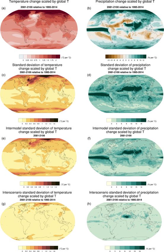
254                                                C. Tebaldi et al.: Climate model projections from ScenarioMIP of CMIP6

        26 Ocean   Circulation & Climate Change Research Center, Korea Institute of Ocean Science and Technology,
                                                            Busan, South Korea
                                         27 Meteorological Research Institute, Tsukuba, Japan
       28 Earth System Modeling Center, Nanjing University of Information Science and Technology, Jiangsu, China
                                         29 Norwegian Meteorological Institute, Oslo, Norway
                                        30 Indian Institute of Tropical Meteorology, Pune, India
               31 First Institute of Oceanography (FIO), Ministry of Natural Resources (MNR), Qingdao, China
         32 State Key Laboratory of Severe Weather, Chinese Academy of Meteorological Sciences, Beijing, China
                                        33 Deutsches Klimarechenzentrum, Hamburg, Germany
                            34 CNRM, Université de Toulouse, Météo-France, CNRS, Toulouse, France
           35 Alfred Wegener Institute, Helmholtz Centre for Polar and Marine Research, Bremerhaven, Germany
                                       36 Oak Ridge National Laboratory, Oak Ridge, TN, USA
                                             37 Deutscher Wetterdienst, Offenbach, Germany
                                                38 University of Arizona, Tucson, AZ, USA
                   39 Research Institute for Global Change (RIGC), Japan Agency for Marine-Earth Science

                                            and Technology (JAMSTEC), Yokohama, Japan
                                 40 Lawrence Livermore National Laboratory, Livermore, CA, USA
                                41 Institute of Numerical Mathematics, Moscow, Russian Federation
                            42 Swedish Meteorological and Hydrological Institute, Norrköping, Sweden
                         43 Beijing Climate Center, China Meteorological Administration, Beijing, China
                                      44 Danish Meteorological Institute, Copenhagen, Denmark
                   45 LASG, Institute of Atmospheric Physics, Chinese Academy of Sciences, Beijing, China
                                   a currently at: Joint Global Change Research Institute (JGCRI),

                                  Pacific Northwest National Laboratory, College Park, MD, USA
        b also at: Center for Earth System Research and Sustainability, University of Hamburg, Hamburg, Germany
                   c also at: Department of Oceanography, Pukyong National University, Busan, South Korea

                              Correspondence: Claudia Tebaldi (claudia.tebaldi@pnnl.gov)

                               Received: 28 August 2020 – Discussion started: 16 September 2020
                         Revised: 5 January 2021 – Accepted: 20 January 2021 – Published: 1 March 2021

      Abstract. The Scenario Model Intercomparison Project (ScenarioMIP) defines and coordinates the main set
      of future climate projections, based on concentration-driven simulations, within the Coupled Model Intercom-
      parison Project phase 6 (CMIP6). This paper presents a range of its outcomes by synthesizing results from the
      participating global coupled Earth system models. We limit our scope to the analysis of strictly geophysical out-
      comes: mainly global averages and spatial patterns of change for surface air temperature and precipitation. We
      also compare CMIP6 projections to CMIP5 results, especially for those scenarios that were designed to provide
      continuity across the CMIP phases, at the same time highlighting important differences in forcing composi-
      tion, as well as in results. The range of future temperature and precipitation changes by the end of the century
      (2081–2100) encompassing the Tier 1 experiments based on the Shared Socioeconomic Pathway (SSP) scenar-
      ios (SSP1-2.6, SSP2-4.5, SSP3-7.0 and SSP5-8.5) and SSP1-1.9 spans a larger range of outcomes compared
      to CMIP5, due to higher warming (by close to 1.5 ◦ C) reached at the upper end of the 5 %–95 % envelope of
      the highest scenario (SSP5-8.5). This is due to both the wider range of radiative forcing that the new scenarios
      cover and the higher climate sensitivities in some of the new models compared to their CMIP5 predecessors.
      Spatial patterns of change for temperature and precipitation averaged over models and scenarios have familiar
      features, and an analysis of their variations confirms model structural differences to be the dominant source of
      uncertainty. Models also differ with respect to the size and evolution of internal variability as measured by in-
      dividual models’ initial condition ensemble spreads, according to a set of initial condition ensemble simulations
      available under SSP3-7.0. These experiments suggest a tendency for internal variability to decrease along the
      course of the century in this scenario, a result that will benefit from further analysis over a larger set of models.
      Benefits of mitigation, all else being equal in terms of societal drivers, appear clearly when comparing scenarios
      developed under the same SSP but to which different degrees of mitigation have been applied. It is also found
      that a mild overshoot in temperature of a few decades around mid-century, as represented in SSP5-3.4OS, does
      not affect the end outcome of temperature and precipitation changes by 2100, which return to the same levels
      as those reached by the gradually increasing SSP4-3.4 (not erasing the possibility, however, that other aspects

Earth Syst. Dynam., 12, 253–293, 2021                                                 https://doi.org/10.5194/esd-12-253-2021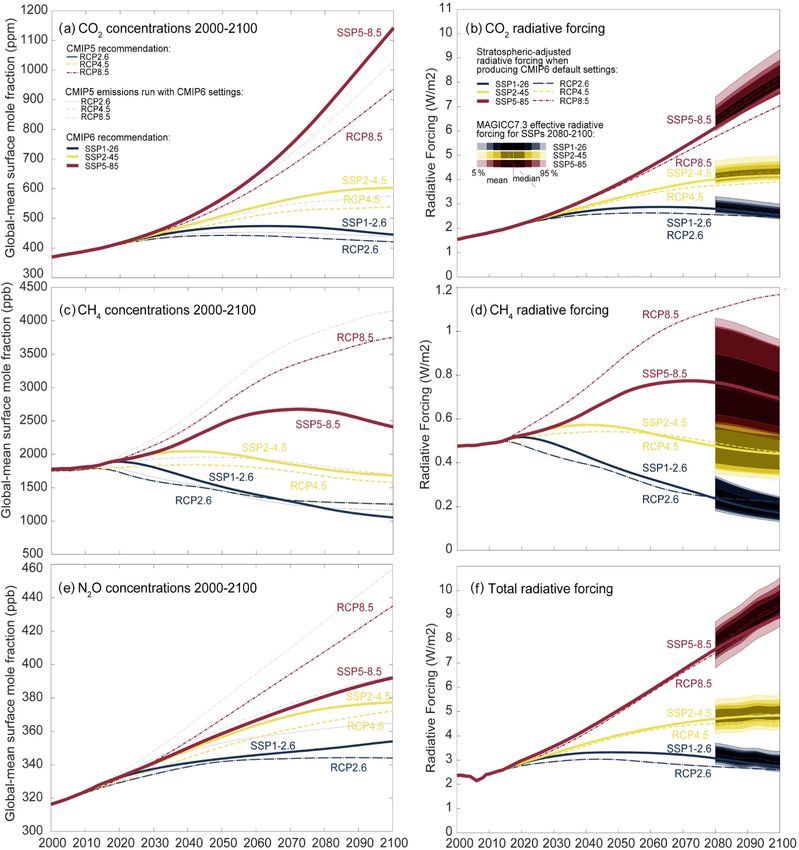
C. Tebaldi et al.: Climate model projections from ScenarioMIP of CMIP6                                                         255

       of the system may not be as easily reversible). Central estimates of the time at which the ensemble means of
       the different scenarios reach a given warming level might be biased by the inclusion of models that have shown
       faster warming in the historical period than the observed. Those estimates show all scenarios reaching 1.5 ◦ C
       of warming compared to the 1850–1900 baseline in the second half of the current decade, with the time span
       between slow and fast warming covering between 20 and 27 years from present. The warming level of 2 ◦ C of
       warming is reached as early as 2039 by the ensemble mean under SSP5-8.5 but as late as the mid-2060s under
       SSP1-2.6. The highest warming level considered (5 ◦ C) is reached by the ensemble mean only under SSP5-8.5
       and not until the mid-2090s.

1   Introduction                                                    given SSP, multiple levels of radiative forcings are achiev-
                                                                    able, given more or less stringent mitigation. Among this
                                                                    large set of scenarios, the ScenarioMIP design chose a sub-
Multi-model climate projections represent an essential
                                                                    set to be run by global climate and Earth system models
source of information for mitigation and adaptation deci-
                                                                    (ESMs) in concentration-driven mode. Some were chosen
sions. O’Neill et al. (2016) describe the origin, rationale and
                                                                    specifically to provide continuity with the RCPs: SSP1-2.6,
details of the experimental design for the Scenario Model In-
                                                                    SSP2-4.5, SSP4-6.0 and SSP5-8.5, where 2.6 to 8.5 stand
tercomparison Project (ScenarioMIP) for the Coupled Model
                                                                    for the stratospheric-adjusted radiative forcing in W m−2 by
Intercomparison Project phase 6 (CMIP6; Eyring et al.,
                                                                    the end of the 21st century as estimated by the IAMs. Ad-
2016). The experiments produce projections for a set of eight
                                                                    ditional trajectories were also chosen to fill in gaps in the
new 21st century scenarios based on the Shared Socioeco-
                                                                    previous scenario set for both baseline and mitigation sce-
nomic Pathways (SSPs) and developed by a number of inte-
                                                                    narios (SSP5-3.4; SSP3-7.0). Yet another was chosen to ad-
grated assessment models (IAMs). Extensions beyond 2100
                                                                    dress new policy objectives (SSP1-1.9, designed to meet the
based on idealized pathways of anthropogenic forcings are
                                                                    1.5 ◦ C target at the end of the century). The request of pri-
also included (formalized in their protocol by Meinshausen
                                                                    oritizing initial condition ensemble members for only one
et al., 2020), together with the request for a large initial con-
                                                                    of the scenarios (SSP3-7.0) was aimed at gathering sizable
dition ensemble under one of the 21st century scenarios. Two
                                                                    ensembles (10 members or more) from various modeling
of the scenarios are concentration overshoot (peak and de-
                                                                    centers. This was decided in recognition of the important
cline) trajectories, while the majority follow a traditional in-
                                                                    role of internal variability in contributing to future changes,
creasing or stabilizing trajectory.
                                                                    whose exploration is facilitated by initial condition ensem-
   The new scenarios are the result of an intense research
                                                                    bles (Deser et al., 2020; Santer et al., 2019). It was also rec-
phase that produced a new systematic scenario approach, the
                                                                    ognized that the spread in aerosol scenarios in the four RCPs
SSP-RCP (Representative Concentration Pathway) frame-
                                                                    used in CMIP5 was too narrow, as all assumed a large re-
work (van Vuuren et al., 2013), which relates the newer so-
                                                                    duction in atmospheric aerosol emissions (Moss et al. 2010,
cioeconomic scenarios to the RCPs first adopted in CMIP5
                                                                    Stouffer et al., 2017). The new SSP-based scenarios bet-
(Moss et al., 2010; Taylor et al., 2012). New qualitative nar-
                                                                    ter address this uncertainty by sampling a larger range of
ratives and future pathways of socioeconomic drivers (pop-
                                                                    aerosols pathways consistent with the corresponding green-
ulation, technology and gross domestic product; GDP) were
                                                                    house gas (GHG) emissions (Riahi et al., 2017). Scenario
developed according to two dimensions relevant to the cli-
                                                                    experiments were enabled by another community effort, in-
mate change problem, i.e., by positioning individual path-
                                                                    put4mip: based on the IAM emission trajectories, and after
ways as each representing a combination of low, medium
                                                                    harmonization of those to historical emission levels (Gidden
or high degrees of challenge to adaptation and to mitigation
                                                                    et al., 2019), a community effort took place to translate those
(O’Neill et al., 2013). Five such pathways (SSP1 through
                                                                    emission time series and amend them with additional input
SSP5) were developed. These were in turn used by IAMs
                                                                    fields for use by ESMs. These range from providing land-use
to produce scenarios of anthropogenic emissions and land
                                                                    patterns (https://doi.org/10.22033/ESGF/input4MIPs.1127),
use (Bauer et al., 2017; Riahi et al., 2017) consistent with
                                                                    gridded aerosol emission fields (Hoesly et al., 2018), strato-
the qualitative narratives and quantitative elements of each
                                                                    spheric aerosols (Thomason et al., 2018), solar irradiance
SSP. In addition to these baseline scenarios (i.e., scenarios
                                                                    time series (Mattes et al., 2017) and greenhouse gas concen-
that assume no explicit mitigation policies beyond those in
                                                                    trations (Meinshausen et al., 2020), as well as ozone fields
place at the time the scenarios were created, prior to the Paris
                                                                    (https://doi.org/10.22033/ESGF/input4MIPs.1115).
Agreement), a number of additional emissions and land-use
                                                                       Given the multi-model focus of CMIP and the overview
scenarios were produced that included mitigation policies
                                                                    purpose of this paper, the results reported here aim at giv-
(Kriegler et al., 2014) that achieved a range of radiative forc-
                                                                    ing a broad-scale representation of ensemble results (mean
ing targets for the end of the century. Thus, on the basis of a

https://doi.org/10.5194/esd-12-253-2021                                                Earth Syst. Dynam., 12, 253–293, 2021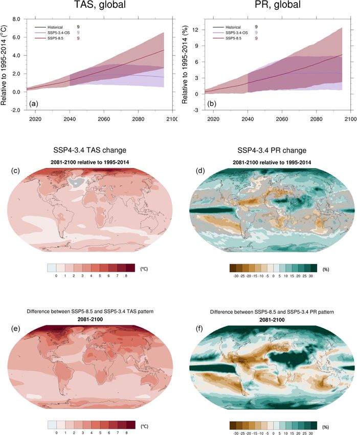
256                                                 C. Tebaldi et al.: Climate model projections from ScenarioMIP of CMIP6

and ranges or other measures of variability). The Scenar-          Only Tier 1, which can be satisfied by one realization per
ioMIP design responded to many complex objectives and             model, is required for participation in ScenarioMIP.
science questions, among which a high priority was the             Tier 2 completes the design by adding
need to lay the foundation for integrated research across
                                                                      – SSP1-1.9, informing the Paris Agreement target of
the geophysical, mitigation, impact, adaptation and vulner-
                                                                        1.5 ◦ C above pre-industrial;
ability research communities (O’Neill et al., 2020). The fo-
cus of this paper is to provide physical climate context for          – SSP4-3.4, a gap-filling mitigation scenario;
these more detailed analyses. Other model intercompari-
                                                                      – SSP4-6.0, an update of the CMIP5-era RCP6.0;
son projects (MIPs) within CMIP6 have prescribed experi-
ments that complement the ScenarioMIP design to address               – SSP5-3.4OS (overshoot), which tests the efficacy of an
questions about the effects of small radiative forcing dif-             accelerated uptake of mitigation measures after a de-
ferences, specific (and often local) forcings like those from           lay in curbing emissions until 2040: the scenario tracks
land use and short-lived climate forcers (SLCFs), the dif-              SSP5-8.5 until that date, then decreases to the same ra-
ferential effects of emission-driven vs. concentration-driven           diative forcing of SSP4-3.4 by 2100;
experiments testing the strength of the carbon cycle (Arora
et al., 2020) and the effectiveness of emergent constraints           – three extensions to 2300, two of them continuing on
in reshaping the uncertainty ranges of the new multi-model              from SSP1-2.6 and SSP5-8.5 and one extending the
ensemble (Nijsse et al., 2020; Tokarska et al., 2020). They             SSP5-3.4 overshoot pathway towards the lower radia-
are the Land Use MIP (LUMIP; Lawrence et al., 2016), the                tive forcing level of 2.6 W m−2 , to inform the analysis
Aerosol Chemistry MIP (AerChemMIP; Collins et al., 2017),               of long-memory processes, like ice-sheet melting and
the Coupled Climate-Carbon Cycle MIP (C4MIP; Jones et                   corresponding sea level rise;
al., 2016), the Geoengineering MIP (GeoMIP; Kravitz et                – nine additional initial condition ensemble members un-
al., 2015) and the Carbon Dioxide Removal MIP (CDRMIP;                  der SSP3-7.0 to explore internal variability and signal-
Keller et al., 2018).                                                   to-noise characteristics of the different participating
   In this study, we focus the analysis on the future evolu-            models.
tion of average temperatures and precipitation. We address
questions regarding the strength of the signal under the dif-     Here we note that although the labels identify the specific
ferent CMIP6 scenarios and compare to similar CMIP5 sce-          SSP used in the development of the scenario, the climate out-
narios: the identification of the time of separation between      comes are still intended to be combined with multiple differ-
the temperature trajectories under the different scenarios and    ent SSPs in integrated studies. A list of the participating mod-
the time at which they cross global warming thresholds. We        els, with references for documentation and data, is shown in
also analyze spatial patterns of change addressing questions      Table A1. Table A2 lists the CMIP5 models used in the com-
of robustness between the CMIP5 and CMIP6 multi-model             parisons.
ensembles and within the CMIP6 ensemble among models
and scenarios.                                                    3     Results

                                                                  For the results shown in this section, we extracted monthly
2   ScenarioMIP experiments and participating                     mean near-surface air temperature (TAS) and precipitation
    models                                                        (PR) from the models listed in Tables A1 and A2 (for CMIP5
                                                                  scenarios). These were averaged globally or separately over
As described in detail in O’Neill et al. (2016) and summa-        land and oceans for time series analysis (no correction for
rized in the matrix display in Fig. A1, the ScenarioMIP de-       drift was performed) and regridded to a common 1◦ grid by
sign consists of the following concentration-driven scenario      linear interpolation for pattern analysis. All figures of this
experiments, subdivided into two tiers to guide prioritization    paper are produced with the Earth System Model Evaluation
of computing resources. Tier 1 consists of four 21st cen-         Tool (ESMValTool) version 2.0 (v2.0) (Righi et al., 2020;
tury scenarios. Three of them provide continuity with CMIP5       Eyring et al., 2020; Lauer et al., 2020), a tool specifically de-
RCPs by targeting a similar level of aggregated radiative         signed to improve and facilitate the complex evaluation and
forcing (but we highlight important differences in the com-       analysis of CMIP models and ensembles.
ing discussion): SSP1-2.6, SSP2-4.5 and SSP5-8.5. An addi-
tional scenario, SSP3-7.0, fills a gap in the medium to high      3.1     Global temperature and precipitation projections for
end of the range of future forcing pathways with a new base-              Tier 1 and the SSP1-1.9 scenarios
line scenario, assuming no additional mitigation beyond what
                                                                  3.1.1    Time series
is currently in force. The same scenario also prescribes larger
SLCFs concentrations and land-use changes compared to the         Figure 1 shows time series of global mean surface air temper-
other trajectories.                                               ature (GSAT) and global precipitation changes (see Fig. A2

Earth Syst. Dynam., 12, 253–293, 2021                                                https://doi.org/10.5194/esd-12-253-2021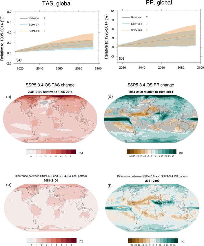
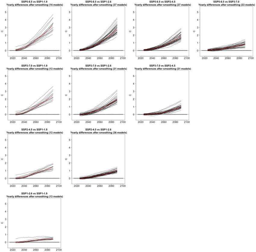
C. Tebaldi et al.: Climate model projections from ScenarioMIP of CMIP6                                                           257

for time series of the same variables disaggregated into land-     (between 33 and 39 for Tier 1 experiments). Only the number
only and ocean-only area averages; also see Tables A3 and          of models contributing to the lowest scenario (SSP1-1.9) is
A4 for changes under the different scenarios around mid-           significantly lower, i.e., 13 at the time of writing, but the anal-
century and the end of the century). The historical baseline       ysis of ensemble behavior of Sect. 3.2.1 below suggests that
is taken as 1995–2014 (2014 being the last year of CMIP6           for global temperature and precipitation averages 10 ensem-
historical simulations). The five scenarios presented in these     ble members provide a representative sample of the internal
plots consist of the Tier 1 experiments (SSP1-2.6, SSP2-4.5,       climate variability. The same qualitative behavior appears for
SSP3-7.0 and SSP5-8.5) and the additional scenario designed        land-only and ocean-only averages (Fig. A2 and Table A3),
to limit warming to 1.5 ◦ C above 1850–1900 (a period often        with the faster warming over land than ocean reaching on av-
used as a proxy for pre-industrial conditions), SSP1-1.9. We       erage up to 5.46 ◦ C under SSP5-8.5 (compared to the global
smooth each trajectory by an 11-year running mean to focus         average reaching 3.99 ◦ C) and some models reaching a much
on climate-scale variability.                                      larger value under this scenario of 7.57 ◦ C. For the lower sce-
   In the plots, the thick line traces the ensemble average        narios, limiting warming in 2100 to 0.69 and 1.23 ◦ C globally
(see legend and Table A1 for the number of models included         translates to an average warming on land of 0.96 and 1.61 ◦ C
in each scenario calculation) and the shaded envelopes rep-        for SSP1-1.9 and SSP1-2.6, respectively (see Table A3 for
resent the 5 %–95 % ranges, which are obtained assuming            all projections and their ranges referenced to the historical
a normal distribution as 1.64σ , where σ is the intermodel         baseline).
standard deviation of the smoothed trajectories, computed             In order to characterize when pairs of scenarios diverge,
for each year. Only one ensemble member (in the majority           we define separation as the first occurrence of a positive dif-
of cases r1i1p1f1) is used even when more runs are avail-          ference between two time series, one under the higher and
able for some of the models. By the end of the century (i.e.,      one under the lower forcing scenarios, which is then main-
as the mean of the period 2081–2100), the range of warm-           tained for the remainder of the century. This is similar to
ing spanned by the multi-model ensemble means under all            Tebaldi and Friedlingstein (2013, TF13 in the following),
scenarios is between 0.69 and 3.99 ◦ C relative to 1995–2014       who used the first occurrence of a significant trend in the
(0.84 ◦ C greater when using the 1850–1900 baseline). Con-         year-by-year differences, then justified by the RCPs under
sidering the multi-model ensemble means as the best esti-          consideration, among which only the lowest (RCP2.6) flat-
mates of the forced response under each scenario, the range        tened out over the century. In that case, the remainder of the
spanned by them can be interpreted as an estimate of sce-          RCPs considered followed an increasing trajectory, with dif-
nario uncertainty. When considering the shaded envelopes           ferential rates of increase, therefore justifying the expecta-
around the ensemble mean trajectories, about 0.6 at the lower      tion that year-by-year differences would eventually show a
end and 1.6 ◦ C at the upper end are added to this range.          significant and persisting trend. Among the new scenarios,
This range can be seen as reflecting the compound effects          at least two are expected to follow a flat trajectory, or even
of model-response uncertainty and some measure of internal         a slight peak and decline (SSP1-1.9 and SSP1-2.6), render-
variability in the individual model trajectories, but the latter   ing the expectation of a trend in their differences untenable.
is likely underestimated, given that we are using only one run     We therefore adopt a slightly different definition here, and
per model. The use of initial condition ensembles for each of      we also note that this definition would need to be modified
the models would better characterize their respective internal     if overshoot scenarios – crossing their reference as they de-
variability (Lehner et al., 2020). Using the 5 %–95 % confi-       crease – were the main focus of this analysis. Also, this is
dence intervals as ranges, we find that by the end of the 21st     not the only way to define separating scenarios, and other
century (2081–2100 average, always compared to the 1995–           studies have applied different, but still fairly similar, defini-
2014 average) global mean temperatures are projected to in-        tions, e.g., recently, Marotzke (2019). We use time series of
crease between 2.40 and 5.57 ◦ C for SSP5-8.5, between 1.95        GSAT after applying a 21-year running mean, as we are con-
and 4.38 ◦ C under SSP3-7.0, and between 1.27 and 3.00 ◦ C         cerned with differences in climate rather than in individual
for SSP2-4.5. Global temperatures stabilize or even some-          years, whose temperatures are affected by large variability
what decline in the second half of the century in SSP1-1.9         (this is the part of the definition that takes the place of the
and SSP1-2.6, which span a range from 0.13 to 1.25 ◦ C and         consideration of long-term trends in TF13). We also need to
0.40 to 2.05 ◦ C, respectively, whereas they continue to in-       choose a threshold at which we deem the difference “posi-
crease to the end of the century in all other SSPs. The ensem-     tive” and somewhat discernible (this takes the place of ask-
ble spread appears to consistently increase with the higher        ing for a significant trend in TF13). To do so, we use the re-
forcing and over time. This suggests that the model response       sults in Tebaldi et al. (2015), where the regional sensitivities
uncertainty increases for stronger responses, an expected re-      of temperature and precipitation to changes in global aver-
sult as climate sensitivity – which significantly differs among    age temperature were quantified. According to that analysis,
the models – more strongly influences the model response in        a 0.1 ◦ C difference in 20-year means of GSAT was the low-
higher scenarios and later periods (Lehner et al., 2020). This     est value at which a multi-model ensemble consistently had
result appears robust, given the number of models included         a positive fraction of the grid cells experiencing significant

https://doi.org/10.5194/esd-12-253-2021                                                Earth Syst. Dynam., 12, 253–293, 2021
258                                                     C. Tebaldi et al.: Climate model projections from ScenarioMIP of CMIP6

Figure 1. (a) Global average temperature time series (11-year running averages) of changes from current baseline (1995–2014, left axis)
and pre-industrial baseline (1850–1900, right axis, obtained by adding a 0.84 ◦ C offset) for SSP1-1.9, SSP1-2.6, SSP2-4.5, SSP3-7.0 and
SSP5-8.5. (b) Global average precipitation time series (11-year running averages) of percent changes from current baseline (1995–2014)
for SSP1-1.9, SSP1-2.6, SSP2-4.5, SSP3-7.0 and SSP5-8.5. Thick lines are ensemble means (number of models shown in the legends).
The shading represents the ±1.64σ interval, where σ is the standard deviation of the smoothed trajectories computed year by year (thus
approximating the 5 %–95 % confidence interval around the mean of a normal distribution). Note that the uncertainty bands are computed
for the anomalies with respect to the historical baseline (1995–2014). Thus, the right axis of the global temperature plot, showing anomalies
with respect to pre-industrial values, applies to the ensemble means, not to the uncertainty bands, which would be narrowest over the period
1850–1900 if we were to calculate uncertainties on the basis of the models’ output over that period, rather than by simply adding an offset
uniformly. See Fig. A2 for land-only and ocean-only averages and Tables A3 and A4 for the values of changes at mid- and late century.

warming. In Table A5, we report the precise years when the               ration of SSP3-7.0 from SSP5-8.5 (Fig. A3, black lines, and
ensemble means of the smoothed GSAT time series under the                values in parentheses in Table A5).
various scenario pairs separate according to this definition                 Ensemble mean precipitation change by 2081–2100 (as
and, in parentheses, when the last of all individual models’             a percentage of the 1995–2014 baseline) is between 2.0 %
pairs of trajectories separate, but of course those precise es-          and 3.0 % for the lowest scenarios (SSP1-1.9 and SSP1-2.6),
timates would change if our choices of the moving window                 4.2 % and 4.9 % for SSP2-4.5 and SSP3-7.0, and 7.3 % for
and the threshold had been different. The ensemble average               SSP5-8.5. As expected, the larger variability of precipitation
trajectory of GSAT under SSP5-8.5 separates from the lower               changes (relative to temperature changes), both from internal
scenarios’ ensemble average trajectories between 2027 and                sources and model response uncertainty, is such that only the
2034, with the longer time as expected applying to the sepa-             highest scenario ensemble mean trajectory separates from the
ration from SSP3-7.0. SSP3-7.0 separates from the two sce-               lower ones appreciably before 2050, while the lowest sce-
narios at the lower end of the range between 2031 and 2037,              nario separates from the rest around mid-century. The en-
and 10 years later from SSP2-4.5. The ensemble average tra-              semble means of the three scenarios in between overlap un-
jectory of global temperature under SSP2-4.5 separates from              til close to 2070. The multi-model spread and internal vari-
those under the two lower scenarios, SSP1-1.9 and SSP1-2.6,              ability confound a large fraction of the individual scenarios’
by 2034 and 2039, respectively, while the ensemble average               trajectories until the end of the century (Fig. 1b). Both the
GSAT trajectories under the two lower scenarios, SSP1-1.9                magnitude of the changes and their variability are larger for
and SSP1-2.6, separate from one another in 2042 (in Fig. A3,             precipitation averages over land than over oceans (Fig. A2;
the differences between ensemble averages for each pair of               see also Table A4 for a complete list of mid- and late-century
scenarios appear as red lines). When considering individual              changes).
models’ trajectories under the different scenarios and defin-
ing the time of separation when the last of all individual pair
                                                                         3.1.2   Normalized patterns
of trajectories separates, model structural differences and a
larger effect of internal variability cause a significant delay          In Fig. A4, we show ensemble average patterns of change by
compared to the ensemble mean separation. Depending on                   the end of the century under the five scenarios for both vari-
the pair of scenarios considered, the length of the delay nec-           ables. In this section, we focus our discussion on the gen-
essary for the last of the models to show separation varies sig-         eral features emerging from the average normalized patterns.
nificantly: as few as 6 years for the full separation of SSP1-           Normalized patterns are computed as the end-of-century
2.6 from SSP5-8.5 and as many as 19 years for the full sepa-             (percent) change compared to the historical baseline, di-
                                                                         vided by the corresponding change in global mean tempera-

Earth Syst. Dynam., 12, 253–293, 2021                                                        https://doi.org/10.5194/esd-12-253-2021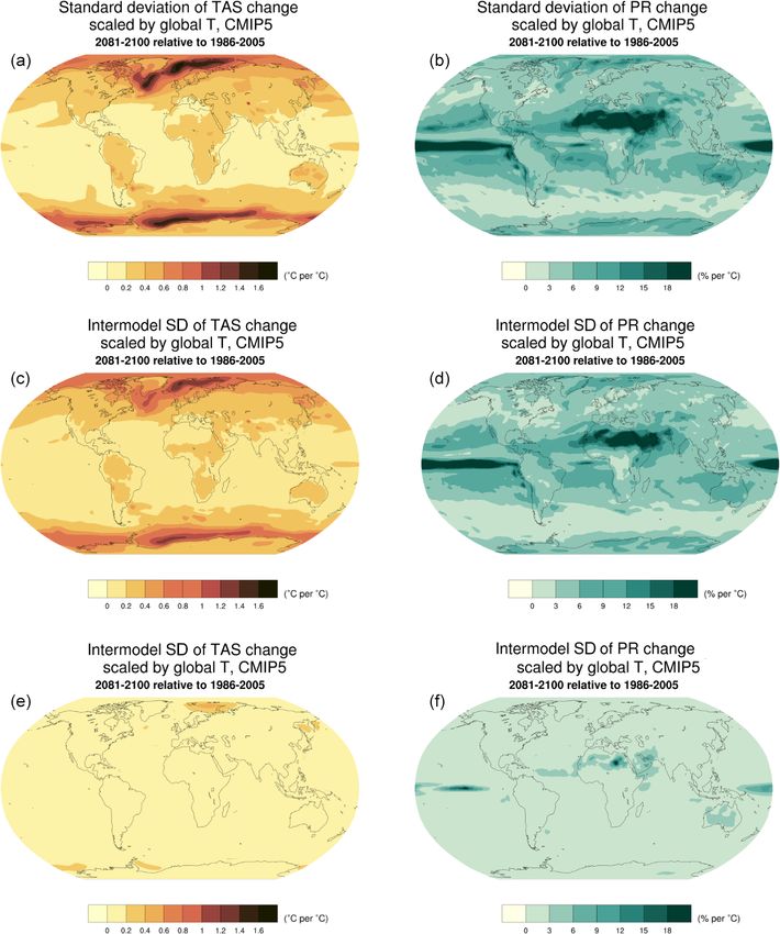
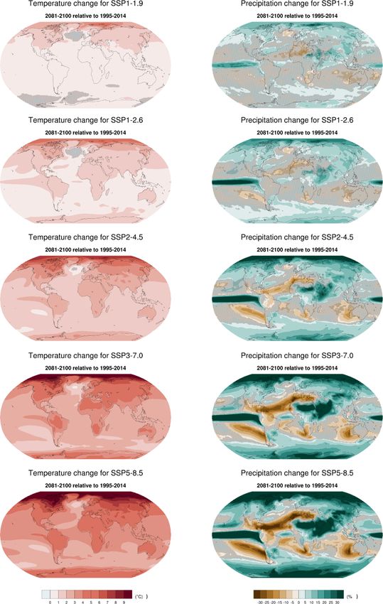
C. Tebaldi et al.: Climate model projections from ScenarioMIP of CMIP6                                                          259

ture. This computation is first performed for each individual       eas where models disagree, and scenarios, in lesser measure,
model or scenario, at each grid point, after regridding tem-        can be at odds due to their different timing of persistent ice
perature and precipitation output to a common 1◦ × 1◦ grid.         melt. The variability and therefore uncertainty of the precip-
The individual normalized patterns are then averaged across         itation pattern mirrors the signal of change at low latitudes in
models and the five scenarios. As we will show, the total vari-     the Pacific and over Africa and Asia. The comparison of pat-
ations among the population of normalized patterns that form        terns in the third and fourth rows of the figure elucidates the
this grand average are mainly driven by intermodel variabil-        role of intermodel variability rather than scenario variability
ity rather than interscenario differences. Thus, we choose to       for both temperature and precipitation normalized changes,
synthesize patterns of change across all scenarios by present-      with scenario uncertainty only contributing to a small area of
ing regional changes per degree of global warming. More in-         sea ice variability in the Arctic for temperature change and a
depth analyses, also exploiting complementary experiments           subregion of the Sahara for precipitation change (where the
from LUMIP and AerChemMIP, may provide a more refined               denominator of the percentage values is small and therefore
view of the interscenario differences possibly arising from         prone to cause instabilities in the values computed). Given
different regional forcings.                                        the radically different sample sizes used to compute the aver-
   Figure 2 (top row) shows the spatial characteristics             ages from which scenario-driven standard deviations are de-
of warming and of wetting and drying. For temperature               rived compared to model-driven ones (more than 30 for the
changes, the left panel confirms the well-established gradient      former and only five for the latter), we can also infer that in-
of warming decreasing from northern high latitudes (with the        ternal variability is a likely contributor to model-driven stan-
Arctic regions warming at twice the pace of the global aver-        dard deviation, while it is mostly eliminated before the com-
age) to the Southern Hemisphere and the enhanced warming            putation of the scenario-driven standard deviation.
in the interior of the continents compared to ocean regions            The robustness of these multi-model average patterns and
(which consistently warm slower than the global average).           the sources of their variability can be assessed by considering
This differential is particularly pronounced in the Northern        the same type of graphics computed from the four RCPs from
Hemisphere (and would be muted if the normalized pattern            the CMIP5 model ensemble.
was computed at equilibrium). The familiar cooling spot in             Figures 3 (top row) and A5, using the same color scales,
the northern Atlantic appears as well – the only region with        are easily compared to Fig. 2 and confirm the striking consis-
a negative sign of change. Studies have suggested that the          tency of the geographical features of the normalized patterns,
cooling signal is an effect of the slowing of the Atlantic          the size and spatial features of their variability, together with
Meridional Overturning Circulation, which creates a signal          the components of the latter (i.e., model vs. scenario variabil-
of slower northward surface-heat transport, resulting in an         ity).
apparent local cooling (Caesar et al., 2018; Keil et al., 2020).       We deem a rigorous quantification of the differences be-
   For precipitation, the strongest positive changes are in the     tween patterns beyond the scope of this paper and focus
equatorial Pacific and the highest latitudes of both hemi-          on a qualitative assessment of the similarities that surface
spheres, especially the Arctic region. The large changes in         by showing in the bottom row in Fig. 3 the difference be-
subtropical Africa and Asia are due more to the small pre-          tween CMIP6 and CMIP5 normalized patterns, confirming
cipitation amounts of the climatological averages in these re-      the small magnitude of the discrepancies in TAS over all re-
gions (at the denominator of these percent changes) than to a       gions, except for the Arctic, known to be affected by large
truly substantial increase in precipitation (see also below for     variations among models, scenarios (with a possible role of
variability considerations). A strong drying signal continues       the lowest scenario in CMIP6, SSP1-1.9, whose land–sea ra-
to be projected for the Mediterranean together with central         tio has likely no equivalent among the CMIP5 scenarios, but
America, the Amazon region, southern Africa and western             further, more rigorous investigation is needed to confirm this)
Australia.                                                          and internal noise (likely playing a minor role given the num-
   Similar to Tebaldi and Arblaster (2014), we give a measure       ber of models and scenarios contributing to these averages).
of robustness of these patterns by computing the standard de-       Similarly, for percent precipitation, the regions that stand out
viation at each grid point across individual model or scenario      where the largest differences are found are the tropics, known
patterns (Fig. 2, rows 2–4). We further distinguish the relative    to be affected by large variability and uncertainties. In this
contribution of scenario and model variability by computing         case, the possible role of aerosol forcing (Yip et al., 2011)
standard deviations after averaging across models separately        warrants further investigation, especially as we consider that
for each individual scenario and across scenarios for each          SSP3-7.0 forcing composition and trajectory are quite dif-
individual model, respectively. Figure 2, second row, high-         ferent from those of previous scenarios. As mentioned, the
lights in darker colors regions where the standard deviation is     use of these experiments in conjunction with their variants
higher and patterns are less robust. For temperature patterns,      by LUMIP and AerChemMIP could further attribute some of
as has been found in earlier studies of pattern scaling (starting   these scenario-dependent features to differences in regional
from Santer et al., 1990, and in more recent work, like Herger      forcing like land use or aerosols. Also, a subset of CMIP6
et al., 2015), the edges of sea ice retreat at both poles are ar-   models are running the CMIP5 RCPs, and results from those

https://doi.org/10.5194/esd-12-253-2021                                                 Earth Syst. Dynam., 12, 253–293, 2021
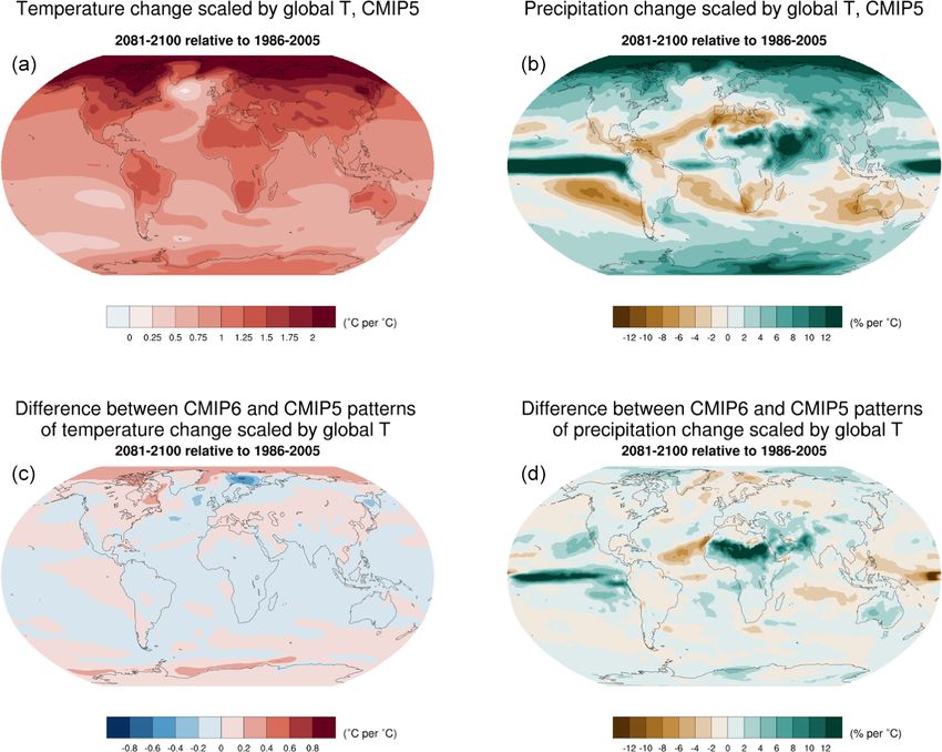
260                                                      C. Tebaldi et al.: Climate model projections from ScenarioMIP of CMIP6

Figure 2. (a, b) Patterns of temperature (a) and percent precipitation change (b) normalized by global average temperature change (averaged
across CMIP6 models and all Tier 1 plus SSP1-1.9 scenarios). (c, d) Standard deviation of normalized patterns for individual CMIP6
models and scenarios. The individual patterns are the elements from which the averages shown in the top row are computed. (e, f) Standard
deviation of normalized patterns, after averaging across scenarios, highlighting the role of intermodel variability. (g, h) Standard deviation
of normalized patterns after averaging across models, highlighting the role of interscenario variability.

Earth Syst. Dynam., 12, 253–293, 2021                                                         https://doi.org/10.5194/esd-12-253-2021
C. Tebaldi et al.: Climate model projections from ScenarioMIP of CMIP6                                                            261

Figure 3. Patterns of temperature (a) and percent precipitation change (b) normalized by global average temperature change (averaged
across models and scenarios) from CMIP5 models and scenarios, for comparison with Fig. 2 (top row). Panels (c) and (d) show differences
between CMIP6 and CMIP5 patterns.

experiments will allow a clean analysis of variance, partition-       2012) and to 1850–1900. We further show how observational
ing sources between model and scenario generations.                   constraints applied to the range of trajectories from the new
                                                                      models based on recently published work (Tokarska et al.,
3.1.3   Comparison of climate projections from CMIP6                  2020) result in lower and narrower projections at the end of
        and CMIP5 for three updated scenarios                         the century and have the effect of bringing CMIP6 projec-
                                                                      tions in closer alignment to CMIP5 end-of-century warming,
In the previous section, the comparison of normalized pat-            even when the same type of constraints are applied to the
terns was by construction scenario independent. The de-               latter.
sign of ScenarioMIP, however, deliberately included scenar-              Figure 4 aligns two pairs of plots showing time series of
ios aimed at updating CMIP5 RCPs, and three of those are              global temperature and percent precipitation changes under
in Tier 1. Updates in the historical point of departure (2015         the three updated scenarios and the original RCPs, from the
for CMIP6 rather than 2006 for CMIP5) together with up-               CMIP6 and CMIP5 ensembles, respectively: Fig. 4a and c
dates in the models forming the ensemble which reflect on             show three of the trajectories already shown in Fig. 1 but as
the radiative forcing levels simulated by the individual mod-         anomalies or percent changes from the period 1986–2005,
els (Smith et al., 2020) are obvious differences that hamper a        i.e., the last 20 years of the CMIP5 historical period (Tay-
straightforward comparison. In addition, the emission com-            lor et al., 2012). Figure 4b and d show CMIP5 results for the
position of the scenarios also changed with the update, and           three corresponding RCPs (see Table A2 for a list of the mod-
we summarize how this occurred after presenting the projec-           els used), also using the 1986–2005 baseline. The right axis
tion comparison.                                                      on the temperature plots allows an assessment of changes
   We show time series of global temperature for the three            compared to the 1850–1900 baseline. Table A6 lists mid-
updated scenarios and the corresponding results from their            and late-century changes for all model ensembles under the
CMIP5 counterparts: SSP1-2.6 vs. RCP2.6, SSP2-4.5 vs.                 different scenarios. The new unconstrained results reach on
RCP4.5 and SSP5-8.5 vs. RCP8.5 from CMIP6 and CMIP5,                  average warmer levels and have a larger intermodel spread,
respectively. We show warming relative to the same histor-            especially when comparing SSP5-8.5 to RCP8.5. There is
ical baseline of 1986–2005 used by CMIP5 (Taylor et al.,

https://doi.org/10.5194/esd-12-253-2021                                                   Earth Syst. Dynam., 12, 253–293, 2021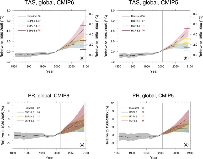
262                                                       C. Tebaldi et al.: Climate model projections from ScenarioMIP of CMIP6

Figure 4. Comparison of the three SSP-based scenarios updating three CMIP5-era RCPs with the corresponding CMIP5 output: SSP1-2.6,
SSP2-4.5 and SSP5-8.5 (a, c) can be compared to RCP2.6, RCP4.5 and RCP8.5 (b, d) for global average temperature change (a, b) and
global average precipitation change (c, d) (as a percentage of the baseline values, which are set to 1986–2005 for both ensembles). Indicators
along the right axis of the plots of temperature projections show constrained ranges at 2100, obtained by applying the method of Tokarska
et al. (2020). Note that, as in Fig. 1, the uncertainty bands in all figures are computed for anomalies with respect to the historical baseline
(1986–2005 in this case). Thus, the right axis of the global temperature plots, showing anomalies with respect to pre-industrial values, applies
to the ensemble means, not to the uncertainty bands, which would be narrowest over the 1850–1900 baseline, were they calculated using the
data from simulations over that period, rather than being registered to the new axis only on the basis of the offset. Figure A6 shows a more
direct comparison of the CMIP6 and CMIP5 ranges before and after the application of constraints at 2081–2100, and Table A6 lists those
ranges (and the unconstrained percent precipitation changes for the same comparisons) at 2041–2060 and 2081–2100.

0.46 (for the scenarios reaching 2.6 W m−2 ), 0.49 (for the               al., 2020) constrain the ensemble projections according to
4.5 W m−2 scenarios) and 0.67 ◦ C (for the 8.5 W m−2 scenar-              the evaluation of the ensemble historical behavior. All stud-
ios) more mean warming, while the upper end of the shading                ies find a strong correlation between the simulated warm-
for SSP5-8.5 reaches 1.5 ◦ C higher than the CMIP5 results                ing trends over the observed historical period and the warm-
(Table A6). The larger warming resulting from the CMIP6                   ing in SSP scenarios, which suggested constraining future
experiments is a combination of different forcings and the                warming using observed warming trends estimated from sev-
presence among the new ensemble of models with higher                     eral observational products, and all come to similar results.
climate sensitivities than the members of the previous gener-             Here, and in Table A6, we show how the 2081–2100 means
ations. The higher climate sensitivities in CMIP6 compared                for both CMIP5 and CMIP6 are changed as a result of
to CMIP5 (Meehl et al., 2020; Zelinka et al., 2020) become                applying constraints as in Tokarska et al. (2020). Also in
more critical for higher forcings, when the model response                Fig. A6, we show the same results but focus specifically on
is more highly correlated to its climate sensitivity, explaining          these 20-year means, before and after the application of the
the differential in the higher warming across the range of new            constraints. The resulting observationally constrained ranges
scenarios, with the largest difference evident for SSP5-8.5.              bring CMIP6 projections closer to both the raw CMIP5
   Several recent studies (Brunner et al., 2020; Liang et al.,            ranges and their constrained counterparts in both mean and
2020; Nijsse et al., 2020; Ribes et al., 2021; Tokarska et                spread (especially the upper bound). In other words, models

Earth Syst. Dynam., 12, 253–293, 2021                                                          https://doi.org/10.5194/esd-12-253-2021
C. Tebaldi et al.: Climate model projections from ScenarioMIP of CMIP6                                                     263

that project the most warming by the end of the century tend      pollution in the SSP3-7.0 pathway to very ambitious reduc-
to do the least well in reproducing historical warming trends     tions of air pollution in the SSP1-2.6, SSP1-1.9 and SSP5-8.5
for both ensembles, but the effect is much more pronounced        pathways (Rao et al., 2017). All the CMIP5 RCPs followed
for CMIP6 than CMIP5 models (see also Fig. A6). After con-        by comparison a more “middle-of-the-road” pollution policy
straints are applied, the difference in the mean changes by       path. Last, the effective radiative forcing levels reached by
2081–2100 is 0.29 for the two lower scenarios and 0.15 ◦ C        both sets of pathways can be different – depending on each
under SSP5-8.5/RCP8.5. The difference in the upper range          climate model processes – from their nominal AR5-SARF
under the latter scenario is reduced to 0.59 ◦ C.                 values labeling the pathway, usually obtained by running the
   Global precipitation projections follow temperature pro-       emission pathways through simple models, like using the
jections (O’Gorman et al., 2012), and therefore we see            Model for the Assessment of Greenhouse Gas Induced Cli-
(unconstrained) CMIP6 trajectories reaching higher percent        mate Change (MAGICC) in its AR5-consistent setup (Riahi
changes than CMIP5 of just below 1 %. Consistent with the         et al., 2017). A recent study with the EC-Earth model finds
relatively larger means, the spread of trajectories for indi-     that about half of the difference in warming by the end of
vidual scenarios, which combines internal variability with        the century when comparing CMIP5 RCPs and their updated
model uncertainty, is larger for the new models and scenar-       CMIP6 counterparts is due to difference in effective radia-
ios.                                                              tive forcings at 2100 of up to 1 W m−2 (Wyser et al., 2020).
   As mentioned, part of the differences described are due        Figure A7, adapted from Meinshausen et al. (2020), shows
to forcing differences between the corresponding scenar-          a breakdown of the comparison into the three main forcing
ios in CMIP5 and CMIP6. These are by design small in              agents among greenhouse gases (CO2 , CH4 and N2 O) from
terms of aggregate radiative forcing, when radiative forcing      which the significant differences in the composition can be
is defined as Intergovernmental Panel on Climate Change           assessed. Next to the AR5-consistent SARF time series, we
fifth Assessment Report (IPCC AR5)-consistent total global        also show effective radiative forcing ranges under the SSPs
stratospheric-adjusted radiative forcing (AR5-SARF). By           for the end of the 21st century for comparison using a newer
this measure of forcing, scenarios differ by less than 6 %        version of MAGICC (MAGICC7.3).
in 2100 for the SSP1-2.6/RCP2.6 pair, 5 % for the SSP2-              Here, we note that in an effort to make the compari-
4.5/RCP4.5 pair and around 0.3 % at 8.9 W m−2 for the             son more direct, CMIP5 RCP forcings are available to be
SSP5-8.5/RCP8.5 pair. Differences over the full pathway           run with CMIP6 models, and several modeling centers have
from 2015 to 2100 are below 15 %, 5 % and 4 %, respectively.      started – at the time of writing – these experiments, which
However, the literature in recent years has moved away from       have been added to the Tier 2 design of ScenarioMIP since
the AR5-SARF definition (in particular, Etminan et al., 2016;     the description in O’Neill et al. (2016). If enough models
see also implementation in Meinshausen et al., 2020) towards      contribute these results, a cleaner comparison of the effects
the use of effective radiative forcing (ERF), which differs       of the updated forcing pathways, controlling for the updated
from AR5-SARF in that it includes any non-temperature-            models’ effect, will be possible. Preliminary results with the
mediated feedbacks (see, e.g., Smith et al., 2020).               Canadian model, CanESM2, confirm the significant role of
   Given that CMIP5 and CMIP6 concentration pathways              higher radiative forcings found with EC-Earth.
differ with respect to their composition across gases and
other radiatively active species (Lurton et al., 2020, Fig. 1),   3.1.4   Scenarios and warming levels
whose respective ERFs can be very different despite a similar
AR5-SARF, the similarity between RCP and SSP scenarios            The ever-increasing attention to warming levels as policy
in terms of forcing deteriorates when moving away from an         targets, also due to the recognition that strong relations are
AR5-SARF definition. For example, in SSP5-8.5, the AR5-           found between them and a large set of impacts, motivates
SARF contribution of CH4 is by 2100 about 0.5 W m−2 lower         us to identify the time windows at which the new scenarios’
than in the CMIP5 RCP8.5 pathway. This is offset by the           global temperature trajectories reach 1.5, 2.0, 3.0, 4.0 and
difference in CO2 AR5-SARF, where SSP5-8.5 is around              5.0 ◦ C since 1850–1900. Table 1 shows the timing of first
0.5 W m−2 higher. In contrast, these compensating effects do      crossing of the thresholds by the ensemble average and the
not hold any longer when using ERF. In fact, because ERF is       5 %–95 % uncertainty range around that date. This is derived
higher than AR5-SARF for CO2 and even more so for CH4 ,           by computing the 5 %–95 % range for the ensemble of tra-
the 2100 radiative forcing levels after which both the RCP        jectories of GSAT and identifying the dates at which the up-
and SSP are named are not met precisely anymore when mea-         per and lower bounds of the range cross the threshold. The
sured by ERF. Another pronounced difference between the           range is computed by assuming a normal distribution for the
CMIP5 RCPs and the new generation of SSP-RCP scenarios            ensemble as the intermodel standard deviation multiplied by
is that the latter span a wider range of aerosol emissions and    1.64. Considering this range rather than the minimum and
corresponding forcings. The main reason for this difference       maximum bounds of the ensembles makes the estimates of
is a wider consideration of the possible development of air       the 5 %–95 % range more robust, especially for the lowest
pollution policies, ranging from major failure to address air     scenario (SSP1-1.9) for which we only rely on 13 models.

https://doi.org/10.5194/esd-12-253-2021                                              Earth Syst. Dynam., 12, 253–293, 2021
264                                                       C. Tebaldi et al.: Climate model projections from ScenarioMIP of CMIP6

Table 1. Times (best estimate and range – in square brackets – based on the 5 %–95 % range of the ensemble after smoothing the trajec-
tories by 11-year running means) at which various warming levels (defined as relative to 1850–1900) are reached according to simulations
following, from left to right, SSP1-1.9, SSP1-2.6, SSP2-4.5, SSP3-7.0 and SSP5-8.5. Crossing of these levels is defined by using anomalies
with respect to 1995–2014 for the model ensembles and adding the offset of 0.84 ◦ C to derive warming from pre-industrial values. We use a
common subset of 31 models for the Tier 1 scenarios and all available models (13) for SSP1-1.9, while Table A7 shows the result of using
all available models under each scenario. The number of models available under each scenario and the number of models reaching a given
warming level are shown in parentheses. However, the estimates are based on the ensemble means and ranges computed from all the models
considered (13 or 31 in this case), not just from the models that reach a given level. An estimate marked as “NA” is to be interpreted as “not
reaching that warming level by 2100”. In cases where the ensemble average remains below the warming level for the whole century, it is
possible for the central estimate to be NA, while the earlier time of the confidence interval is not, since it is determined by the warmer end of
the ensemble range.

                                        SSP1-1.9        SSP1-2.6        SSP2-4.5         SSP3-7.0         SSP5-8.5
                            1.5 ◦ C         2029            2028             2028             2028             2026
                                      [2021, NA]      [2020, NA]     [2020, 2047]     [2020, 2045]     [2020, 2040]
                                          (11/13)         (30/31)         (31/31)          (31/31)          (31/31)
                            2.0 ◦ C           NA            2064             2046             2043             2039
                                      [2036, NA]      [2032, NA]     [2032, 2082]     [2031, 2064]     [2030, 2055]
                                           (2/13)         (17/31)         (31/31)          (31/31)          (31/31)
                            3.0 ◦ C           NA             NA             2094             2069              2060
                                        [NA, NA]       [NA, NA]       [2058, NA]       [2052, NA]      [2048, 2083]
                                           (0/13)         (0/31)          (16/31)          (31/31)          (31/31)
                            4.0 ◦ C           NA             NA               NA             2091             2078
                                        [NA, NA]       [NA, NA]         [NA, NA]       [2071, NA]       [2062, NA]
                                           (0/13)         (0/31)           (1/31)          (17/31)          (27/31)
                            5.0 ◦ C           NA             NA               NA               NA             2094
                                        [NA, NA]       [NA, NA]         [NA, NA]       [2088, NA]       [2075, NA]
                                           (0/13)         (0/31)           (0/31)           (3/31)          (15/31)

The analysis is conducted after smoothing each of the in-                     The lowest warming level of 1.5 ◦ C from pre-industrial
dividual models’ time series by an 11-year running average                 values is reached on average between 2026 and 2028 across
to smooth interannual variability. The width of the intervals              SSP1-2.6, SSP2-4.5, SSP3-7.0 and SSP5-8.5 with largely
would change if constraints based on the observed warming                  overlapping confidence intervals that start from 2020 as the
trends were applied to the ensemble along the whole century                shortest waiting time and extend until 2046 at the latest un-
(as shown in Fig. 4 for the end of the century), but here the              der SSP2-4.5. Note, however, that the lower bound of the en-
unconstrained ensemble is used. The anomalies from 1850 to                 semble trajectories (determining the upper bound of the pro-
1900 are computed as described in Sect. 3.1.1 by calculating               jected years by which the level is reached) under SSP1-2.6
anomalies with respect to the historical baseline (1995–2014)              does not warm to 1.5 ◦ C for the whole century (the NA as the
and then adding the offset value of 0.84 ◦ C to minimize the               upper bound of the time period signifies “not reached”). The
effect of biases in the warming during the historical period               next level of 2.0 ◦ C is reached as soon as 13 years later by
of the different models. Note, however, that remaining dif-                the ensemble average under SSP5-8.5 and as late as 32 years
ferences between models and observations in the warming                    later under SSP1-2.6, a striking reminder of how different
trends over the period 2014 to present, and the effects of dif-            the pace of warming is in these scenarios. The confidence
ferences between observed and projected forcings, may still                intervals have similar lower bounds between 2030 and 2032
introduce biases in the crossing level estimates, likely biasing           and extend to 2077 for SSP2-4.5, while they are significantly
them low.                                                                  shorter for the higher scenarios (2064 and 2054 for SSP3-
   We first synthesize results from the experiments from                   7.0 and SSP5-8.5, respectively). The confidence intervals for
Tier 1, for which we extract a common subset of 31 models                  SSP1-2.6 do not reach any of the higher warming levels,
in order to make the threshold crossing estimates comparable               while by 2059 the ensemble average under SSP5-8.5 has al-
across scenarios (for completeness, we document in Table A7                ready warmed by 3 ◦ C. SSP3-7.0 takes 9 more years, while it
the behavior of all models available, which does not change                takes until 2092 for the ensemble average under SSP2-4.5
qualitatively the results that we are about to describe).                  to reach 3 ◦ C. Under this scenario, it is worth noting that
                                                                           only 21 out of 37 models reach that level. Only the ensem-

Earth Syst. Dynam., 12, 253–293, 2021                                                           https://doi.org/10.5194/esd-12-253-2021
C. Tebaldi et al.: Climate model projections from ScenarioMIP of CMIP6 265
ble means of the two higher scenarios reach 4 ◦ C, as early realization standard deviations. In the following, the phrase
as 2077 for SSP5-8.5 and 14 years later for SSP3-7.0. The “ensemble spread” is used, which has to be interpreted as
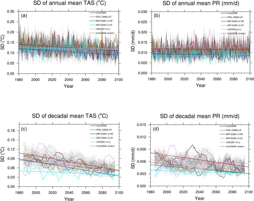
highest warming level considered of 5 ◦ C is only reached by the value of such standard deviation. Figure 5 shows the
the upper range of SSP3-7.0 (only four models out of 33), time evolution (over 1980–2100) of the ensemble spreads for
while more than half the models running SSP5-8.5 (21 out of global temperature and precipitation computed on an annual
39) reach that warming level in the last decade of the century basis (a and b) and after smoothing the individual time se-
(2094) as an ensemble average and as early as 2074 when the ries by an 11-year running mean (c and d). One of the mod-
warmer end of the ensemble range is considered. els, CanESM5, provides 50 ensemble members that we use
Only 13 models are available at the time of writing under to randomly select subsets of 10 members and form a back-
the lowest scenario specifically designed to meet the Paris ground “distribution” of the time series of ensemble spreads,
Agreement target of 1.5 ◦ C warming by the end of the cen- shown in gray in Fig. 5. This is not meant to provide a quanti-
tury. Of those, two remain below that target for the entire cen- tative assessment but rather a qualitative representation of the
tury, while others have a small overshoot of the target which variability of “10-member ensembles”, which is what most
was expected by design. The ensemble mean reaches 1.5 ◦ C models provide. When we compute trends for the time se-
already by 2029. The lower bound never crosses that level, ries of the temperature-ensemble spreads all show a negative
while the upper bound is already at 1.5 ◦ C currently, i.e., slope, indicating that the ensemble spread has a tendency to
by 2021 (as a reminder, CMIP6 future simulations start at narrow over time. In the case of the spread being computed
2015). In Table A8, a comparison of the CMIP5/CMIP6 three among annual values, only two of the models pass a signif-
corresponding scenarios (SSP1-2.6, SSP2-4.5 and SSP5-8.5 icance test at the 5 % level, while for decadal averages all
compared to RCP2.6, RCP4.5 and RCP8.5) for a slightly models show significantly decreasing spreads (significantly
larger ensemble of 36 CMIP6 models for which the three negative trends). Trends of the ensemble spreads for precip-
scenarios are available, and a CMIP5 ensemble of 29 mod- itation are non-significant for all models when the spread is
els, shows dates compatible with the warmer characteristics computed from annual values, while all are significantly neg-
of the CMIP6 models or scenarios. On average, the same tar- ative, indicating a decrease in the spread, when that is com-
get is reached from 3 to 9 years earlier by the CMIP6 ensem- puted from decadal means. This result appears robust for this
ble means compared to the CMIP5 ensemble means. A more small set of models, but confirmation with a larger number of
in-depth analysis than is in our scope is necessary to fully models providing sizable initial condition ensembles will be
characterize the causes of this acceleration. Here, we note important. Decreases in GSAT variability have however been
that the behavior of the CMIP6 ensemble means reflects the found in earlier studies (Huntingford et al., 2013; Brown et
use of unconstrained projections, with equal weight given to al., 2017) and attributed to reduced Equator-to-pole gradi-
high-climate-sensitivity models, which are often also those ents and reduced albedo variability due to the disappearance
less adherent to historical trends and that may show a faster of snow and sea ice. A deeper investigation of the sources
historical warming in the last decade or so than observed. In of changes in variability for both variables (which could also
addition, as we discussed in the previous section, even sce- tackle how much of the change in precipitation variability is
narios having the same AR5-SARF label see different forc- directly connected to that of GSAT and what other sources
ings at play. The result is to make the pace of warming faster, may be at play) is beyond our scope but will be facilitated
and, in several cases, a target that was not reached by the by the availability of these CMIP6 IC ensembles in addition
CMIP5 models under a given scenario is instead reached by to the already-well-studied CMIP5-era large IC ensembles
the CMIP6 ensemble under the corresponding scenario. For (Deser et al., 2020).
example, 2.0 ◦ C under SSP1-2.6 is reached in mean in 2056, After detrending the values, we compare the distribution
while it was reached only by the upper bound (by 2040) un- of the ensemble spreads for an individual model to that of
der RCP2.6; at the opposite end, 5.0 ◦ C was reached only by other models in order to assess if models produce ensem-
the upper bound (in 2083) under RCP8.5, while it is reached bles with spreads that are significantly different. We use a
by the ensemble mean in 2093 under SSP5-8.5. Kolmogorov–Smirnov test (at 5 % level) which measures dif-
ferences in distribution. For several pairs of models, ensem-
ble spreads based on annual values turn out to be indistin-
3.2 Climate projections from ScenarioMIP Tier 2 guishable: for temperature, CanESM5 ensemble spread is not
simulations significantly different from those of the MPI-ESM model at
3.2.1 SSP3-7.0 initial condition ensembles low resolution and those of the UKESM1 model. The lat-
ter in turn has an ensemble spread that is not different from
Five models (CanESM5, IPSL-CM6A-LR, MPI-ESM1-2- that of the IPSL-CM model. For precipitation, CanESM5 and
HR, MPI-ESM1-2-LR and UKESM1) contributed at least IPSL-CM produce comparable spreads, as do the two MPI-
10 initial condition (IC) ensemble members under SSP3- ESM models, and the MPI-ESM at low resolution compared
7.0. We focus here on the behavior of the ensemble spread to UKESM1. When we test the spreads of decadal means,
over the 21st century, as measured by the values of the inter- all models appear significantly different from one another.
https://doi.org/10.5194/esd-12-253-2021 Earth Syst. Dynam., 12, 253–293, 2021You can also read