Satellite soil moisture data assimilation impacts on modeling weather variables and ozone in the southeastern US - Part 1: An overview - Recent
←
→
Page content transcription
If your browser does not render page correctly, please read the page content below
Atmos. Chem. Phys., 21, 11013–11040, 2021
https://doi.org/10.5194/acp-21-11013-2021
© Author(s) 2021. This work is distributed under
the Creative Commons Attribution 4.0 License.

Satellite soil moisture data assimilation impacts on modeling
weather variables and ozone in the southeastern US – Part 1:
An overview
Min Huang1 , James H. Crawford2 , Joshua P. DiGangi2 , Gregory R. Carmichael3 , Kevin W. Bowman4 ,
Sujay V. Kumar5 , and Xiwu Zhan6
1 College of Science, George Mason University, Fairfax, VA, USA
2 NASA   Langley Research Center, Hampton, VA, USA
3 College of Engineering, University of Iowa, Iowa City, IA, USA
4 Jet Propulsion Laboratory, California Institute of Technology, Pasadena, CA, USA
5 NASA Goddard Space Flight Center, Greenbelt, MD, USA
6 NOAA National Environmental Satellite, Data, and Information Service, College Park, MD, USA

Correspondence: Min Huang (mhuang10@gmu.edu)

Received: 22 May 2020 – Discussion started: 7 August 2020
Revised: 27 April 2021 – Accepted: 11 May 2021 – Published: 21 July 2021

Abstract. This study evaluates the impact of satellite soil     ical production of O3 from lightning and other emissions.
moisture (SM) data assimilation (DA) on regional weather        Case studies during airborne field campaigns suggest that
and ozone (O3 ) modeling over the southeastern US dur-          the DA improved the model treatment of convective trans-
ing the summer. Satellite SM data are assimilated into the      port and/or lightning production. In the cases that the DA
Noah land surface model using an ensemble Kalman fil-           improved the modeled SM, weather fields, and some O3 -
ter approach within National Aeronautics and Space Ad-          related processes, its influences on the model’s O3 perfor-
ministration’s Land Information System framework, which         mance at various altitudes are not always as desirable. This
is semicoupled with the Weather Research and Forecasting        is in part due to the uncertainty in the model’s key chemical
model with online Chemistry (WRF-Chem; standard version         inputs, such as anthropogenic emissions, and the model rep-
3.9.1.1). The DA impacts on the model performance of SM,        resentation of stratosphere–troposphere exchanges. This can
weather states, and energy fluxes show strong spatiotem-        also be attributable to shortcomings in model parameteriza-
poral variability. Dense vegetation and water use from hu-      tions (e.g., chemical mechanism, natural emission, photoly-
man activities unaccounted for in the modeling system are       sis and deposition schemes), including those related to rep-
among the factors impacting the effectiveness of the DA.        resenting water availability impacts. This study also shows
The daytime surface O3 responses to the DA can largely          that the WRF-Chem upper tropospheric O3 response to the
be explained by the temperature-driven changes in biogenic      DA has comparable magnitudes with its response to the es-
emissions of volatile organic compounds and soil nitric ox-     timated US anthropogenic emission changes within 2 years.
ide, chemical reaction rates, and dry deposition velocities.    As reductions in anthropogenic emissions in North America
On a near-biweekly timescale, the DA modified the mean          would benefit the mitigation of O3 pollution in its downwind
daytime and daily maximum 8 h average surface O3 by up          regions, this analysis highlights the important role of SM in
to 2–3 ppbv, with the maximum impacts occurring in areas        quantifying air pollutants’ source–receptor relationships be-
where daytime surface air temperature most strongly (i.e.,      tween the US and its downwind areas. It also emphasizes
by ∼ 2 K) responded to the DA. The DA impacted WRF-             that using up-to-date anthropogenic emissions is necessary
Chem upper tropospheric O3 (e.g., for its daytime-mean, by      for accurately assessing the DA impacts on the model per-
up to 1–1.5 ppbv) partially via altering the transport of O3    formance of O3 and other pollutants over a broad region.
and its precursors from other places as well as in situ chem-   This work will be followed by a Noah-Multiparameterization

Published by Copernicus Publications on behalf of the European Geosciences Union.
11014                                            M. Huang et al.: Soil moisture, weather, and ozone in the southeastern US

(with dynamic vegetation)-based study over the southeast-         posphere. They are active throughout the year and relatively
ern US, in which selected processes including photosynthesis      weaker during the summer. Convection, often associated
and O3 dry deposition will be the foci.                           with thunderstorms and lightning, is a dominant mechanism
                                                                  of exporting pollution in the summertime (e.g., Dickerson et
                                                                  al., 1987; Hess, 2005; Brown-Steiner and Hess, 2011; Barth
                                                                  et al., 2012). During North American summers, upper tropo-
1   Introduction                                                  spheric anticyclones trap convective outflows and promote in
                                                                  situ O3 production from lightning and other emissions (e.g.,
Tropospheric ozone (O3 ) is a central component of tro-           Li et al., 2005; Cooper et al., 2006, 2007, 2009). It has also
pospheric oxidation chemistry, with atmospheric lifetimes         been shown that stratospheric O3 intrusions are often associ-
ranging from hours within polluted boundary layer to weeks        ated with cold frontal passages and convection (e.g., Pan et
in the free troposphere (Stevenson et al., 2006; Cooper et        al., 2014; Ott et al., 2016).
al., 2014; Monks et al., 2015). Ground-level O3 is a US              On a wide range of spatial and temporal scales, atmo-
Environmental Protection Agency (EPA) criteria air pollu-         spheric weather and composition interact with land surface
tant which harms human health and imposes threat to veg-          conditions (e.g., soil and vegetation states, topography, and
etation and sensitive ecosystems, and such impacts can be         land use and land cover, LULC), which can be altered by
strongly linked or/and combined with other stresses, such as      various human activities and/or natural disturbances such as
heat, aridity, soil nutrients, diseases, and non-O3 air pollu-    urbanization, deforestation, irrigation, and natural disasters
tants (e.g., Harlan and Ruddell, 2011; Avnery et al., 2011;       (e.g., Betts et al., 1996; Kelly and Mapes, 2010; Taylor et
World Health Organization, 2013; Fishman et al., 2014; Lap-       al., 2012; Collow et al., 2014; Guillod et al., 2015; Tuttle
ina et al., 2014; Cohen et al., 2017; Fleming et al., 2018;       and Salvucci, 2016; Cioni and Hohenegger, 2017; Fast et
Mills et al., 2018a, b). Across the world, various metrics have   al., 2019; Schneider et al., 2019). As a key land variable, soil
been used to assess surface O3 impacts (Lefohn et al., 2018).     moisture (SM) influences the atmosphere via evapotranspi-
In October 2015, the US primary (to protect human health)         ration, including evaporation from bare soil and plant tran-
and secondary (to protect public welfare including vegeta-        spiration. The SM–atmosphere coupling strengths are over-
tion and sensitive ecosystems) National Ambient Air Qual-         all strong over transitional climate zones (i.e., the regions
ity Standards for ground-level O3 , in the format of the daily    between humid and arid climates) where evapotranspiration
maximum 8 h-average (MDA8), were revised to 70 parts per          is moderately high and constrained by SM (e.g., Koster et
billion by volume (ppbv; US Federal Register, 2015). Under-       al., 2004, 2006; Seneviratne et al., 2010; Dirmeyer, 2011;
standing the connections between weather patterns and sur-        Miralles et al., 2012; Gevaert et al., 2018). The southeast-
face O3 , as well as their combined impacts on human and          ern US includes large areas of transitional climate zones,
ecosystem health under the changing climate, is important         whose geographical boundaries vary temporally (e.g., Guo
for the development of anthropogenic emission controls that       and Dirmeyer, 2013; Dirmeyer et al., 2013). Soil moisture
are strong enough to meet target O3 air quality standards         and other land variables are currently measurable from space.
(Jacob and Winner, 2009; Doherty et al., 2013; Coates et          It has been shown in a number of scientific and operational
al., 2016; Lin et al., 2017).                                     applications that satellite SM data assimilation (DA) impacts
   Ozone aloft is more conducive to rapid long-range trans-       model skill of atmospheric weather states and energy fluxes
port to influence surface air quality in downwind regions         (e.g., Mahfouf, 2010; de Rosnay et al., 2013; Santanello et
(e.g., Zhang et al., 2008; Fiore et al., 2009; Hemispheric        al., 2016; Yin and Zhan, 2018). An effort began recently
Transport of Air Pollution, HTAP, 2010, and references            to evaluate the impacts of satellite SM DA on short-term
therein; Huang et al., 2010, 2013, 2017a; Doherty, 2015). In      regional-scale air quality modeling. Based on case studies
the upper troposphere–lower stratosphere regions, O3 as well      in East Asia, such effects are shown to vary in space and
as water vapor is particularly important to climate (Solomon      time, partially dependent on surface properties (e.g., vegeta-
et al., 2010; Shindell et al., 2012; Stevenson et al., 2013;      tion density and terrain) and synoptic weather patterns. Also,
Bowman et al., 2013; Intergovernmental Panel on Climate           the SM DA impacts on model performance can be compli-
Change, 2013; Rap et al., 2015; Harris et al., 2015). Ozone       cated by other sources of model error, such as the uncer-
variability in the free troposphere can be strongly affected      tainty of the models’ chemical inputs including emissions
by stratospheric air and transport of O3 that is produced at      and chemical initial and lateral boundary conditions (Huang
other places of the troposphere, as well as in situ chemi-        et al., 2018).
cal production from O3 precursors including nitrogen oxides          This study extends the work by Huang et al. (2018) to
(NOx , namely nitric oxide, NO, and nitrogen oxide, NO2 ),        the southeastern US during intensive field campaign peri-
carbon monoxide (CO), methane, and non-methane volatile           ods in the summer convective season. Modified from the
organic compounds (VOCs). Midlatitude cyclones are ma-            approach used in Huang et al. (2018), we assimilate satel-
jor mechanisms of venting boundary layer constituents, in-        lite SM into the Noah land surface model (LSM) within
cluding O3 and its precursors, to the middle and upper tro-       National Aeronautics and Space Administration (NASA)’s

Atmos. Chem. Phys., 21, 11013–11040, 2021                                         https://doi.org/10.5194/acp-21-11013-2021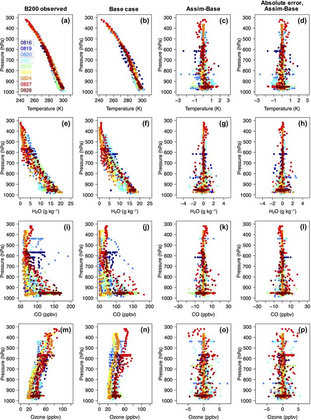
M. Huang et al.: Soil moisture, weather, and ozone in the southeastern US                                                 11015

Land Information System (LIS), which is semicoupled with          equilibrated land conditions (details in Sect. S1 in the Sup-
the Weather Research and Forecasting model with online            plement). Consistent model grids and geographical inputs of
Chemistry (WRF-Chem). The term “semicoupled” indicates            the Noah LSM were used in the offline LIS and all WRF-
that the SM DA within LIS influences WRF-Chem’s land ini-         Chem simulations. Specifically, topography, time-varying
tial conditions. Atmospheric states and energy fluxes from        green vegetation fraction, LULC type, and soil texture type
the no-DA and DA cases are compared with surface, aircraft,       inputs were based on the Shuttle Radar Topography Mission
and satellite observations during selected field campaign pe-     Global Coverage-30 version 2.0, Copernicus Global Land
riods. The WRF-Chem results are also compared with the            Service, the International Geosphere-Biosphere Programme-
chemical fields of the Copernicus Atmosphere Monitoring           modified Moderate Resolution Imaging Spectroradiometer
Service (CAMS), which serves as the chemical initial/lateral      (Fig. 1a–c), and the State Soil Geographic (Fig. S1, upper,
boundary condition model of WRF-Chem. Other sources of            in the Supplement; Miller and White, 1998) datasets, respec-
errors in WRF-Chem simulated O3 are identified by a WRF-          tively.
Chem emission sensitivity simulation and the stratospheric           Successful, valid retrievals of morning-time SM (version 2
O3 tracer output from the Geophysical Fluid Dynamics Lab-         of the 9 km enhanced product, generated using baseline re-
oratory (GFDL)’s Atmospheric Model, version 4 (AM4).              trieval algorithm) from NASA’s Soil Moisture Active Pas-
The modeling and SM DA approaches as well as evaluation           sive (SMAP; Entekhabi et al., 2010) L-band polarimetric
datasets are first introduced in Sect. 2. Section 3 starts with   radiometer were assimilated into Noah within LIS. SMAP
an overview of the synoptic and drought conditions during         provides global coverage of surface (i.e., the top 5 cm of
the study periods (Sect. 3.1), followed by discussions on the     the soil column) SM within 2–3 d along its morning orbit
model responses to satellite SM DA. The SM DA impacts             (∼ 06:00 local time crossing) with the ground track repeat-
on O3 export from the US and the potential impacts on sur-        ing in 8 d. Compared to its predecessors that take measure-
face O3 in regions downwind of the US are included in the         ments at higher frequencies, SMAP has a higher penetration
discussions. Results during a summer 2016 field campaign          depth for SM retrievals and lower attenuation in the presence
and a summer 2013 campaign are covered in Sect. 3.2–3.3           of vegetation. Evaluation of SMAP data over North America
and 3.4, respectively. Section 4 summarizes key results from      with in situ and LSM output suggests better data quality over
its previous sections, discusses their implications, and pro-     flat and less forested regions (Pan et al., 2016), and previous
vides suggestions on future work.                                 studies have demonstrated that the SMAP DA improvements
                                                                  on weather variables are more distinguishable over regions
                                                                  with sparse vegetation (e.g., Huang et al., 2018; Yin and
2     Methods                                                     Zhan, 2018). Before the DA, SMAP data were re-projected
                                                                  to the model grid and bias correction was applied via match-
2.1    Modeling and SM DA approaches                              ing the means and standard deviations of the Noah LSM and
                                                                  SMAP data for each grid (de Rosnay et al., 2013; Huang et
This study focuses on a summer southeastern US deploy-            al., 2018; Yin and Zhan, 2018) during August 2015–2019.
ment (16–28 August 2016) of the Atmospheric Carbon and            Such bias correction reduced the dynamic ranges of SM from
Transport (ACT)-America campaign (https://act-america.            the original SMAP retrievals. The Global Modeling and As-
larc.nasa.gov, last access: 14 March 2021). One goal of this      similation Office (GMAO) ensemble Kalman filter approach
campaign is to study atmospheric transport of trace gases.        embedded in LIS was applied, with the ensemble size of
Three WRF-Chem full-chemistry simulations (i.e., “base”,          20. Perturbation attributes of state variables (Noah SM) and
“assim”, and “NEI14” in Table 1) were conducted through-          meteorological forcing variables (radiation and precipitation)
out this campaign on a 63 vertical layer, 12 km × 12 km           were based on default settings of LIS derived from Kumar at
(209 × 139 grids) horizontal-resolution Lambert conformal         al. (2009).
grid centered at 33.5◦ N, 87.5◦ W (Fig. 1a–c). To help con-          All WRF-Chem cases, except the minus001 case, were
firm surface SM impacts on atmospheric conditions, a com-         started on 13 August 2016. Atmospheric meteorological ini-
plementary simulation “minus001” was also conducted in the        tial and lateral boundary conditions were downscaled from
same model grid, only for selected events during this cam-        the 3-hourly, 32 km North American Regional Reanalysis
paign (Table 1). Trace gases and aerosols were simulated si-      (NARR). Consistent with NARR, the WRF-Chem model
multaneously and interactively with the meteorological fields     top was set at 100 hPa, slightly above the climatological
using the standard version 3.9.1.1 of WRF-Chem (Grell et          tropopause heights for the study region and month. The
al., 2005).                                                       0.083◦ × 0.083◦ National Centers for Environmental Predic-
   Version 3.6 of the widely used, four-soil-layer Noah LSM       tion (NCEP) daily sea surface temperature (SST) reanalysis
(Chen and Dudhia, 2001) within LIS (Kumar et al., 2006)           product was used as an additional WRF forcing. Chemical
version 7.1rp8 served as the land component of the model-         initial and lateral boundary conditions for major chemical
ing/DA system used. An offline Noah simulation was per-           species were downscaled from the 6-hourly, 0.4◦ ×0.4◦ ×60-
formed within LIS prior to all WRF-Chem simulations for           level CAMS. Surface O3 from CAMS is positively biased

https://doi.org/10.5194/acp-21-11013-2021                                       Atmos. Chem. Phys., 21, 11013–11040, 2021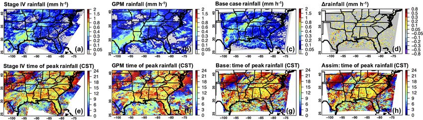
11016 M. Huang et al.: Soil moisture, weather, and ozone in the southeastern US
Table 1. Summary of WRF-Chem simulations conducted in this study.
Case Horizontal/vertical Analyzed period Assimilated SM data Anthropogenic
name resolutions (field campaign) (version; resolution) emission inputs for
various chemical species
Base none
Assim 16–28 August 2016 SMAP enhanced passive NEI 2016 beta
12 km/63 layer (ACT-America) (version 2; 9 km)
NEI14 none NEI 2014
Minus001 20 and 27 August 2016 none, surface SM initial conditions
(ACT-America) reduced uniformly by 0.01 m3 m−3 NEI 2016 beta
across the domain
SEACf 12–24 August 2013 none
25 km/27 layer NEI 2014
SEACa (SEAC4 RS) ESA CCI passive (version 04.5; 0.25◦ )
Acronyms are given as follows. ACT: Atmospheric Carbon and Transport; ESA CCI: European Space Agency Climate Change Initiative; NEI: National Emission
Inventory; SEAC4 RS: Studies of Emissions and Atmospheric Composition, Clouds and Climate Coupling by Regional Surveys; SM: soil moisture; SMAP: Soil Moisture
Active Passive; WRF-Chem: Weather Research and Forecasting model with online Chemistry.
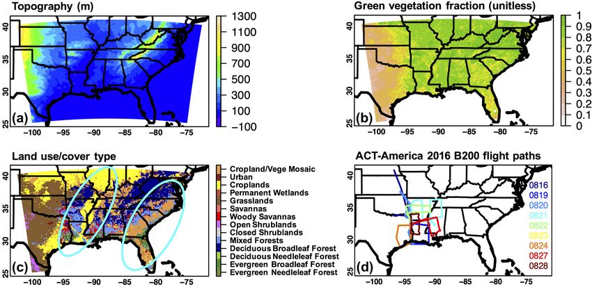
Figure 1. (a) Terrain heights, (b) August 2016 green vegetation fraction, and (c) grid-dominant land use–cover categories used in the 12 km
LIS/WRF-Chem simulations. (d) B-200 flight paths in the southeastern US during the 2016 ACT-America campaign. Cyan-blue circles in (c)
denote the approximate locations of areas with high irrigation water use based on literature. Similar model domains and consistent sources
of geographical inputs and meteorological forcings were used in 12 and 25 km LIS/WRF-Chem simulations.
over the eastern US referring to various observations, but et al., 2020) and its stratospheric O3 tracer, which have been
major chemical species in the free troposphere are overall applied to other O3 studies (e.g., Zhang et al., 2020). Since
successfully reproduced (e.g., Huijnen et al., 2020; Wang the second day of the simulation period, chemical initial con-
et al., 2020). As WRF-Chem only has tropospheric chem- ditions were cycled from the chemical fields of the previ-
istry, the lack of dynamic chemical upper boundary con- ous day’s simulation. Atmospheric meteorological and land
ditions is expected to introduce biases in the modeled O3 fields were reinitialized every day at 00:00 UTC with NARR
throughout the troposphere, and such biases depend on the and the previous day’s no-DA or DA LIS outputs, respec-
distribution of model vertical layers, as well as the length of tively. Each day’s simulation was recorded hourly at 00:00
the simulation. To determine how this limitation of WRF- (minute:second) through the following 30 h, forced by tem-
Chem affects its O3 performance, we used the outputs (3- porally constant SST as the diurnal variation of the sea sur-
hourly, 1◦ × 1.25◦ × 49-level) from GFDL’s AM4 (Horowitz face is typically smaller than land on large scales. Each day’s
Atmos. Chem. Phys., 21, 11013–11040, 2021 https://doi.org/10.5194/acp-21-11013-2021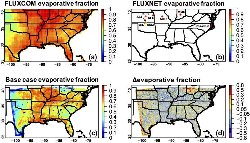
M. Huang et al.: Soil moisture, weather, and ozone in the southeastern US                                                   11017

WRF-Chem meteorological outputs served as the forcings of          both intra-cloud and cloud-to-ground flashes, 125 mol of
the no-DA and DA LIS simulations, which produced land              NO was emitted per flash, close to the estimates in several
initial conditions for the next day’s WRF-Chem simulations.        studies for the US (e.g., Pollack et al., 2016; Bucsela et
The model output > 6 h since each day’s initialization was         al., 2019). The passive lightning NOx tracer was imple-
analyzed for the period of 16–28 August 2016.                      mented, which experienced atmospheric transport but not
   In all WRF-Chem simulations, key physics options ap-            chemical reactions. Anthropogenic emissions in the base,
plied include the local Mellor–Yamada–Nakanishi–Niino              assim, and minus001 simulations (Table 1) were based on
planetary boundary layer (PBL) scheme along with its               US EPA’s National Emission inventory (NEI) 2016 beta,
matching surface layer scheme (Nakanishi and Niino, 2009),         and NEI 2014 was used in the NEI14 simulation. The
the Rapid Radiative Transfer Model short- and long-                differences between NEI 2016 beta and earlier versions
wave radiation schemes (Iacono et al., 2008), the Morri-           of NEIs, such as NEI 2014 and 2011, are summarized
son double-moment microphysics, which predicts the mass            at http://views.cira.colostate.edu/wiki/wiki/10197/inventory-
and number concentrations of hydrometeor species (Mor-             collaborative-2016beta-emissions-modeling-
rison et al., 2009), and the Grell–Freitas scale-aware cu-         platform (last access: 27 March 2020), for various chemical
mulus scheme (Grell and Freitas, 2014), which has also             species. Anthropogenic emissions of O3 precursors are
been implemented in the GMAO GEOS-Forward Process-                 lower in NEI 2016 beta than in NEI 2014 (by < 20 % for key
ing system (https://gmao.gsfc.nasa.gov/news/geos_system_           species) as well as NEI 2011, in which NOx emissions may
news/2020/GEOS_FP_upgrade_5_25_1.php, last access: 14              be positively biased for 2013 (Travis et al., 2016). These dif-
March 2021). Chemistry-related configurations are the              ferences are qualitatively consistent with the observed trends
Carbon-Bond Mechanism version Z (Zaveri and Peters,                of surface air pollutants (https://www.epa.gov/air-trends,
1999) gas-phase chemical mechanism and the eight-bin sec-          last access: 27 March 2020).
tional Model for Simulating Aerosol Interactions and Chem-            Chemical loss via dry deposition (i.e., dry deposition ve-
istry (MOSAIC; Zaveri et al., 2008), including aqueous             locity vd multiplied by surface concentration) was calculated
chemistry for resolved clouds. Both aerosol direct and indi-       based on the widely used Wesely scheme (Wesely, 1989; de-
rect effects were enabled in all simulations.                      tails in Sect. S2). This scheme defines vd as the reciprocal
   Daily biomass burning emissions came from the Quick             of the sum of aerodynamic resistance, quasi-laminar sub-
Fire Emissions Dataset (Darmenov and da Silva, 2015) ver-          layer resistance, and surface resistance. Over the land, sur-
sion 2.5r1, and plume rise with a recent bug fix (suggested        face resistance, the major component of vd , is classified into
by Ravan Ahmadov, NOAA/ESRL, in August 2019) was                   stomatal–mesophyll and several other resistance terms. Sur-
applied. Emissions of biogenic VOCs and soil NO were               face resistance is usually strongly affected by its stomatal–
computed online (i.e., driven by the WRF meteorology)              mesophyll resistance term which in the Wesely scheme is
using the Model of Emissions of Gases and Aerosols from            expressed as season- and LULC-dependent constants, which
Nature (MEGAN; Guenther et al., 2006). It has been shown           are subject to large uncertainty, being adjusted by surface
that MEGAN may overpredict biogenic VOC emissions                  temperature and radiation. This contrasts with some other
over the study regions and tends to underpredict soil NO           approaches which also account for the influences of SM,
emissions, especially in high-temperature (i.e., > 30 ◦ C)         vapor pressure deficit (VPD), and vegetation density in ad-
agricultural regions (e.g., Oikawa et al., 2015; Huang et          justing these constants and which couple stomatal resistance
al., 2017b, and references therein). Important sources of          with photosynthesis. For calculating the other surface resis-
uncertainty include the following: (1) there is uncertainty        tance terms, prescribed season- and LULC-dependent con-
in MEGAN’s land and meteorological inputs, including               stants are used in the Wesely scheme, adjusted by environ-
surface temperature and radiation fields from WRF; and             mental variables including surface wetness, radiation, and
(2) drought influences on these emissions are not well             temperature, whereas in other existing schemes, impacts of
understood and represented in MEGAN, and such influences           friction velocity and vegetation density are also considered
include biogenic VOC emissions being enhanced, reduced,            (e.g., Charusombat et al., 2010; Park et al., 2014; Val Mar-
or terminated during various stages of droughts. Specifically,     tin et al., 2014; Wu et al., 2018; Mills et al., 2018b; Anav
at the early stage of droughts when plants still have sufficient   et al., 2018; Wong et al., 2019; Clifton et al., 2020, and ref-
reserved carbon resources, dry conditions may promote              erences therein). Aerodynamic resistance and quasi-laminar
these emissions via enhancing leaf temperature. Persistent         resistance are both sensitive to surface properties such as sur-
droughts will terminate biogenic VOC emissions after the           face roughness.
reserved carbon resources are consumed (e.g., Pegoraro                This paper also briefly discusses in Sect. 3.4 some re-
et al., 2004; Bonn et al., 2019). Cloud-top-height-based           sults from two WRF-Chem simulations (i.e., “SEACf” and
lightning parameterization was applied (Wong et al., 2013).        “SEACa” in Table 1) during the 2013 Studies of Emissions
The intra-cloud to cloud-to-ground flash ratio was based on        and Atmospheric Composition, Clouds and Climate Cou-
climatology (Boccippio et al., 2001), and lightning NO was         pling by Regional Surveys (SEAC4 RS; Toon et al., 2016;
distributed using vertical profiles in Ott et al. (2010). For      https://espo.nasa.gov/home/seac4rs/content/SEAC4RS, last

https://doi.org/10.5194/acp-21-11013-2021                                        Atmos. Chem. Phys., 21, 11013–11040, 2021
11018                                            M. Huang et al.: Soil moisture, weather, and ozone in the southeastern US

access: 14 March 2021) campaign. SEAC4 RS studies the at-         on 16, 20, and 21 August 2016 sampled the air under stormy
tribution and quantification of pollutants and their distribu-    weather conditions, whereas the other flights were conducted
tions as a result of deep convection. These simulations were      under fair weather conditions. We used meteorological as
conducted on a 27 vertical layer, 25 km × 25 km (99 × 67          well as collocated O3 and CO measurements collected on
grids) horizontal-resolution Lambert conformal grid, also         the B-200 to evaluate our WRF-Chem simulations. The O3
centered at 33.5◦ N, 87.5◦ W. Their LSM and inputs, WRF           mixing ratio measurements using the differential ultravio-
physics and chemistry configurations were the same as those       let absorption has a 5 ppbv uncertainty (Bertschi and Jaffe,
used in the 12 km cases described above. In SEACa, we as-         2005), and the CO mixing ratio was measured with an un-
similated successfully retrieved, daily SM from version 04.5      certainty of 10 ppbv, using a Picarro analyzer which is based
of the European Space Agency Climate Change Initiative            on wavelength-scanned cavity ring down spectroscopy (Kar-
project (ESA CCI) SM product (Gruber et al., 2019), de-           ion et al., 2013). We used the weather and trace gas ob-
veloped on a 0.25◦ × 0.25◦ horizontal-resolution grid based       servations averaged in 1 min intervals (version R1, released
on measurements from passive satellite sensors. The assim-        in November 2020) for model evaluation, as they repre-
ilated CCI SM data were re-projected to the model grid and        sent atmospheric conditions on comparable spatial scales to
bias-corrected based on the climatology of Noah and CCI           the model. Ozone and CO measurements with O3 /CO >
SM during August 1999–2018. These simulations were eval-          1.25 mol mol−1 (Travis et al., 2016) are assumed to be in-
uated with SEAC4 RS aircraft chemical observations, which         fluenced by fresh stratospheric intrusions and were excluded
were richer than those collected during ACT-America in            in our analysis. This approach, however, was rather arbitrary
terms of the diversity of measured reactive chemical com-         and may not have excluded air that had an aged stratospheric
pounds (Sect. 2.2.1). Such comparisons help evaluate the          origin or mixtures of air with different origins.
emissions of O3 precursors from various (e.g., NEI 2014 an-          Aircraft (NASA DC-8) in situ measurements of CO,
thropogenic, lightning, and biogenic) sources as well as how      NO2 , and formaldehyde (HCHO) from the surface to ∼
the model representation of land–atmosphere interactions af-      200 hPa during six SEAC4 RS daytime (i.e., within 13:00–
fects such emission assessments.                                  23:00 UTC, local time +6), 8–10 h science flights in Au-
   The model horizontal resolutions of 12 and 25 km were          gust 2013 were compared with our WRF-Chem simula-
set to be close to the assimilated satellite SM products to       tions. The CO mixing ratio was measured using the tun-
minimize the horizontal representation errors. At these res-      able diode laser spectroscopy technique, with an uncertainty
olutions, land surface heterogeneity and fine-scale processes     of 5 % or 5 ppbv. The NO2 measurements were made by
(e.g., cloud formation and turbulent mixing) may not be real-     two teams, based on thermal dissociation laser-induced flu-
istically represented. Cloud-top-height-based lightning emis-     orescence and chemiluminescence methods, with an uncer-
sions and SM–precipitation feedbacks can be highly depen-         tainty of ±5 % and (0.030 ppbv +7 %), respectively. Two
dent on convective parameterizations (e.g., Hohenegger et         other teams took the HCHO measurements, using a compact
al., 2009; Wong et al., 2013; Taylor et al., 2013). Addressing    atmospheric multispecies spectrometer and the laser-induced
shortcomings of convective parameterizations in simulations       fluorescence technique, with the uncertainty of ±4 % and
at these scales is still in strong need. Performing convection-   (0.010 ppbv ±10 %), respectively. Aircraft data averaged
permitting simulations with assimilation of downscaled mi-        in 1 min intervals (version R7, released in November
crowave SM or/and high-resolution thermal-infrared-based          2018) were used, with the biomass-burning-affected samples
SM (e.g., 2–8 km from the Geostationary Operational Envi-         (acetonitrile > 0.2 ppbv) and CO from fresh-stratospheric-
ronmental Satellite) for cloudless conditions should also be      intrusion-affected air (O3 /CO > 1.25 mol mol−1 ) excluded.
experimented on in the future.
                                                                  2.2.2   Ground-based measurements
2.2     Evaluation datasets
                                                                  WRF-Chem results were evaluated by various surface me-
2.2.1    Aircraft in situ measurements during                     teorological and chemical observations. These include the
         ACT-America and SEAC4 RS                                 following: (1) SM values observed at ∼ 5 and ∼ 10 cm be-
                                                                  low the surface, which were measured at various sites within
During the 2016 ACT-America deployment, the NASA B-               the Soil Climate Analysis Network (SCAN), were down-
200 aircraft took meteorological and trace gas measurements       loaded from the International Soil Moisture Network (Dorigo
in the southeastern US from the surface to ∼ 300 hPa on 9 d.      et al., 2011) and screened by quality flags before being used.
Different line colors in Fig. 1d denote individual flight paths   (2) Surface air temperature (T2), relative humidity (RH; de-
during this period. These flights were conducted under dif-       rived from the original dew point and air temperature data),
ferent weather conditions during the daytime (i.e., within        and wind speed (WS) from the NCEP Global Surface Ob-
14:00–23:00 UTC, local time +6), with durations of 4–             servational Weather Data were utilized. (3) Half-hourly or
9 h (https://www-air.larc.nasa.gov/missions/ACT-America/          hourly latent and sensible heat fluxes measured using the
reports.2019/index.html, last access: 14 March 2021). Flights     eddy covariance method at eight sites within the FLUXNET

Atmos. Chem. Phys., 21, 11013–11040, 2021                                         https://doi.org/10.5194/acp-21-11013-2021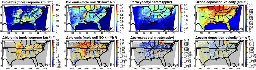
M. Huang et al.: Soil moisture, weather, and ozone in the southeastern US                                                   11019

network were used. Latent and sensible heat fluxes from this       tems from the Gulf of Mexico (https://www.ncdc.noaa.gov/
network exhibited mean errors of −5.2 % and −1.7 %, re-            sotc/synoptic/201608, last access: 14 March 2021). Temper-
spectively (Schmidt et al., 2012). We only analyzed the mod-       atures were consequently lower than normal in these regions.
eled energy fluxes at the sites where the model-based LULC         Contrastingly, controlled by the Bermuda High, more fre-
classifications are realistic. A 0.5◦ × 0.5◦ , daily FLUXCOM       quent air stagnation and warmer- and drier-than-normal con-
product was also utilized, which merges FLUXNET data               ditions affected multiple Atlantic states. Opposite hydrolog-
with machine learning approaches, remote sensing, and me-          ical anomalies were recorded during August 2016 and Au-
teorological data. Over North America, it is estimated that        gust 2013 for the Southern Great Plain and Atlantic regions
latent and sensible heat fluxes from this FLUXCOM prod-            (Fig. S2, left).
uct are associated with ∼ 12 % and ∼ 13 % of uncertainty,             The anomalies in synoptic patterns and drought conditions
respectively (Jung et al., 2019). (4) Hourly O3 observed           in August 2016 and 2013, as well as the day-to-day weather
at the US EPA Air Quality System (AQS; mostly in ur-               changes, can partially explain the regional O3 variability in
ban/suburban regions) and the Clean Air Status and Trends          the southeastern US. Based on the pressure gradients along
Network (CASTNET; mostly in nonurban areas) sites also             the western edges of the Bermuda High (Zhu and Liang,
played an important role in this study. Hourly AQS and             2013; Shen et al., 2015), the influences of the Bermuda
CASTNET O3 are US sources of the Tropospheric Ozone                High on southeastern US surface O3 enhancements may
Assessment Report database, the world’s largest collection         be stronger in August 2016 than in August 2013 (Fig. S2,
of surface O3 data supporting analysis on O3 distributions,        middle). Lightning intensities and emissions respond to cli-
temporal changes and impacts. Measurements of NO2 and              mate change (Romps et al., 2014; Murray, 2016; Finney et
HCHO are also available at some of the AQS sites. It is            al., 2018), therefore affecting the probability of fires ignited
highly possible that these measurements are biased due to          by lightning. Based on satellite detections which are sub-
the interferences of other chemical species and therefore they     ject to cloud contamination, fire activities associated with
were not used in this work.                                        emissions of heat and O3 related pollutants were stronger in
                                                                   drier regions in the southern US in August 2016 and 2013.
2.2.3    Precipitation products                                    The variable synoptic and drought conditions also controlled
                                                                   biogenic VOC and soil NO emissions as well as O3 -related
The WRF-Chem precipitation fields were also qualitatively          chemical reaction and deposition rates, and the resulting im-
compared with two precipitation data products: (1) the 4 km,       pacts on O3 depended on the changing anthropogenic NOx
hourly NCEP Stage IV Quantitative Precipitation Estimates          emissions (Hudman et al., 2010; Hogrefe et al., 2011; Coates
product (Lin and Mitchell, 2005), which is a widely used,          et al., 2016; Lin et al., 2017). In the upper troposphere,
national radar- and rain-gauge-based analysis product mo-          troughs bumping into the anticyclone above the southeast-
saicked from 12 River Forecast Centers over the contiguous         ern US in August 2016 helped shape the pollution outflows
US, and of which quality partially depends on the manual           differently than in August 2013 when the North American
quality control done at the River Forecast Centers; and (2) the    monsoon anticyclone was built over the southwestern US,
0.1◦ ×0.1◦ , half-hourly calibrated rainfall estimates from ver-   and the central-eastern US was controlled by a strong cool
sion 6B of the Integrated Multi-satellitE Retrievals for the       trough (Fig. S2, right).
Global Precipitation Measurement (GPM) constellation fi-              Studies have shown that the variations in land–atmosphere
nal run product (Huffman et al., 2019a). Compared with             coupling strength are connected with SM interannual vari-
single-platform-based precipitation products, multisensor-         ability and the local spatiotemporal evolution of hydrologic
based precipitation datasets have reduced limitations and          regime (e.g., Guo and Dirmeyer, 2013; Tuttle and Salvucci,
therefore have become popular in scientific applications.          2016). Therefore, over the Southern Great Plain and Atlantic
Nevertheless, these datasets may be associated with region-,       regions, SM–atmosphere coupling strengths in August 2016
season-, and rainfall-rate- dependent uncertainties (e.g., Tan     and August 2013 may have diverged from the climatology in
et al., 2016; Nelson et al., 2016, and references therein).        opposite directions. For example, in August 2016, the overall
                                                                   potential impacts of SM on surface water and energy fluxes
3     Results and discussions                                      and atmospheric states may be higher than normal over the
                                                                   Atlantic regions and below the average in the Southern Great
3.1     Overview of the synoptic and drought conditions            Plain. In August 2013, the land–atmosphere coupling may be
        during the study periods                                   stronger than normal and abnormally weak over the Southern
                                                                   Great Plain and the Atlantic regions, respectively.
In August 2016, several states in the southern US experi-
enced moderately to extremely moist conditions according
to major drought indexes such as the Palmer Hydrologi-
cal Drought Index (Fig. S2, left). These were largely due
to the influences of passing cold fronts and tropical sys-

https://doi.org/10.5194/acp-21-11013-2021                                        Atmos. Chem. Phys., 21, 11013–11040, 2021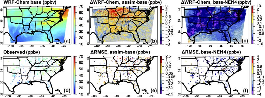
11020                                            M. Huang et al.: Soil moisture, weather, and ozone in the southeastern US

3.2     Soil moisture, weather states, and energy fluxes          ally, the WRF-Chem predicted mean rainfall rates over low-
        during ACT-America                                        precipitation regions (e.g., several Atlantic states) are higher
                                                                  than those based on the Stage IV and GPM rainfall products,
Land and surface weather states as well as energy fluxes from     which tend to overestimate precipitation at the low end (e.g.,
the WRF-Chem base simulation, together with the SMAP              Nelson et al., 2016; Tan et al., 2016). Such positive model
DA impacts on these variables, are illustrated in Fig. 2 (for     biases for low-precipitation regions have also been reported
SM), Figs. 3–4 (for T2, RH, WS, and PBL height, PBLH),            in Barth et al. (2012).
Fig. 5 (for precipitation), and Figs. 6, S3, and S4 (for energy
fluxes and their partitioning) for the 16–28 August 2016 pe-      3.2.2   SMAP DA impacts on SM, surface weather states
riod.                                                                     and energy fluxes

3.2.1    Observed and modeled SM and weather                      Surface SM at the model initial times (i.e., 00:00 UTC each
         conditions                                               day) was broadly reduced by the SMAP DA, except parts
                                                                  of coastal Texas, Ohio, and Florida (Fig. 2d). Such changes
The highest daytime (13:00–24:00 UTC, local time +5 or            in the modeled SM fields are consistent with the modeled
+6) average T2 was observed in several states in the Atlantic     daytime specific humidity (not shown in figures) and RH re-
region that were undergoing drought conditions (Figs. S2,         sponses (Fig. 3m). They are anti-correlated with the model
left; 3b). The daily T2 maxima occurred during noon–early         responses in the averaged daytime T2 and PBLH fields
afternoon in most places, consistent with the findings from       (Fig. 3e; h) as well as their daily amplitudes (not shown in
Huang et al. (2016). The Lower Mississippi River regions          figures). The daytime T2 and RH responses to the SMAP DA
were influenced by high humidity (Fig. 3j). Under the in-         are statistically significant in ∼ 21 % and ∼ 65 % of the over-
fluence of the Bermuda High, surface winds were over-             land model grids, respectively (i.e., p < 0.05 based on Stu-
all mild to the east of Texas. Strongest rainfall affected        dent’s t tests; Fig. 4a–b), with the most significant daytime-
Texas, Arkansas, Kentucky, Tennessee, and near the bor-           averaged responses of ∼ 2 K and > 10 %, respectively, oc-
der of Kansas and Missouri (Fig. 5a–b), which belonged            curring in Missouri and Ohio, as well as several other states
to the wetter-than-normal regions according to August 2016        located within 33–40◦ N and 90–100◦ W. In places, the daily
drought indexes. Rainfall in most areas peaked in the late af-    maxima of WRF-Chem T2 were delayed by an hour or two
ternoon or evening after the times of peak T2 (Fig. 5e–f). The    when the SMAP DA was enabled (Fig. 3g). The changes
observed diurnal cycles of rainfall and T2 indicate that, for     in WRF-Chem temperature gradients due to the SMAP DA
the study area/period, convection was mainly due to the ther-     led to slight WS enhancements over many of the model
modynamic response to surface temperature. However, land–         grids (Fig. 3o). In contrast to the WRF-Chem T2 and RH
sea interactions, fronts, and topography, as well as aerosol      responses, these WS changes are statistically insignificant
loadings may also have come into play.                            (i.e., p > 0.05 based on Student’s t tests) in ∼ 97 % of the
   The dry and wet anomalies in the southeastern US based         overland model grids (Fig. 4c). On the 13 d timescale, the
on the modeled SM (Fig. 2a) are shown to be consistent            SMAP DA had less discernable impacts on rainfall, consis-
with ground-based SM measurements (e.g., Fig. 2c), as well        tent with the findings from Koster et al. (2010, 2011) and
as weekly (not shown in figures) and monthly drought in-          Huang et al. (2018). The SMAP DA impacts on mean rain-
dexes (e.g., Fig. S2, left). The modeled SM values in var-        fall rate and diurnal cycles show noisy patterns (Fig. 5d; g;
ious soil layers are near the model-based soil wilting points     h), and positive and negative SM–precipitation relationships
and field capacities (Fig. S1, middle and lower) over drought-    are both found. The spatial and temporal variability in these
influenced and wetter-than-normal regions, respectively. The      model sensitivities reflects the impacts of local hydrological
WRF-Chem base simulation overall captured the observed            regimes and their anomalies, as well as moisture advection.
patterns of T2, RH, and WS across the domain, with its day-          It is indicated by Fig. 2b and e that, during the study pe-
time PBLH spatially correlated with the T2 patterns (Table 2      riod, the SMAP DA successfully reduced the discrepancies
and Figs. 3a–b; d; i–j; k–l). Referring to the Stage IV and       between SMAP and Noah-calculated surface SM across the
GPM rainfall data, the WRF-Chem base case also repro-             model domain. The modeled surface SM was also cross-
duced the diurnal cycles of rainfall during the study period      validated with ground-based SM measurements at dozens
fairly well overall, but the rainfall hotspots simulated by the   of SCAN sites, using the root-mean-square error (RMSE)
model appear west to those in the Stage IV and GPM prod-          metric. Figure 2f–g show the results based on a compari-
ucts (Fig. 5c). Dirmeyer et al. (2012) found that models’ rain-   son of the modeled surface SM with ∼ 10 cm belowground
fall performance more strongly depended on the distinctive        SM measurements at these SCAN sites. This evaluation sug-
treatment of the model physics than on the model resolu-          gests that the Noah-based SM was more evidently improved
tion. Our WRF-Chem performance for rainfall diurnal cy-           by the SMAP DA at sparsely vegetated regions; i.e., RMSE
cle in this region is similar to previous convection-permitting   was reduced at almost all sites where green vegetation frac-
WRF-Chem simulations (e.g., Barth et al., 2012). Addition-        tion ≤ 0.6. At dense-vegetation (i.e., green vegetation frac-

Atmos. Chem. Phys., 21, 11013–11040, 2021                                         https://doi.org/10.5194/acp-21-11013-2021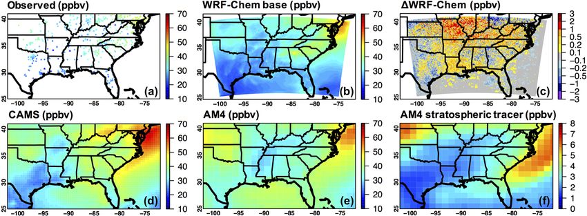
M. Huang et al.: Soil moisture, weather, and ozone in the southeastern US                                                               11021

Figure 2. Period-mean (16–28 August 2016) (a) WRF-Chem base case surface-layer (i.e., 0–10 cm belowground) soil moisture at initial
times and (d) its changes due to the SMAP DA. Panels (b, e) indicate the SMAP DA impacts on the discrepancies between SMAP and
modeled surface soil moisture. Panel (c) presents soil moisture measurements at various SCAN sites at ∼ 10 cm belowground at WRF-Chem
initial times. The SMAP DA impacts on RMSEs of the modeled surface soil moisture, as well as their relationships with the model-based
green vegetation fraction, are shown in (f, g). In (g), the SCAN sites located in cropland areas according to the model’s land use–cover input
are highlighted in red.

Figure 3. Period-mean (16–28 August 2016) WRF-Chem base case daytime (a) 2 m air temperature (T ); (d) PBLH; (i) 2 m relative humidity
(RH); and (k) 10 m wind speed, as well as (e, h, m, o) the impacts of SMAP DA on these model fields. Observed daytime surface T , RH,
and wind speed, as well as the impacts of the SMAP DA on RMSEs of these model fields are shown in (b, f), (j, n), and (l, p) respectively.
Significance test results are included in Fig. 4. The time of daily peak air T in US central standard time (CST), as well as its response to the
SMAP DA, is shown in (c, g).

https://doi.org/10.5194/acp-21-11013-2021                                                 Atmos. Chem. Phys., 21, 11013–11040, 2021
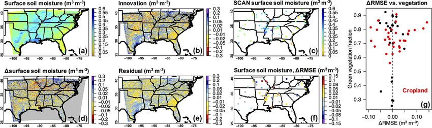
11022                                               M. Huang et al.: Soil moisture, weather, and ozone in the southeastern US

Figure 4. The p values of Student’s t tests comparing the daytime (a) 2 m air temperature (T ); (b) 2 m relative humidity (RH); and (c) 10 m
wind speed from the base and assim cases, plotted against the absolute changes in these model fields due to the SMAP DA. Results are only
presented for the overland model grids.

Figure 5. Period-mean (16–28 August 2016) (a–d) rainfall rate and (e–h) time of peak rainfall in US central standard time (CST) from
(a, e) the National Stage IV Quantitative Precipitation Estimates product; (b, f) the Global Precipitation Measurement; and (c, g) the WRF-
Chem base case. The impacts of the SMAP DA on WRF-Chem results are indicated in (d, g, h).

tion > 0.6) SCAN sites, over a half of which are located in             tations of terrain height can pose challenges for evaluating
cropland areas subject to the impacts of irrigation and other           the modeled surface weather fields with ground-based obser-
human activities, the SMAP DA did not prevalently decrease              vations. The 12 km model grid used in this work represents
or increase the discrepancies between the modeled and mea-              terrain height well (i.e., |model–actual| < 15 m) at over 70 %
sured SM. Similar findings were reached based on such a                 of the model grids that have collocated observations, but at
comparison of the modeled surface SM and ∼ 5 cm below-                  some locations the discrepancies between the model and ac-
ground SM measurements at these SCAN sites. The over-                   tual terrain height exceed 100 m. Furthermore, human activ-
all T2, RH, and WS performance of WRF-Chem was not                      ities such as irrigation can significantly modify water budget
prevalently improved or degraded due to the inclusion of the            and land–atmosphere coupling strength over agricultural re-
SMAP DA (e.g., Fig. 3f; n; p, based on the RMSE metric);                gions (e.g., Lu et al., 2017), but these processes were unac-
i.e., improvements on T2, RH, and WS occurred in 47 %,                  counted for in the modeling system used. Observations from
51 %, and 52 % of the model grids where observations are                SMAP and other satellites are capable of detecting the sig-
available, and the domain-wide mean RMSE changes for T2,                nals of irrigation over the southeastern US (e.g., the circled
RH, and WS are ∼ 0 K, −0.024 %, and −0.005 m s−1 , re-                  regions in Fig. 1c based on Ozdogan and Gutman, 2008, and
spectively (Table 2). This finding for dense vegetation re-             Zaussinger et al., 2019) and other regions of the world. How-
gions is qualitatively consistent with the findings in Huang            ever, for locations where irrigation or/and other missing pro-
et al. (2018) and Yin and Zhan (2018), which are based                  cesses dominantly contributed to the systematic biases be-
on RMSE and other evaluation metrics, and it may par-                   tween the modeled and SMAP SM, the bias correction ap-
tially be attributed to SMAP retrieval quality and the land–            proach applied may have removed the information of these
atmosphere feedbacks represented in Noah. Additionally, as              processes from the SMAP observations before the DA. As a
discussed in Huang et al. (2018), unrealistic model represen-           result, the DA may not be effective at these locations. How

Atmos. Chem. Phys., 21, 11013–11040, 2021                                                 https://doi.org/10.5194/acp-21-11013-2021
M. Huang et al.: Soil moisture, weather, and ozone in the southeastern US                                                                                           11023

Figure 6. Period-mean (16–28 August 2016) daily evaporative fraction, defined as daily latent heat / (daily latent heat + daily sensible heat),
from (a) a FLUXCOM product; (b) selected FLUXNET sites; and (c) the WRF-Chem base case. Panel (d) shows the impact of the SMAP
DA on WRF-Chem evaporative fraction. Additional evaluation results for latent and sensible heat fluxes at the focused FLUXNET sites are
presented in Fig. S3.

Table 2. The SMAP DA impacts on modeled surface meteorological and O3 fields, as well as their agreement with observations.

  Variable analyzed                      Assim–base case,            RMSE, base case,                 1RMSE,                           Percentage of the model grids
                                         domain mean ±               domain mean ±                    Assim–base case,                 with available observations
                                         standard deviation,         standard deviation               domain mean ±                    in which the SMAP data
                                         for all overland grids                                       standard deviation               assimilation improved
                                                                                                                                       the model performance
  Daytime 2 m air temperature            0.099 ± 0.373 K             2.177 ± 0.718 K                  ∼ 0 ± 0.165 K                    47.2 %
  Daytime 2 m relative humidity          −0.573 ± 3.225 %            12.633 ± 4.188 %                 −0.024 ± 1.765 %                 51.3 %
  Daytime 10 m wind speed                0.001 ± 0.129 m s−1         1.714 ± 0.831 m s−1              −0.005 ± 0.183 m s−1             52.5 %
  MDA8 O3                                0.141 ± 0.494 ppbv          7.674 ± 2.473 ppbv               0.057 ± 0.372 ppbv               42.0 %
                                                                     (referring to AQS);              (referring to AQS);              (referring to AQS);
                                                                     6.710 ± 2.285 ppbv               0.007 ± 0.343 ppbv               51.4 %
                                                                     (referring to CASTNET)           (referring to CASTNET)           (referring
                                                                                                                                       to CASTNET)

 Acronyms: AQS: Air Quality System; CASTNET: Clean Air Status and Trends Network; MDA8: daily maximum 8 h average; RMSE: root-mean-square error; SMAP: Soil Moisture Active
 Passive.

irrigation patterns and scheduling, depending in part on the                             and RH, with the maxima (> 0.75) seen in the Lower Mis-
weather conditions, affected our WRF-Chem performance,                                   sissippi River region and smaller values (< 0.65) in the dry
as well as the effectiveness of the SMAP bias correction and                             Atlantic states and some parts of the Southern Great Plains
DA, is worth further investigations. In places, the changes in                           (Fig. 6a–b). Note that the absolute latent and sensible heat
WRF-Chem rainfall patterns due to the SMAP DA are within                                 fluxes can differ significantly at locations with similar evapo-
the discrepancies between the Stage IV and GPM rainfall                                  rative fraction values (Fig. S3). The WRF-Chem-based evap-
products. A better understanding of the uncertainty associ-                              orative fraction shows similar spatial gradients but is over-
ated with these two rainfall products used can benefit the                               all negatively biased (Fig. 6c). The changes in WRF-Chem
assessment of SM DA impacts on the model’s precipitation                                 evaporative fraction due to the SMAP DA are spatially cor-
performance.                                                                             related with the surface moisture changes (Figs. 2d; 3m; 6d).
   The spatial patterns of evaporative fraction (defined as la-                          As a result, the model performance of evaporative fraction
tent heat / (latent heat + sensible heat)) follow those of SM                            was only improved over some of the regions where it was

https://doi.org/10.5194/acp-21-11013-2021                                                                    Atmos. Chem. Phys., 21, 11013–11040, 2021
11024 M. Huang et al.: Soil moisture, weather, and ozone in the southeastern US
increased by the SMAP DA. It is found that the SMAP DA 3.3 Ozone and its responses to the SMAP DA during
impacts on model performance are not universally consistent ACT-America
for surface energy fluxes and land–atmosphere states. This
can be explained by the fact that the modeling system used 3.3.1 Surface O3
has shortcomings in representing SM–flux coupling and/or
the relationships between moisture and heat fluxes and the The changes in the above-discussed meteorological vari-
atmospheric weather which need to be clearly identified and ables (e.g., air temperature, humidity, WS, PBLH) due to
corrected. The most possible reasons causing such model be- the SMAP DA alter various atmospheric processes which
haviors include the following: (1) irrigation and other pro- can have mixed impacts on surface O3 concentrations. For
cesses related to human activities were unaccounted for, and example, warmer environments promote biogenic VOC and
the surface exchange coefficient CH , which is a critical pa- soil NO emissions as well as accelerating chemical reactions
rameter controlling energy transport from the land surface to (e.g., many oxidation processes, thermal decomposition of
the atmosphere, may not be realistically represented in Noah peroxyacetyl nitrate). These will be discussed in detail in
(details in Sect. S1); (2) the SMAP DA did not update the the following paragraphs referring to Figs. 9 and S5. Faster
vegetation and surface albedo fields in Noah, which was un- winds and thickened PBL dilute air pollutants including O3
realistic; and (3) soil parameters determined from soil tex- and its precursors and therefore reduce O3 destruction via
ture types and a lookup table may be inaccurate in places. titration (i.e., O3 + NO → O2 + NO2 ) as well as photochem-
To confirm and address these limitations in the modeling/DA ical production of O3 . The changes in wind vectors affect
system used, and to identify other possible reasons, future pollutants’ concentrations in downwind regions. Water va-
efforts should be devoted to applications using other LSMs por mixing ratios perturb O3 photochemical production and
(e.g., the Noah-Multiparameterization) and up-to-date inputs loss via affecting the HOx cycle. Their impacts on O3 levels
and parameters (e.g., soil texture types and lookup tables), depend on the chemical environments of the areas of interest;
together with multivariate land DA; evaluation of additional i.e., in general, reduced specific humidity slightly enhances
water and energy flux variables such as runoff and radiation, O3 , except in some polluted regions. Also, higher RH is of-
the latter of which shows inconsiderable sensitivities to the ten associated with cloud abundance and solar radiation and
SMAP DA (Fig. S4); and utilization of alternative WRF in- therefore slows down the photochemical processes (Camalier
puts and physics configurations. et al., 2007). Additionally, chemical loss via stomatal uptake
may be slower under lower SM and humidity and higher tem-
3.2.3 SMAP DA impacts on weather conditions at perature conditions, and nonstomatal uptake also varies with
various altitudes meteorology. These processes, however, may not all be re-
alistically represented by the Wesely dry deposition scheme
The WRF-Chem-modeled weather states were also evaluated (Sects. 2.1 and S2; Figs. S1 and S7) used in this study.
with ACT-America aircraft observations at various altitudes. Figure 10a–b compare the observed and WRF-Chem base
Along the flight paths, the observed air temperature and wa- case daytime surface O3 during 16–28 August 2016, and
ter vapor mixing ratios decrease with altitude, which were the SMAP DA impacts on daytime surface O3 are shown
captured by WRF-Chem fairly well (Figs. 7a–b; e–f and 8a; in Fig. 10c. Low-to-moderate O3 pollution levels are seen
c). The modeled air temperature and humidity as well as over most areas within the model domain, except the At-
their responses to the SMAP DA vary in space and time. lantic states due to the influences of frequent air stagnation
In general, these responses are particularly strong near the and warm and dry conditions. Period-mean daytime surface
surface, where the majority of the samples were collected. O3 responses to the SMAP DA are overall slightly positive
Under stormy weather conditions on 16, 20, and 21 August but exceed or closely approach 2 ppbv in some places in Mis-
2016, the maximum changes in air temperature and humid- souri, Illinois, and Indiana, and the strongest decreases in the
ity in the free troposphere exceed 2.3 K and 2 g kg−1 , re- period-mean daytime surface O3 occurred in Ohio (i.e., by
spectively (Fig. 7c; g). Corresponding to these changes, the > 2 ppbv). The averaged O3 changes show strong spatial cor-
SMAP DA modified the RMSEs of WRF-Chem air temper- relations (with correlation coefficient r values of ∼ 0.8) with
ature and/or water vapor by over 5 % for several individ- those of T2 and PBLH (Fig. 3e; h), which are anti-correlated
ual flights and reduced the RMSEs of these model variables with the surface humidity responses (Figs. 2d and 3m). On
overall by ∼ 0.7 % and ∼ 2.3 %, respectively (Fig. 8b). The most of the days during 16–28 August 2016, the maximum
most significant improvements in the modeled weather states impacts of SMAP DA on daily daytime surface O3 exceed
occurred at ≥ 800 hPa, where the maximum improvements in 4 ppbv, and the O3 sensitivities are moderately correlated
air temperature and water vapor exceed 2.6 K and 2 g kg−1 , with the daytime T2 changes (Fig. 11a, with r values within
respectively, and their RMSEs were both reduced by ∼ 2.7 % 0.4–0.7). The period-mean WRF-Chem surface MDA8 and
(Figs. 7d; h and 8d). its response to the SMAP DA (Fig. 12a–b) show similar spa-
tial patterns to those of the modeled surface daytime O3 but
are of higher variability.
Atmos. Chem. Phys., 21, 11013–11040, 2021 https://doi.org/10.5194/acp-21-11013-2021You can also read