SURVEY OF DATA ASSIMILATION METHODS FOR CONVECTIVE-SCALE NUMERICAL WEATHER PREDICTION AT OPERATIONAL CENTRES - DIVA
←
→
Page content transcription
If your browser does not render page correctly, please read the page content below
Quarterly Journal of the Royal Meteorological Society                                                   Q. J. R. Meteorol. Soc. (2018) DOI:10.1002/qj.3179

  Survey of data assimilation methods for convective-scale numerical
               weather prediction at operational centres
   Nils Gustafsson,a * Tijana Janjić,b Christoph Schraff,c Daniel Leuenberger,d Martin Weissmann,e
    Hendrik Reich,e Pierre Brousseau,f Thibaut Montmerle,f Eric Wattrelot,f Antonı́n Bučánek,g
Máté Mile,h Rafiq Hamdi,i Magnus Lindskog,a Jan Barkmeijer,j Mats Dahlbom,k Bruce Macpherson,l
  Sue Ballard,l Gordon Inverarity,l Jacob Carley,n Curtis Alexander,m David Dowell,m Shun Liu,n
                                 Yasutaka Ikutao and Tadashi Fujitao
                                        a
                                   Swedish Meteorological and Hydrological Institute, Norrköping, Sweden
                               b Hans
                                  Ertel Centre for Weather Research, Deutscher Wetterdienst, München, Germany
                                                 c Deutscher Wetterdienst, Offenbach, Germany
                             d
                               Federal Office of Meteorology and Climatology, MeteoSwiss, Zürich, Switzerland
                     e
                       Hans Ertel Centre for Weather Research, Ludwig-Maximilians-Universität München, Germany
                        f
                          Centre National de Recherches Météorologiques (Météo-France/CNRS), Toulouse, France
                                         g Czech Hydrometeorological Institute, Praha, Czech Republic
                                             h
                                               Hungarian Meteorological Service, Budapest, Hungary
                                         i
                                           Royal Meteorological Institute of Belgium, Brussels, Belgium
                                     j
                                       Royal Meteorological Institute of Netherlands, De Bilt, Netherlands
                                            k
                                              Danish Meteorological Institute, Copenhagen, Denmark
                                                             l Met Office, Exeter, UK
                                                        m
                                                          NOAA/ESRL, Boulder, CO, USA
                                   n
                                     NOAA/NCEP/EMC and IM Systems Group, College Park, MD, USA
                                                   o
                                                     Japan Meteorological Agency, Tokyo, Japan
    *Correspondence to: N. Gustafsson, SMHI, Folkborgsvägen 17, 60176 Norrköping, Sweden. E-mail: nils.gustafsson@smhi.se
          This article is published with the permission of the Controller of HMSO and the Queen’s Printer for Scotland.

                Data assimilation (DA) methods for convective-scale numerical weather prediction at
                operational centres are surveyed. The operational methods include variational methods
                (3D-Var and 4D-Var), ensemble methods (LETKF) and hybrids between variational
                and ensemble methods (3DEnVar and 4DEnVar). At several operational centres, other
                assimilation algorithms, like latent heat nudging, are additionally applied to improve
                the model initial state, with emphasis on convective scales. It is demonstrated that
                the quality of forecasts based on initial data from convective-scale DA is significantly
                better than the quality of forecasts from simple downscaling of larger-scale initial data.
                However, the duration of positive impact depends on the weather situation, the size of
                the computational domain and the data that are assimilated. Furthermore it is shown that
                more advanced methods applied at convective scales provide improvements over simpler
                methods. This motivates continued research and development in convective-scale DA.
                   Challenges in research and development for improvements of convective-scale DA are
                also reviewed and discussed. The difficulty of handling the wide range of spatial and temporal
                scales makes development of multi-scale assimilation methods and space–time covariance
                localization techniques important. Improved utilization of observations is also important. In
                order to extract more information from existing observing systems of convective-scale phe-
                nomena (e.g. weather radar data and satellite image data), it is necessary to provide improved
                statistical descriptions of the observation errors associated with these observations.
                Key Words:     data assimilation; numerical weather prediction; convective-scale
                Received 31 March 2017; Revised 6 October 2017; Accepted 9 October 2017; Published online in Wiley Online Library

[The copyright line for this article was changed on 18 July 2018 after original publication]

c 2018 The Authors and Crown Copyright, Met Office. Quarterly Journal of the Royal Meteorological Society published by John Wiley & Sons Ltd on behalf of the
Royal Meteorological Society.
This is an open access article under the terms of the Creative Commons Attribution License, which permits use, distribution and reproduction in any medium,
provided the original work is properly cited.
N. Gustafsson et al.

1. Introduction                                                                     Also associated with the spatial scale is the growing importance
                                                                                of nonlinearity, moist physical processes and unbalanced flows
Development of data assimilation (DA) methods for global                        at convective scales (Pagé et al., 2007). With nonlinearity comes
numerical weather prediction (NWP) models started with                          flow dependence, since the structures of the convective-scale
simple horizontal interpolation methods (Eliassen, 1954) which                  phenomena are dependent on the actual state of the large-
gradually developed to become three-dimensional and to also                     scale forcing. The moist physical processes, for example latent
include multivariate relationships (Lorenc, 1981). Variational                  heating, trigger unbalanced adjustment processes. This means that
methods were introduced to utilize the model dynamics in the DA                 adjustment processes and associated unbalanced flow structures
process (Le Dimet and Talagrand, 1986) and four-dimensional                     have to be taken into account during the DA. The tools
variational DA is now applied operationally (Rabier et al., 2000).              which we have developed for synoptic-scale DA, for example
In order to take into account flow-dependence of forecast errors                linear balances and static background-error constraints, are no
in the DA process, various forms of Ensemble Kalman Filters                     longer appropriate. Steps that have been taken to introduce
(EnKF; Evensen, 1994) have become competitive with variational                  flow dependence in synoptic-scale DA will certainly be even
techniques for atmospheric DA. More recently, hybrids between                   more important for convective-scale DA. It is an open question,
variational and ensemble DA techniques have been proposed                       however, to what extent these techniques will be completely
(Lorenc, 2003; Liu et al., 2008) and are becoming mainstream in                 satisfactory for convective-scale DA, or whether fully nonlinear
DA for global NWP at operational centres (review by Bannister,                  DA techniques like particle filters (van Leeuwen, 2009) will be
2017).                                                                          required, or if modifications to hybrid and ensemble methods to
    The DA problem for convective-scale NWP differs from the                    deal with non-Gaussianity, as suggested in Janjić et al. (2014),
global problem in several respects. The higher model resolution                 Hodyss (2011) and Bishop (2016), would be sufficient.
demands dense observations at a suitable temporal and spatial                       This manuscript provides a survey of DA methods for
resolution. Given that convective systems are often a primary                   convective-scale NWP. As atmospheric DA for convective scales
forecast aspect, these observations should ideally be related                   is in a quite early stage of development, the reader may notice that
to convection: either of their environmental conditions or of                   we do not all fully agree on fundamental principles for convective-
the convective systems themselves. There is a wide variety of                   scale DA – questions related to spatial scales and imbalance, for
                                                                                example. By making these questions and disagreements visible
observations available that are not yet exploited in regional DA
                                                                                through this article, we will be able to take further steps to a joint
systems:
                                                                                understanding as a starting point for further developments.
(i) only a very small fraction of available satellite observations is
                                                                                    Section 2 of this article describes operational DA methods
currently used, in particular for cloud-affected observations;
                                                                                for convective scales and section 3 discusses the impact of
(ii) the costs of many ground-based remote-sensing instruments
                                                                                these methods for operational NWP. Challenges in research
have reduced significantly, which allows the installation of new
                                                                                for development of convective-scale DA methods are discussed
sensor networks, and
                                                                                in section 4 and a summary and some concluding remarks
(iii) useful information could be extracted from various
                                                                                are provided in section 5. A list of acronyms used is provided in
observations made for other purposes (e.g. car or mobile phone
                                                                                Table 1 and a glossary of observations and intruments is contained
sensors, output of wind and solar power production, visibility                  in Table 2. In general, only the acronym will be used in the text.
sensors, etc.).
However, little knowledge exists on where the community should
                                                                                2. Description of operational methods
put its emphasis regarding the refinement of observational
networks and the development of suitable observation operators
and assimilation methods. A few recent studies have exploited                   Data assimilation systems for convective-scale NWP are presented
ensemble information to estimate the contribution of various                    and discussed here for the following organizations:
observations to the reduction of analysis error (Brousseau                          1. Météo-France, the national weather service of France.
et al., 2014) or forecast sensitivity to observations (Sommer                       2. The ALADIN and RC LACE consortia with participation of
and Weissmann, 2016).                                                                  the weather services of Algeria, Austria, Belgium, Bulgaria,
    One may ask which atmospheric variables would be most                              Czech Republic, Croatia, France, Hungary, Morocco,
efficient for assimilation at convective scales. Considering the                       Poland, Portugal, Romania, Slovakia, Slovenia, Turkey
geostrophic adjustment process, we may hypothesize that wind                           and Tunisia.
field information becomes relatively more important than mass                       3. The HIRLAM consortium with participation of the weather
field information. Simulation and sensitivity experiments with                         services of Denmark, Estonia, Finland, France, Iceland,
convective-scale models may provide us with more details on the                        Ireland, Latvia, Lithuania, the Netherlands, Norway, Spain
relative importance of different meteorological variables as initial                   and Sweden.
conditions. Fabry and Sun (2010) investigated the sensitivity                       4. The Met Office, the national weather service of the UK.
of the Weather Research and Forecasting (WRF) model to                              5. The COSMO consortium with participation of the weather
spatially coherent perturbations of different model variables for                      services of Germany, Italy and Switzerland.
initialization of convective storms. They concluded that the state                  6. NOAA, the National Oceanic and Atmospheric Adminis-
of the model atmosphere after a few hours of model integration,                        tration of the USA.
measured through an energy norm, was mostly sensitive to the                        7. JMA, the Japan Meteorological Agency.
initial vertical profiles of moisture, wind and temperature in the
lower and middle troposphere. Vertical profiles of cloud and                      An overview of the operational DA and forecasting systems of
precipitation particles were of less importance, partly due to their            these organizations is provided in Tables 3–6. Table 3 describes
lower predictability.                                                           the forecast models, Table 4 the core assimilation methods, Table 5
    The question of spatial scale is of crucial importance for DA.              the operational cycling of DA at the different centres and Table 6
For convective-scale DA we may need to know both the synoptic                   the observing systems used.
scales forcing the mesoscale phenomena and also information
on the convective scales that we want to predict. A complicating                2.1.   Formulation of the different DA methods
factor is the difficulty of recovering all the scales resolved over a
regional model domain using only observations from inside the                   In order to describe and discuss the assimilation techniques,
domain. As will be discussed here, there are many open questions                we will here provide a brief description of their mathematical
and many suggested solutions with regard to the handling of                     formulations. The notations follow Lorenc (2013) and Bannister
synoptic and meso scales in convective-scale DA.                                (2017).

   c 2018 The Authors and Crown Copyright, Met Office. Quarterly Journal of the                   Q. J. R. Meteorol. Soc. (2018)
Royal Meteorological Society published by John Wiley & Sons Ltd on behalf of the Royal Meteorological Society.
Data Assimilation Methods for Convective-scale NWP
Table 1. List of acronyms. Table 1. Continued
Acronym Description QC Quality Control
RAP RApid Refresh mesoscale analysis and prediction system
3D-Var Three-dimensional Variational DA
RC LACE Regional Cooperation for Limited-Area modelling in Central
3DEnVar Three-dimensional Ensemble Variational DA
Europe
4D-Var Four-dimensional Variational DA
RGB Red, Green, Blue colour table
4DEnVar Four-dimensional Ensemble Variational DA
RMSE Root Mean Square Error
AD ADjoint
RRTMG Rapid Radiative Transfer Model for General circulation model
AEARP Assimilation d´Ensemble ARPege
applications
ALADIN Aire Limitée Adaptation dynamique Développement InterNa-
RTPP Relaxation-To-Prior Perturbations
tional
RUC Rapid Update Cycle/ing
– Limited-Area Model (LAM) and LAM consortium
SPPT Stochastic Perturbations of Physical Tendencies
ALARO Physical parametrization package for ALADIN
SURFEX SURFace EXternalisée – a surface parametrization package
AROME Applications de la Recherche l´Opérationnel à Méso-Echelle
TERRA COSMO surface parametrization scheme
– Convective-scale Limited-Area Model
TKE Turbulent Kinetic Energy
ARPEGE Action de Recherche Petite Echelle Grande Echelle – Global
TL Tangent Linear
Model
UKV The UK Variable-resolution model (Met Office)
ASUCA JMA high-resolution model
VarBC Variational Bias Correction
BSS Brier Scill Score
VWC Volume Water Content
CONUS-NAM CONtiguous United States nest of North American Mesoscale
WoF Warn-on-Forecast – NOAA development project
system
WMO World Meteorological Organization
– convective-scale forecasting system
WRF Weather Research and Forecasting model
COSMO COnsortium for Small scale MOdeling
CRPS Continuous Ranked Probability Score
DA Data Assimilation
DF Digital Filter 2.1.1. Incremental 3D-Var and incremental 4D-Var
DFI DF Initialization
DPCG Double Preconditioned Conjugate Gradient
DWD Deutscher WetterDienst
Let x denote the model state of dimension n. The following cost
ECMWF European Centre for Medium-range Weather Forecasts function J is minimized with respect to the assimilation increment
EDA Ensemble Data Assimilation δx = x − xb in incremental 4D-Var:
EKF Extended Kalman Filter
1 T −1
EnKF Ensemble Kalman Filter J = Jb + Jo = δx B δx
EOF Empirical Orthogonal Functions 2
1
EPS Ensemble Prediction System K
ERA ECMWF Re-Analysis projects + (Hk Mk δx−dk )T Rk−1(Hk Mk δx−dk ), (1)
ETKF Ensemble Transform Kalman Filter 2
k=0
EUMETNET EUropean METeorological services NETwork
FGAT First Guess at Appropriate Time where xb is the model background state valid at time t0 , B is the
FSS Fractions Skill Score
GFS Global Forecasting System, the global model of NCEP
background-error covariance matrix and the subscript k denotes
GSM Global Spectral Model at JMA time tk = t0 + kT within the assimilation window from time t0
HARMONIE HIRLAM ALADIN Research on Mesoscale Operational NWP to time tK for regular time interval T, dk = yk − Hk (Mk (xb ))
In Europe are the innovations, with yk being the vector of observations at
– convective-scale forecasting system time tk , Mk (·) denotes integration of the nonlinear model from
HE-VI Horizontally Explicit Vertically Implicit time-stepping time t0 until time tk and Mk denotes the corresponding TL model
HIRLAM HIgh-Resolution Limited-Area Modelling – LAM model and integration, linearized around the background trajectory Mk (xb ).
LAM consortium Rk is the observation-error covariance matrix, Hk (·) is the nonlin-
HRRR High-Resolution Rapid Refresh system – convective-scale
forecasting system
ear observation operator, and Hk is the corresponding TL obser-
IAU Incremental Analysis Update vation operator, linearized around Mk (xb ), all valid at time tk .
ICON ICOsahedral Non-hydrostatic (atmospheric model) In the basic 3D-Var and 4D-Var formulations used in
IFS Integrated Forecast System operations at convective scales, the covariance matrix B is static
IPW Integrated Precipitable Water and not dependent on the forecast errors ‘of the day’. Due to
JAXA Japan Aerospace eXploration Agency its large dimension, the inverse B−1 cannot be obtained directly
JMA Japan Meteorological Agency by matrix inversion techniques. Therefore we introduce a pre-
JMA-NHM JMA Non-Hydrostatic Model conditioning matrix U such that B = UUT , δx = Uχ and χ is
JNoVA JMA Non-hydrostatic model-based Variational DA system
KENDA Kilometre-scale ENsemble DA
the assimilation control variable. With this choice J b = χ T χ /2.
LA Local Analysis – JMA convective-scale DA system The transformation matrix U may be given as a series of simpler
LAM Limited Area Model transform operators that define the background-error covariance
LBC Lateral Boundary Condition model. The order in which these operators are carried out
LETKF Local Ensemble Transform Kalman Filter is important (Bannister, 2008). In the HARMONIE-AROME
LFM Local Forecast Model – JMA convective-scale forecast model formulation (see below), balance operator transforms are carried
LHN Latent Heat Nudging out in spectral space, which makes these balance operators scale-
MA Mesoscale Analysis – JMA mesoscale assimilation system dependent. Compared to what is usually done at global scales,
MSM MesoScale Model – JMA mesoscale model
MY2.5 Mellor–Yamada 2.5 turbulence parametrization
an additional multivariate relationship may be used for specific
MYJ Mellor–Yamada–Janjić planetary boundary-layer scheme humidity following Berre (2000), which is of great interest at
NAM North American Mesoscale system convective scales where the coupling between humidity and
NDP Nowcasting Demonstration Project divergence, for example, can be important.
NCEP National Centers for Environmental Prediction The minimization of the cost function J is done iteratively by
NICT National Institute of Information and Communications calculation of the gradient ∇χ J with respect to the control vector χ
Technology (Japan) and application of, for example, conjugate gradient minimization.
NMC National Meteorological Center (USA) The spatial resolution of the assimilation increment can be
NOAA National Oceanic and Atmospheric Administration (USA)
NWP Numerical Weather Prediction
reduced, making 4D-Var computationally more tractable.
OI Optimal Interpolation Standard incremental 3D-Var is obtained from Eq. (1) by
referring all observations to the start of the assimilation window
c 2018 The Authors and Crown Copyright, Met Office. Quarterly Journal of the Q. J. R. Meteorol. Soc. (2018)
Royal Meteorological Society published by John Wiley & Sons Ltd on behalf of the Royal Meteorological Society.
N. Gustafsson et al.

              Table 2. Glossary of observations and instruments.                  t0 and 3D-Var FGAT by making the TL model an identity operator
                                                                                  Mk = I and, preferably, referring the assimilation increment to
Name             Description                                                      the middle of the assimilation window.
ACARS            Aircraft Communications Addressing and Reporting System
AIREP            AIRcraft REPorts                                                 2.1.2.    Multi-incremental 4D-Var
AIRS             Atmospheric InfraRed Sounder (satellite instrument)
AMDAR            Aircraft Meteorological DAta Relay
AMeDAS           Automated Meteorological Data Acquisition System
                                                                                  The nonlinearities of the forecast model and the observation
AMSR             Advanced Microwave Scanning Radiometer (satellite instru-        operators may be better treated by iterative relinearizations
                 ment)                                                            in an outer loop by splitting the minimization into a series
AMSU             Advanced Microwave Sounding Unit (satellite instrument)          (τ = 1, . . . , Nτ ) of quadratic sub-problems to determine δxτ ,
                                                                                                                     τ
AMV              Atmospheric Motion Vector                                        with the total increment δx= N             τ
                                                                                                                      τ =1 δx . The cost-function for
Aqua             Multi-national scientific research satellite                     each subproblem τ is given by (Courtier et al., 1994)
ARAMIS           Application Radar Á la Météorologie Infra-Synoptique
ASCAT            Advanced SCATterometer (satellite instrument)                             Jτ =Jτb + Jτo
ATMS             Advanced Technology Microwave Sounder (satellite instru-
                                                                                               1
                 ment)
                                                                                              = {δxτ − (xb − xτ )}T B−1 {δxτ − (xb − xτ )}
ATOVS            Advanced TIROS Operational Vertical Sounder (system of                        2
                 sounding instruments on NOAA TIROS series of satellites)
                                                                                                   1 τ τ τ
                                                                                                      K
BALTRAD          BALTex RADar (Radar network in the Baltic Sea area)                            +        (Hk Mk δx −dτk )T Rk−1 (Hτk Mτk δxτ −dτk ),   (2)
BUFR             Binary Universal Form for the Representation of meteorological                    2
                                                                                                     k=0
                 data
BUOY             Reporting format for buoy measurements                           where dτk = yk − Hk (Mk (xτ )), Mτk is the TL forecast model
CRIS             CRoss-track Infrared Sounder (satellite instrument)
                                                                                  linearized around the guess trajectory Mk (xτ ) and Hτk is the
CSR              Clear-Sky Radiance
DMSP             Defense Meteorological Satellite Program
                                                                                  TL observation operator also linearized around Mk (xτ ). The
DPOL             Dual POLarimetric (radar)                                        initial guess x1 = xb is typically used and, starting from τ = 1,
GCOM             Global Change Observation Mission (JAXA satellite)               Eq. (2) is then minimized to find δxτ , after which the guess
GeoCloud         Cloud fraction profiles based on satellite                       state is updated with xτ +1 = xτ + δxτ . The spatial resolution
                 cloud top information                                            of the increment may differ between different outer-loop
GMI              Global Microwave Imager (satellite instrument)                   iterations.
GNSS             Global Navigation Satellite System
GOES             Geostationary Operational Environmental Satellite
GPM              Global Precipitation Measurement                                 2.1.3.    The hybrid 3DEnVar and the hybrid 4DEnVar
GPM/DPR          Global Precipitation Measurement/Dual-frequency Precipita-
                 tion Radar
                                                                                  The aim of hybrid variational ensemble DA methods is to combine
GPS              Global Positioning System
GPS-RO           GPS Radio Occultation
                                                                                  the robustness and full-rank covariance matrix of variational
HDF5             Hierarchical Data Format                                         methods with the flow-dependence of ensemble methods. For
Himawari         Japan meteorological satellite                                   a simplest possible 3DEnVar, we may follow Liu et al. (2008)
HIRS             High-resolution InfraRed Sounder (satellite instrument)          and replace the static error covariance B in (1) with a flow-
IASI             Infrared Atmospheric Sounding Interferometer (satellite          dependent error covariance P = XXT estimated from an ensemble
                 instrument)                                                      of background model states. X is a matrix whose columns are the
IR               InfraRed                                                         normalized deviations of the ensemble background states from
MDCARS           Meteorological Data Collection And Reporting System
MESONET          MESO-scale surface station NETwork                               their mean xb :
METAR            Format for reporting weather information (aviation)                                 1
METOP            European meteorological polar orbiting satellites                         X= √              xb,1 − xb , . . . , xb,Nens − xb , (3)
MHS              Microwave Humidity Sounder (satellite instrument)                                Nens − 1
Mode-S EHS       Mode-S EnHanced Surveillance winds                               where Nens is the number of ensemble members. We may apply X
                  – winds obtained from air traffic control systems
MRAR             Mode-S Meteorological Routine Air Report
                                                                                  for the pre-conditioning δx = Xχ . The control vector χ will have
MSG              Meteosat Second Generation                                       the dimension of the number of ensemble members and we can
                  – European operational meteorological geostationary satellite   notice that the assimilation increment is just a linear combination
MUAC             Maastricht Upper Air Control                                     of the ensemble perturbations.
MW               MicroWave                                                           Although flow-dependence has been achieved, this simple
NPP              The SUOMI National Polar-orbiting Partnership                    3DEnVar will suffer from two problems. Due to the limited num-
ODIM             OPERA Data Information Model                                     ber of ensemble members (Nens ∼ 10 − 100) small-amplitude
OPERA            Operational Program for the Exchange of weather RAdar            covariances will be poorly represented, resulting in noisy assimi-
                 information
PILOT            Balloon wind profile observations
                                                                                  lation increments. Furthermore, the spatial variations in a small
PIREP            PIlot weather REPort                                             ensemble may not describe all observed structures of importance.
RASS             Radio Acoustic Sounding System                                   Standard remedies to these problems are to introduce covari-
RTTOV            Radiative Transfer for TOVS (software package)                   ance localization and to combine the ensemble covariance with a
SAF              Satellite Application Facility                                   static full-rank covariance (hybridization). Localization in model
SEVIRI           Spinning Enhanced Visible and InfraRed Imager (satellite         space is generally carried out by a Schur product (element-by-
                 instrument)                                                      element multiplication) of the ensemble covariance matrix P
SHIP             Format for marine (ship) observations                            with a localization matrix C, Ploc = C ◦ P, where the elements
SSMIS            Special Sensor Microwave Imager/Sounder (satellite instru-
                                                                                  of the localization matrix force the covariances to become zero
                 ment)
SUOMI            Satellite named after the scientist Verner Suomi                 for grid separations larger than a pre-defined localization length-
SYNOP            Format for SYNOPtic land surface observations                    scale. Lorenc (2003) proposed that the covariance localization
TEMP             Format for radiosonde TEMPerature, humidity and wind             could be carried out through a Schur product between local-
                 profiles                                                         ized weights, included in an augmented control vector, and the
TIROS            Television InfraRed Observation Satellite programme              ensemble background perturbations. The mathematical equiva-
TOVS             TIROS Operational Vertical Sounder                               lence of differently posed hybrid methods was proven by Wang
WPR              Wind Profiling Radar                                             et al. (2007) and a comprehensive review has been published by
ZTD              Zenith Total Delay
                                                                                  Bannister (2017). We will briefly describe the method suggested

   c 2018 The Authors and Crown Copyright, Met Office. Quarterly Journal of the                   Q. J. R. Meteorol. Soc. (2018)
Royal Meteorological Society published by John Wiley & Sons Ltd on behalf of the Royal Meteorological Society.
Table 3. Main characteristics of the AROME-France, HARMONIE-AROME, ALADIN, COSMO, UKV, CONUS NAM, HRRR, MSM and LFM models.
Model/Centre Geometry Physics Dynamics Coupling References
AROME-France/ Spectral, 2D Fourier Non-hydrostatic; Davies relaxation;
Météo-France Linear grid 1.3 km AROME Semi-implicit; ARPEGE synchron. Seity et al. (2011)
90 hybrid levels Semi-Lagrangian
1500 × 1400 points
HARMONIE-AROME/ Spectral, 2D Fourier Adapted Non-hydrostatic; Davies relaxation;
HIRLAM Linear grid 2.5 km AROME Semi-implicit; ECMWF forecasts Bengtsson et al. (2017)
65 hybrid levels Semi-Lagrangian (6 h lag)
ALADIN/ Spectral, 2D Fourier ALARO-1 Hydrostatic or Davies relaxation;
ALADIN Linear grid 2.5 km or AROME non-hydrostatic; ARPEGE synchr. or Szintai et al. (2015)
and RC LACE 90 hybrid levels Semi-implicit; ECMWF (6 h lag)
Semi-Lagrangian;
COSMO/ Arakawa C 1-moment 5-category cloud Non-hydrostatic; ICON ensemble (0 h lag); Baldauf (2010)
DWD and DWD: 2.8 km microphysics; Shallow convection; Time-splitting MeteoSwiss: ECMWF ensemble Baldauf et al. (2011)
MeteoSwiss 50 hybrid levels Prognostic TKE modified MY2.5; (IFS high res. 6 h lag Wicker and Skamarock (2002)
421 × 461 points Radiation of Ritter and Geleyn; ensemble mean, IFS ensemble Raschendorfer (2001)
MeteoSwiss: 2.2 km Surface scheme TERRA 3D extension for perturbations 30–36 h lag) Ritter and Geleyn (1992)
60 hybrid levels of Bott (1989) Tiedtke (1989)
582 × 390 points
UKV/ Finite difference, C-grid Non-hydrostatic; Davies relaxation; Tang et al. (2013)
Met Office Rotated lat–long, 1.5 km Semi-implicit; Global forecasts
c 2018 The Authors and Crown Copyright, Met Office. Quarterly Journal of the
inner area, variable resolution Semi-Lagrangian 3 or 6 h lag
70 hybrid levels
950 × 1025 points
CONUS-NAM/ Arakawa B grid 3 km 1-moment with varying Non-hydrostatic; Parent 12 km NAM domain Janjić(2003), Janjić and Gall (2012)
NOAA Finite difference rimed ice microphysics; Fully compressible; (uses NOAA GFS forecasts Janji (2001);
60 hybrid levels Convection-permitting Forward-backward for fast waves; with 6 h lag) Iacono et al. (2008),
1827 × 1467 points MYJ turbulence; Implicit for vert. prop. sound waves; Mlawer et al. (1997)
RRTMG short/long-wave; Adams–Bashforth horiz. advection; Ek et al. (2003)
Noah land surface Crank–Nicolson vert. advection
Royal Meteorological Society published by John Wiley & Sons Ltd on behalf of the Royal Meteorological Society.
HRRR/ Arakawa C grid 3 km 1- and 2-moment 5-category Non-hydrostatic; Parent 13 km RAP domain Benjamin et al. (2004, 2016)
Data Assimilation Methods for Convective-scale NWP
NOAA Finite difference Thompson microphysics; Eulerian mass-coordinate; (uses NOAA GFS forecasts
51 sigma levels Convection-permitting Finite difference 5th-order with 9 h lag)
1800 × 1060 points MYNN boundary layer; positive-definite
RRTMG short/long-wave; horizontal/vertical advection;
RUC land surface 3rd-order Runge–Kutta time-splitting
Q. J. R. Meteorol. Soc. (2018)
MSM/ Finite volume method Physics Library Non-hydrostatic; Fully compressible; Rayleigh damping; Ishida et al. (2009, 2010)
JMA Arakawa-C grid 5 km HE-VI conservative split-explicit; GSM forecasts Hara et al. (2012)
76 hybrid-Z levels Finite diff. advection with flux limiter (3 or 6 h lag) Aranami et al. (2015)
817 × 661 points
LFM/ As MSM but 2 km grid As MSM As MSM Rayleigh damping; As MSM
JMA 58 levels MSM forecasts
1531 × 1301 points (3–5 h lag)
Table 4. Overview of core data assimilation methods applied operationally.
Transforms (δx = Uχ ) Estimation of B
Group/Centre Method Control variables Balance operator, or Localization/ Initialization References
Spatial filters inflation
Météo-France Incremental ζ +unbalanced η, T, ln (ps ), q U = B−1/2
HIRLAM/ 3D-Var in spectral and Statistical balance op. EDA or NMC Brousseau et al. (2011)
ALADIN and (ALADIN 3D-Var) vertical EOF space Spectral (hor.); EOF (vert.) Berre (2000)
RC LACE U = Uh Up Uv
COSMO/ p, T, u, v, w, RTPP; Adaptive Hydrostatic Schraff et al. (2016)
DWD and LETKF specific contents of water multiplicative cov. infl.; balancing
MeteoSwiss vapour, cloud water, cloud ice Adapt. horiz. localiz. of increments
vert. localiz. with
0.075–0.5 in ln(p)
Met Office Incremental ψ, , unbalanced p, μ, U = Up Ua Uh Uv Lagged NMC IAU Ingleby et al. (2013)
3D-Var log10 (aerosol) Jc−DFI (4D-Var)
and 4D-Var
CONUS NAM/ Incremental ψ+unbalanced , T, ps y = B−1 x NMC with DFI
NOAA hybrid 3DEnVar and normalized q Statistical balance op. global EnKF members imposed Wu et al. (2017)
and cloud analysis: Recursive filters 25% static radar-derived Hu et al. (2006)
non-variational qi , q l , q r , q s , + 75% ensemble latent heating
c 2018 The Authors and Crown Copyright, Met Office. Quarterly Journal of the
cloud analysis Ttend
HRRR/ Incremental ψ+unbalanced , T, ps y = B−1 x NMC with Directly
N. Gustafsson et al.
NOAA hybrid 3DEnVar and normalized q Statistical balance op. global EnKF members imposed Benjamin et al. (2004)
and cloud analysis: Recursive filters 25% static radar-derived Benjamin et al. (2016)
non-variational qi , qc , qr , qs , + 75% ensemble latent heating Hu et al. (2017)
cloud analysis qg , T
MA/JMA Incremental Hydrostatic BALance op.; NMC Jc−DFI Honda et al. (2005)
4D-Var u, v, θ, ps , q/qbsat Sqrt of vert. cov.V; Sqrt of
Royal Meteorological Society published by John Wiley & Sons Ltd on behalf of the Royal Meteorological Society.
hor. corr by CHOLesky dec.:
U=BAL×V 1/2 ×CHOL
LA/JMA 3D-Var Hydrostatic BALance op.; NMC Cycling for 3 h
u, v, θ, ps , Tg , Vert. coord. transfT.; in each run
q/qbsat , VWCg Sqrt of vert. covarV.; Sqrt of JMA (2016)
hor. corr. by Recurs. Filter:
Q. J. R. Meteorol. Soc. (2018)
U=BAL×T × V 1/2 × RF Aranami et al. (2015)
The following symbols are used in the control variable transforms: u, v, w the zonal, meridional and vertical three-dimensional wind field components; ζ vorticity; ψ streamfunction; η divergence; velocity potential; T temperature; θ potential
temperature; p pressure; ps surface pressure; q specific humidity; qbsat background saturation specific humidity; qg graupel; ql cloud liquid water; qi cloud ice; qc cloud condensate; qr rain water; qs snow water; Tg ground temperature; Ttend temperature
tendency; VWCg ground volume water content; μ transformed humidity; B background-error covariance; U total control vector transform; Up parameter (from uncorrelated control variables to model variables) transform; Ua adaptive grid transform;
Uh horizontal transform and Uv vertical transform.
Table 5. Overview of operational data assimilation cycling.
Resol. of DA cycle/ Coupling to LBCs Latent
Group/Centre Method increm. window (h) large-scale during heat References
(km) DA DA nudging
Météo-France ALADIN 3D-Var 1.3 1 ARPEGE 0 h lag No Brousseau et al. (2016)
HIRLAM ALADIN 3D-Var 2.5 3 or 6 Spectral blending of ECMWF 3–6 h lag No
background with LBCs Yang (2005)
ALADIN and ALADIN 3D-Var 2.5 3 or 6 BlendVar ARPEGE 0 h lag No Bölöni et al. (2015)
RC LACE or BlendVar (section 2.2.5) or ECMWF 6 h lag Mile et al. (2015)
COSMO/ KENDA/LETKF 2.8 1 ICON ensemble Yes Schraff et al. (2016)
DWD (20 km); 0 h lag
COSMO/ KENDA/LETKF 2.2 1 ECMWF ensemble Yes
MeteoSwiss
Met Office Increm. 3D-Var 3.3 3 Met Office global Yes
3–6 h lag
Met Office Increm. 4D-Var 4.5 1 Met Office global Yes
c 2018 The Authors and Crown Copyright, Met Office. Quarterly Journal of the
3–8 h lag
CONUS NAM/ Increm. hybrid Restart from 6 h forecast Parent domain
NOAA 3DEnVar 9.0 1 from global DA system model (12 km) Yes
and at t-6 h; Global ensemble (via DFI)
non-variational Free forecast for 3DEnVar
cloud analysis every 6 h covariances
HRRR/ Increm. hybrid Restart from parent Parent domain
NOOA 3DEnVar 12.0 1 domain model (13 km) model (13 km) Yes
Royal Meteorological Society published by John Wiley & Sons Ltd on behalf of the Royal Meteorological Society.
and t-1 h; Global ensemble
non-variational Free forecast for 3DEnVar
Data Assimilation Methods for Convective-scale NWP
cloud analysis every 1 h covariances
MA/JMA Incremental 15.0 3 GSM No
4D-Var 3–6 h lag
LA/JMA 3D-Var 5.0 1 / cycling Restart from MSM; MSM No
Q. J. R. Meteorol. Soc. (2018)
from t-3 h t-3 h as background 3–5 h lag
The notation t-nh is explained in the text.
bg = background
Table 6. Overview of assimilated observation types.
Centre Data cut-off (min) Conventional Radar Ground-based Satellites Other Bias correction
GPS
Météo-France 45–105 TEMP, PILOT, BUOY, Doppler winds ZTD SEVIRI, ATOVS, IASI, AIRS, VarBC partly
SYNOP, SHIP, AIREP, Reflectivities CRIS, ATMS, SSMIS, MHS, shared with
ACARS, AMDAR, MESONET GMI, AMV, Scatterom. winds global system
HIRLAM 90–240 TEMP, PILOT, BUOY, Multi-national ZTD TOVS, IASI, Scatterom. winds, VarBC
SYNOP, SHIP, AIREP, reflectivities ATMS, GPS-RO, AMV sat. and
Modes-S EHS and AMDAR GPS
ALADIN and 90–240 SYNOP, TEMP, PILOT, SEVIRI, TOVS, IASI, HIRS, VarBC
RC LACE SHIP, AIREP AMV, Scatterom. winds sat.
COSMO/ 90–240 SYNOP, TEMP, PILOT, Surface precipitation
DWD and SHIP, AIREP rates by LHN in all
MeteoSwiss DWD:15 ensemble members
Met Office 45–75 SYNOP, SHIP, TEMP, Doppler winds, ZTD AMV, Scatterom. winds, Roadside sensors VarBC
PILOT, METAR, BUOY, surface rain rate AMSU-B, IASI, CRIS, WPR sat.
AIREP, AMDAR AIRS, ATMS, SEVIRI GeoCloud
c 2018 The Authors and Crown Copyright, Met Office. Quarterly Journal of the
CONUS-NAM/ 80 TEMP, PILOT, BUOY, Doppler winds IPW GOES 15, METOP A/B, RASS, VarBC
NOAA SYNOP, SHIP, METAR, Reflectivities SUOMI NPP, Aqua, NOAA 19/18/15, Lightning, in parent
MESONET, AIREP, PIREP, WPR GPS bending angle, model
N. Gustafsson et al.
AMDAR, MDCARS/ACARS Scatterom. winds, AMV
HRRR/NOAA 30 TEMP, PILOT, BUOY, Reflectivities IPW GPS bending angle, RASS,
SYNOP, SHIP, AIREP WPR GOES (cloud prod.), Lightning
MESONET, PIREP, Scatterom. winds, AMV
AMDAR, MDCARS/ACARS
Royal Meteorological Society published by John Wiley & Sons Ltd on behalf of the Royal Meteorological Society.
MA/JMA 50 SYNOP, METAR, SHIP, Radial velocities, IPW Radiance from MW/IR WPR VarBC
BUOY, TEMP, PILOT, reflectivities, sounder/imager, AMV, in global
AIREP, AMDAR Radar-raingauge GNSS RO refract., system
precip. Scatterom. winds,
Precip. from MW imager
Q. J. R. Meteorol. Soc. (2018)
LA/JMA 30 SYNOP, AMeDAS, SHIP, Radial velocities, IPW Radiance from MW/IR WPR VarBC
BUOY, TEMP, PILOT, reflectivities sounder/imager, AMV, in global
AIREP, AMDAR Soil moisture from system
MW imager/scatterom.Data Assimilation Methods for Convective-scale NWP
by Lorenc (2003), applied in several global (Clayton et al., 2013; for w in the ensemble space is then given by
Kleist and Ide, 2015) and regional (Gustafsson and Bojarova,
2014) implementations. 1
J LETKF = wT w
For hybrid 4DEnVar, the increment δx(tk ) at time tk within 2
the assimilation window is formed as a linear combination of a 1 T
+ y− H(xb )−Yb w R−1 y− H(xb )−Yb w , (7)
variational (3D-Var FGAT) contribution δxvar and a time-varying 2
ensemble contribution δxens (tk ):
where
1
δx(tk ) = βvar δxvar + βens δxens (tk ) Yb = √ yb,1 −yb , . . . , yb,Nens −yb (8)
Nens − 1
Nens
= βvar δxvar + βens α l ◦ (X)l (tk ),
(4) is the ensemble background perturbation matrix in observation
l=1
space (noting that yb is the mean of the observation space
ensemble and yb,l = H(xb,l ) is obtained by applying the nonlinear
with βvar2
+ βens
2
= 1 (a larger value of βvar was used by Clayton observation operator to each ensemble member l).
et al., 2013, as a form of covariance inflation) and using (X)l to For the minimum of J LETKF and the analysis error covariance
denote column l of the matrix X of scaled ensemble perturbations. matrix Pa , the Kalman filter equations in reduced rank would be
The pre-conditioning for the variational contribution is done as used, resulting in the analysis for the deterministic run and the
for 3D-Var. The α l vector can be considered as a localized weight analysis ensemble perturbations from the mean given through
field for the ensemble perturbation of member l. α l will be a
vector of the same dimension n as the model increment vector. xa = xb + Xa (Ya )T R−1 y − H(xb ) , (9)
The cost function for 4DEnVar is given by −1/2
Xa = X I + (Yb )T R−1 Yb , (10)
J En−Var = J b + J ens + J o
1 T −1 1 where 1/2 denotes that a symmetric square root of the matrix is
= δxvar B δxvar + α T A−1 α taken, Pa = Xa (Xa )T is the analysis-error covariance matrix and
2 2
Ya is the ensemble analysis perturbation matrix in observation
1
K
+ {Hk δx(tk )−dk }T Rk−1 {Hk δx(tk )−dk }, (5) space. A more detailed description of the presented algorithm can
2 be found in Schraff et al. (2016). Other LETKF implementations
k=0
may differ in detail (e.g. Hunt et al., 2007). Section 2.4 gives a
description of domain localization with weighting of observations.
where α is a vector containing the α l weighting factors for all
ensemble members and A is the localization correlation matrix.
Pre-conditioning for J ens is done by factorization of the A matrix, 2.1.5. Surface and soil assimilation
often by Cholesky factorization. It should be noted that no TL
and adjoint model integrations are needed for 4DEnVar, since Since many convective-scale phenomena are forced from
the four-dimensional error covariances are estimated from the the lower boundary condition, surface and soil DA are
pre-calculated trajectories of the nonlinear ensemble members. important components of any convective-scale DA system. These
3DEnVar and 4DEnVar require that an ensemble of components are of such importance that they could warrant a
background model states is available. In several early applications survey article by itself, but here we will give only a brief overview.
of 3(4)DEnVar (Buehner, 2005; Buehner et al., 2013; Kleist Surface assimilation techniques mainly use screen-level
and Ide, 2015), the required ensemble is obtained from an observations of relative humidity and temperature to infer
existing EPS, possibly at lower model resolution. Gustafsson and realistic estimates about the soil variables (i.e. soil moisture
Bojarova (2014) obtained an ensemble from running the full- and soil temperature) by optimally combining the screen-level
resolution nonlinear model with an ETKF rescaling (Bishop et al., observations with a short-range forecast. Satellite observations,
2001) of the background ensemble perturbations to represent for example ASCAT soil wetness data, have also started to be used
operationally (Dharssi et al., 2011). While OI has been the more
analysis-error ensemble perturbations. It may be that a full-
commonly used technique for operational surface assimilation
resolution ensemble is needed to fully benefit from ensemble DA
(Giard and Bazile, 2000; Drusch, 2007), the EKF has been gaining
at convective scales.
more attention and has, for example, replaced the old OI scheme
for soil moisture analysis in the IFS system of the ECMWF
2.1.4. A Local Ensemble Transform Kalman Filter (LETKF) (de Rosnay et al., 2012). It is also used operationally at the
DWD (Hess, 2001) and at the Met Office (Dharssi et al., 2012).
Dropping the k time index for observations, innovations, the The main difference between OI and the EKF is that for OI
observation-error covariance matrix, the observation operator the gain coefficients are static while the EKF uses dynamical
and its corresponding TL operator, the analysis step of the EnKF at gain coefficients. The main difference between the EKF and the
a fixed time can be implemented by minimizing the cost function ETKF, as described above, is that the error covariances of the
EKF are estimated through model simulations with small enough
1 T −1 1
J LETKF
= δx P δx+ (d−Hδx) R (d−Hδx), T −1
(6) perturbations to stay within linear regimes, while the ETKF
2 2 uses perturbations of realistic magnitude calculated through an
ensemble.
where δx = x − xb and d = y − H(xb ). However, the ensemble- For the time being, the surface and soil assimilation is generally
derived background-error covariance matrix P is not invertible, performed separately from the upper-air analysis. A unique
so the state variables are transformed into the space spanned by feature of the JMA local NWP system is the inclusion of surface
the ensemble (Bishop et al., 2001; Zupanski, 2005; Hunt et al., and soil variables among the control variables of the atmospheric
2007), as is done for EnVar algorithms. The minimization is then DA (section 2.6).
carried out for the vector of weights w, whose size is equal to the
number of ensemble members Nens . The analysis corresponding 2.2. Météo-France and the HIRLAM and ALADIN consortia
to the EnKF solution would then be xa = xb + Xw, with X
and P defined as in the previous section. Using the linear Météo-France and the HIRLAM and ALADIN consortia use
approximation H(xb +Xw) ≈ H(xb )+Yb w, the cost function the same convective-scale DA system based on the spectral
c 2018 The Authors and Crown Copyright, Met Office. Quarterly Journal of the Q. J. R. Meteorol. Soc. (2018)
Royal Meteorological Society published by John Wiley & Sons Ltd on behalf of the Royal Meteorological Society.N. Gustafsson et al.
ALADIN variational DA scheme (Fischer et al., 2005). The scheme Doppler radial winds (Montmerle and Faccani, 2009) from the
was developed in the framework of the ARPEGE/IFS software French radar network (section 2.2.3). Raw pixel values of SEVIRI
(Courtier et al., 1994) from which it has inherited most of its radiances on board MSG have furthermore been preferred to the
characteristics (in terms of incremental formulation, observation CSR product, deduced from cloud-free pixels over segments of
operators, minimization technique, data flow, etc.). 16 × 16 pixel squares, which is usually considered to be global
scale. As detailed in (Montmerle et al., 2007), this allows the use
2.2.1. Basic 3D-Var of observations that are more representative of convective scales
while enabling radiances from water vapour channels above low
In order to be informative across most model scales and clouds, as defined by the SAF-NWP product, to be retained.
particularly at the smaller ones, which is a major challenge Using a posteriori diagnostics, Brousseau et al. (2014) show that
in convective-scale DA, the analysis has to be performed at these high spatial density observations are the main information
a horizontal resolution very close to that of the model. The providers for analyzing the finest model scales. Variational bias
system currently uses 3D-Var operationally to limit the numerical correction (Auligné et al., 2007), provided by the ARPEGE system
cost at these resolutions. To partially overcome the lack of for shared observations or estimated in the AROME-France
the temporal dimension, this scheme is used in a forward system itself for its particular observations, is applied to satellite
intermittent cycle (1 or 3 h), which is more frequent than radiances and ZTD–GNSS.
for global systems (usually with a 6 h cycle). This allows us AROME-France provides 36–42 h range forecasts five times
to take greater advantage of the high-frequency observations a day using Lateral Boundary Conditions (LBCs) synchronously
such as radar, radiances from geostationary satellites, the GNSS, from the global model ARPEGE: at synoptic times (0000, 0600,
Mode-S (section 3.2.2) or surface measurements. Each 3D-Var 1200 and 1800 UTC) the AROME forecast uses LBCs from
performs an analysis of the two wind components, temperature, the ARPEGE forecast initialized at the same analysis time (and
specific humidity and surface pressure. The other prognostic the 0300 UTC AROME-France forecast uses LBCs from the
fields (such as TKE, non-hydrostatic fields or hydrometeors) 0000 UTC ARPEGE forecast). AROME-France long forecasts are
are taken directly from the background. The scheme uses thus launched with a delay reaching 90 min after the analysis
climatological background-error covariances that are modelled time, which allows them to benefit from the next analysis
following the formalism proposed by Derber and Bouttier (1999) of the hourly DA cycle provided this analysis was previously
for global scales and adapted to regional and limited-area performed using a preliminary 1 h range forecast as a background.
models by Berre (2000). This multivariate formulation, which Denoting the forecast n hours after the cycle time as t + n hours,
uses the vorticity and the unbalanced divergence, temperature, the forecast initialized with the analysis performed at t + 0 is
specific humidity and surface pressure as control variables updated with the t + 1 analysis during the model integration
(Table 4) relies on assumptions of horizontal homogeneity, using the IAU (Bloom et al., 1996). The idea is to perform
isotropy and non-separability. Cross-covariances between errors the last updated forecast initialized at the main synoptic hours,
for the different variables are represented using scale-dependent compatible with operational needs and respecting operational
statistical regressions, including a balance relationship for specific delivery times. In this configuration, the IAU is not used for
humidity. its filtering properties and it has been demonstrated that such
forecasts and forecasts initialized 1 h later perform equivalently
2.2.2. The Météo-France (AROME) DA cycling (Brousseau et al., 2016).
AROME-France is the convective-scale NWP system which has 2.2.3. Radar DA algorithms
been running operationally at Météo-France since the end of
2008 (Seity et al., 2011), as a complement to the global model High-resolution models are able to represent convective
ARPEGE. Currently, and as described in Table 3, it uses a rainy patterns which can influence the development of new
1.3 km horizontal resolution and 90 vertical levels over a 1500 precipitating systems through cold pools or gust fronts: small
× 1400 grid point geographical domain and performs a 3D-Var scales cannot just adapt to large scales because of predictability
analysis at these resolutions in a continuous DA cycle every limitations. Thus, mesoscale analysis can be essential, and often
hour (Brousseau et al., 2016). The observation cut-off times more important than lateral boundary conditions, for successful
range from 45 to 105 min depending on the analysis time. forecasts of heavy rain events (the convective case-study in
The DA scheme uses all observations within the assimilation section 3.3.1 is a perfect illustration). Since radial winds and
time window that have been received before the observation reflectivities from Doppler radar are still the only observations
cut-off time. Climatological background-error covariances are that allow us to assess the three-dimensional structures of wind
estimated from precomputed AROME-France EDA training data and humidity fields in precipitating areas, their contribution
at full resolution. Such covariances have been proven to be to the AROME-France mesoscale analysis is crucial. Volumes of
more representative of the smaller model scales than covariances Doppler radial winds were first assimilated in the AROME-France
obtained from forecasts downscaled from a global EDA, and 3D-Var configuration (Montmerle and Faccani, 2009). In order to
consequently allow us to noticeably reduce the spin-up time assimilate the radial wind, an ad hoc observation operator, mainly
(Brousseau et al., 2016). As listed in Table 6, AROME-France uses based on Caumont et al. (2006) and Lindskog et al. (2004), has
the same observation types that are assimilated in the ARPEGE been developed. The broadening of the radar beam is taken into
global model: conventional observations, radiances from ATOVS, account through a representation of the main lobe by a Gaussian
IASI (Guidard et al., 2011), AIRS, CRIS, ATMS, SSMIS, MHS and function. Furthermore, a specific Doppler wind preprocessing
GMI on board polar-orbiting satellites, winds from AMVs and step is applied, consisting of the application of two successive
ASCAT, and ZTD measurements from GNSS satellites. Compared nonlinear filters. These steps are essential as they allow us to
to the ARPEGE system, some of these observations are assimilated remove noisy pixels whose de-aliasing has failed, particularly in
with different set-ups: a shorter thinning distance for aircraft and highly turbulent areas where the Doppler power spectrum width
IASI measurements (respectively 25 and 90 km in AROME-France is broadening. An observation quality check against the first guess
versus 50 and 125 km in ARPEGE), particular AMSU-A and IASI is then applied. While Salonen et al. (2009) chose to apply a
channel selections adapted to the lower AROME-France model ‘superobbing’ (spatial averaging of raw measurements) in order
top and a different GNSS station acceptance list. In addition to to reduce the representativeness errors, a thinning strategy is
these observations, AROME-France also benefits from screen- classically applied to the remaining filtered velocities to avoid the
level measurements (temperature and relative humidity at 2 m, effects of the observation-error correlations, which are neglected
and 10 m winds) and from reflectivities (Wattrelot et al., 2014) and in the observation-error covariance matrix.
c 2018 The Authors and Crown Copyright, Met Office. Quarterly Journal of the Q. J. R. Meteorol. Soc. (2018)
Royal Meteorological Society published by John Wiley & Sons Ltd on behalf of the Royal Meteorological Society.Data Assimilation Methods for Convective-scale NWP
As the radar reflectivity is a highly indirect observation of the This is due to the complementary nature of the two observation
NWP model variables, it is difficult to extract useful information types and the multivariate balance operators used to model B
about the main control variables from the observations. (Berre, 2000).
Moreover, with variational techniques, its assimilation raises Using these techniques, the radial velocities and the reflectivities
a number of questions concerning several fundamental issues, observed by the national ARAMIS radar network have been
such as: operationally assimilated in AROME-France since the beginning
(i) the importance of accounting for relevant forecast errors in of the operational suite in 2008 and 2010, respectively. Their
precipitating areas as shown by Montmerle and Berre (2010), impact in the system has subsequently increased with the adoption
in particular the multivariate relationships between errors of of hourly DA cycling in 2015. The 1D+3D-Var technique to
hydrometeors and the thermodynamic variables (Michel et al., assimilate reflectivities has since been successfully tested in
2011) or the vertical motion (Pagé et al., 2007); HARMONIE-AROME (see below) and is used operationally by
(ii) the nonlinearity of the observation operator which can entail JMA, as described in section 2.6.
sub-optimalities during the minimization;
(iii) the ‘no-rain’ issue, which occurs when there is no rain in the 2.2.4. HARMONIE-AROME DA
first guess but the observation is rainy;
(iv) or the opposite case (Wattrelot et al., 2014, give more detailed The configuration of the AROME DA and forecasting system as
explanations). run by the countries in the HIRLAM consortium is usually
In that context, research into radar reflectivity assimilation has referred to as HARMONIE-AROME. The adaptation of the
given some encouraging results in 3D-Var (Wang et al., 2013a) and AROME physics for HARMONIE has been described by
4D-Var (Wang et al., 2013b; Sun and Wang, 2013). Nevertheless, Bengtsson et al. (2017). The DA part consists of surface DA
no operational applications have been performed yet, particularly and upper-air variational DA. There are some differences in each
because only warm microphysical processes are considered. local implementation of the HARMONIE system, in particular
To circumvent these issues, an original 1D+3D-Var method concerning observation usage for upper-air DA.
to assimilate radar reflectivity, based on the first tests made in The baseline background-error statistics have been obtained by
Caumont et al. (2010) using a research version of the non- downscaling forecasts from the ECMWF ensemble DA system and
hydrostatic mesoscale assimilation system, was implemented in applying the HARMONIE configuration of the AROME forecast
the AROME system at Météo-France (Wattrelot et al., 2014). model. Statistics have also been derived by using ensemble DA
The first step consists of a 1D-Bayesian inversion (based on a within the HARMONIE-AROME system itself. Observation usage
discretization of the formulation of Bayes’ theorem to get the for the baseline upper-air DA is restricted to conventional types of
best estimate of relative humidity profiles of the model state) in situ measurements and ATOVS AMSU-A and AMSU-B/MHS
that uses accurate simulations of the equivalent reflectivity factor radiance measurements from polar-orbiting satellites. Systematic
of the model counterpart at the observation location, and in its errors are frequently present in many of the satellite-based
vicinity. Thus, assuming that the errors of the observations and measurements and are handled through adaptive variational bias
simulated observations are Gaussian and uncorrelated, a column correction (Auligné et al., 2007).
of relative humidity pseudo-observations (ypo HU ) corresponding
In local pre-operational and operational HARMONIE
to each observed column of reflectivity yZ can be computed as a implementations, the observation usage includes satellite
linear combination of relative humidity columns from the model radiances from the IASI and ATMS instruments, as well as ASCAT
background state in the vicinity of the observation (xiHU ) weighted wind measurements. ZTD measurements from GNSS satellites are
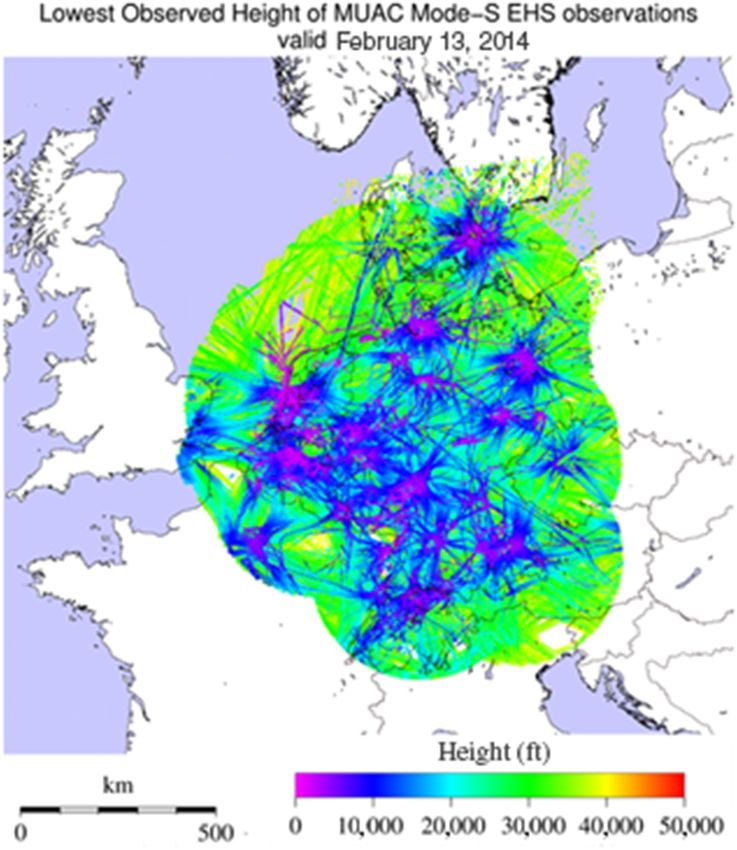
by a function of the difference between observed and simulated assimilated (Arriola et al., 2016) as well as AMVs and Mode-S EHS
reflectivities: winds obtained from air traffic control systems and GNSS radio-
occultations. Last, but not least important, radar reflectivities,
HU exp −Jpo (xi ) pre-processed to relative humidity profiles, are assimilated. These
ypo =
HU
xi (11)
j exp −Jpo (xj )
can be obtained for most European weather radars through
i
the OPERA network (section 4.2.2). In research experiments
Doppler radar radial winds have also been assimilated, aiming for
with
operational implementation. Other observation types revealing
1 encouraging results in DA experiments are radiances from the
Jpo (x) = {yZ − HZ (x)}T RZ−1 {yZ − HZ (x)}, (12) SEVIRI instrument on board the geostationary MSG satellites as
2
well as assimilation of the cloud cover products obtained from
where HZ (x) is the simulated reflectivity and RZ is the observation- the nowcasting SAF.
error covariance matrix. Equation (11) can be interpreted as A crucial challenge for limited-area DA is how to best utilize
one particle filter formulation, in which ‘neighbouring’ vertical information from the larger-scale host model in nested DA.
columns in the first-guess field are treated as prior ensemble ECMWF operational forecasts, with a 6 h lag, provide the LBCs. In
members. Following sensitivity studies, the vicinity of the the baseline HARMONIE-AROME, upper-air DA system spectral
observation has been chosen to be a moving window of 13 mixing of large-scale host model information with smaller-scale
× 13 columns spread uniformly within a 200 km × 200 km HARMONIE-AROME model data is applied in a step prior to
square centred on the observation location. The assumptions upper-air DA (Müller et al., 2017). The characteristic scale of
for the reflectivity observation operator HZ , largely discussed the spectral mixing is dependent on a rather empirically selected
in Wattrelot et al. (2014), were chosen in order to provide a vertically dependent mixing wave number. An alternative, more
good compromise between a realistic simulation (which takes attractive, approach is to incorporate the host model information
into account cold processes and an accurate modelling of the in the cost function through a large-scale error constraint
radar beam) and the need to adapt to the massively parallel code (Guidard and Fischer, 2008; Dahlgren and Gustafsson, 2012)
AROME. Once retrieved, the humidity profiles enter a screening which has been applied for reanalysis purposes, but further
procedure where a specific quality check is done to control refinements are needed.
a posteriori the convergence of the 1D Bayesian inversion. As for
the radial velocities, horizontal spatial thinning is used to reduce 2.2.5. ALADIN/LACE data assimilation
the representativeness errors.
The assimilation of radar reflectivities alone gave a positive Member countries of the ALADIN consortium have taken part in
impact on quantitative precipitation forecasts. Adding Doppler the implementation of limited-area variational DA tools (Fischer
radial winds also improved the quality of the low-level winds. et al., 2005; Bölöni, 2006). The use of upper-air observations in the
c 2018 The Authors and Crown Copyright, Met Office. Quarterly Journal of the Q. J. R. Meteorol. Soc. (2018)
Royal Meteorological Society published by John Wiley & Sons Ltd on behalf of the Royal Meteorological Society.You can also read


