Technical report - Climate Change in Australia
←
→
Page content transcription
If your browser does not render page correctly, please read the page content below

Victorian Climate
  Projections 2019

Technical report
© 2019 State of Victoria
Creative Commons Attribution 4.0 Australian licence (https://creativecommons.org/licenses/by/4.0/)

Updated to correct typological errors 18 February 2020

ISBN 978-1-76077-735-7 (Print)
ISBN 978-1-76077-736-4 (pdf/online/MS word)

Acknowledgements
This scientific assessment and new research has been funded by the Victorian Government Department of Environment, Land,
Water and Planning (DELWP). The authors wish to acknowledge the assistance of the Technical Reference Group, comprising
Dr Rob Vertessy (Chair), Dr Penny Whetton and Dr Karl Braganza. We also wish to acknowledge the members of the User
Reference Group for providing feedback on the project design and resulting products. The authors also wish to thank Rebecca
Harris and Tom Remenyi for allowing us to use the Wine Australia downscaling experiment data sets for this report. Finally, the
authors wish to thank Clare Brownridge, Ramona Dalla Pozza and Alice Bleby for their support while developing this report.

Editorial support: Karen Pearce
Design and layout: Kate Hodge
Citation
Clarke JM, Grose M, Thatcher M, Hernaman V, Heady C, Round V, Rafter T, Trenham C & Wilson L. 2019. Victorian Climate
Projections 2019 Technical Report. CSIRO, Melbourne Australia.

Disclaimer
CSIRO and the State of Victoria advise that the information contained in this publication comprises general statements based
on scientific research. The reader is advised and needs to be aware that such information may be incomplete or unable to be
used in any specific situation. No reliance or actions must therefore be made on that information without seeking prior expert
professional, scientific and technical advice. To the extent permitted by law, CSIRO and the State of Victoria (including their
employees and consultants) exclude all liability to any person for any consequences, including but not limited to all losses,
damages, costs, expenses and any other compensation, arising directly or indirectly from using this publication (in part or in
whole) and any information or material contained in it.
Technical report

Contents
  Executive summary................................................................................ 5
  1. Introduction..................................................................................... 7
      1.1 Background............................................................................................................................................7
      1.2 Climate change in Victoria...................................................................................................................7
      1.3 Why produce new projections?..........................................................................................................9

  2. Methods......................................................................................... 10
      2.1 Climate data sets................................................................................................................................ 10
      2.2 New modelling.................................................................................................................................... 12
      2.3 Area-averaged changes..................................................................................................................... 15
      2.4 Regionalisation................................................................................................................................... 16
      2.5 Application-ready data sets.............................................................................................................. 18

  3. Important features of Victoria’s climate............................................ 19
      3.1 El Niño Southern Oscillation............................................................................................................ 21
      3.2 Southern Annular Mode.................................................................................................................... 21
      3.3 Indian Ocean Dipole.......................................................................................................................... 21
      3.4 Blocking highs..................................................................................................................................... 21

  4. Model evaluation and confidence...................................................... 22
      4.1 Confidence........................................................................................................................................... 22
      4.2 Model evaluation................................................................................................................................ 23
              4.2.1 Temperature..............................................................................................................................................24
              4.2.2 Urban heat island.....................................................................................................................................27
              4.2.3 Average rainfall.........................................................................................................................................28
              4.2.4 Extreme rainfall.........................................................................................................................................29
              4.2.5 Mean sea-level pressure..........................................................................................................................31
              4.2.6 Upper-level wind speed and direction at 850 hPa.............................................................................32
              4.2.7 Summary of CCAM evaluation...............................................................................................................32

  5. Victoria’s changing climate.............................................................. 34
      5.1 Climate features and drivers............................................................................................................ 34
      5.2 Temperatures...................................................................................................................................... 34
              5.2.1 Observed....................................................................................................................................................34
              5.2.2 Near-term temperature change (current to 2030).............................................................................36
              5.2.3 Temperature change for this century...................................................................................................38
              5.2.4 Temperature extremes............................................................................................................................43
      5.3 Rainfall.................................................................................................................................................. 47
              5.3.1 Past changes.............................................................................................................................................48
              5.3.2 Projected change – global and Australia.............................................................................................49
              5.3.3 Projected change – Victoria and sub-regions.....................................................................................51
              5.3.4 Snow...........................................................................................................................................................59
              5.3.5 Rainfall extremes......................................................................................................................................59

                                                                                                                                                                                        iii
Victorian Climate Projections 2019

            5.4 Mean sea-level pressure.................................................................................................................... 62
            5.5 Winds and storms............................................................................................................................... 63
                     5.5.1 Mean winds................................................................................................................................................63
                     5.5.2 Extreme winds...........................................................................................................................................63
                     5.5.3 Storms and lightning...............................................................................................................................64
            5.6 Relative humidity................................................................................................................................ 64
            5.7 Evaporation......................................................................................................................................... 65
            5.8 Fire weather......................................................................................................................................... 65
            5.9 Sea level............................................................................................................................................... 67
            5.10 Step changes....................................................................................................................................... 69

       6. Victoria under the Paris Agreement targets and beyond 2100.............. 71
            6.1 Paris Agreement targets – the ambitious ‘best-case’ scenario.................................................. 71
                     6.1.1 Physical changes in Victoria at 2°C global warming..........................................................................71
            6.2 How we get there matters................................................................................................................. 73
            6.3 Worst-case scenarios......................................................................................................................... 73
            6.4 Change beyond 2100......................................................................................................................... 74

       7. Guidelines for using Victoria’s climate projections.............................. 76
            7.1 Getting started..................................................................................................................................... 77
            7.2 Using climate projections in an impact assessment................................................................... 78
                     7.2.1 Chain of actions........................................................................................................................................78
            7.3 Constructing climate projections – the CSIRO Climate Futures framework........................... 79
                     7.3.1 Sensitivity analysis...................................................................................................................................82
                     7.3.2 Spatial analogues.....................................................................................................................................82
            7.4 Obtaining VCP19 high-resolution climate data............................................................................ 83
            7.5 Further resources................................................................................................................................ 83

       Appendix: Bias plots for model evaluation.............................................. 84
       Shortened forms.................................................................................. 88
       Glossary of terms................................................................................. 88
       References.......................................................................................... 92

                iv
Technical report

Executive summary
This report describes a set of climate projections featuring new high-resolution climate change
simulations for Victoria developed by CSIRO’s Climate Science Centre (CSC), which describe how the
regional climate of Victoria is likely to respond to global warming with different scenarios of human
greenhouse gas emissions. This work was commissioned by the Victorian Department of Environment,
Land, Water and Planning (DELWP) to supplement previous projections of climate change for Victoria and
to develop a tailored climate projections and guidance package for Victoria.

An important consideration when developing regional climate       temperature was 1996 relative to the 1961–1990 baseline.
change projections is to avoid basing the projections on a        Simulations of future warming under plausible greenhouse
single modelling system or an individual line of evidence.        gas emission scenarios are consistent with a 0.5 to 1.3°C
For this reason, it was decided to extend the existing climate    increase in temperature between the 1990s and 2030s. After
change projections information from the Victorian Climate         superimposing natural variability on the global warming
Initiative (VicCI) summarised in (Hope et al. 2017), and          signal, it is possible to observe negligible or even negative
presented in the guidelines for assessing the impact of climate   short-term trends in temperature between 2019 and 2030.
change (DELWP 2016). Those projections drew strongly on           Beyond the next couple of decades, the projected change
statistically downscaled simulations of climate change for        in temperature depends strongly on the greenhouse gas
Victoria and were aimed primarily at water managers. The new      emissions pathway that the world follows. For example,
results presented here feature a dynamically downscaled set       between the 1990s and 2090s, the temperature over Victoria
of simulations based on the Conformal Cubic Atmospheric           is projected to warm on average by 2.8 to 4.3°C under a high
Model (CCAM), as well as drawing on the full range of outputs     emissions scenario or warm by 1.3 to 2.2°C under a medium
from Climate Change in Australia (CCIA) using global climate      emissions scenario. In the case where global warming
models and other climate modelling data sets. For the new         is limited to 2°C, matching aspirations under the Paris
CCAM simulations, six global climate models were downscaled       Agreement, then Victoria is expected to warm by a similar
to 5 km resolution over Victoria. The six high-resolution CCAM    amount, in contrast to many other places in the world that
simulations are based on a subset of the global climate model     will warm by more or less than the global average. The new
simulations recommended by CCIA as representative of the          high-resolution simulations suggest that increases in average
range of projected changes in temperature and rainfall as         temperature can be higher than previously estimated,
well as other climate variables. The regional climate change      especially in spring. This means a hotter ‘worst-case’
projections described in this report combine the results of the   scenario should be considered to manage
new and previous climate model simulations to provide an          risks appropriately.
assessment of plausible changes to the regional climate that
could pose significant risks for the state of Victoria.

The climate of Victoria has been getting warmer, with the
mean annual temperature rising by just over 1°C between
1910 and 2018 according to high quality observations
from ACORN-SATv2. There have been more
warm years than cool years in recent
decades, and the last year
with below-average

                                                                                                               5
Victorian Climate Projections 2019

Victoria is projected to continue becoming drier in the            Caution should always be employed when interpreting the
long term in all seasons except summer, for which models           results of a single climate modelling system until combined
indicate that both increases and decreases in average              with additional lines of evidence and data from other
rainfall are possible. Large rainfall variability at scales from   available models. Nevertheless, the new high-resolution
days to decades is expected to continue. The new regional          downscaling indicates that it is possible for regional daily
climate model simulations are broadly consistent with              average temperatures to increase up to 1°C more than was
previous climate projections across Victoria as a whole,           projected by the global climate models in some seasons
except for the summer and autumn signature where the new           and regions. For example, for Gippsland in spring under
simulations show high agreement on a projected decrease            a high emissions scenario around the end of the century,
whereas previous dynamical downscaling indicated an                the upper range of daily average temperature change from
increase (Grose et al. 2015a; Hope et al. 2015b; Timbal et         global models is 3.9°C. In contrast, the high-resolution
al. 2015; DELWP 2016; Hope et al. 2017; Potter et al. 2018).       simulations suggest the change could be up to 5.1°C. This
The projection of autumn and summer rainfall in the new            result is considered plausible as the regional model captures
dynamical downscaling agrees more with the global climate          the feedback from the drier landscape under hotter daytime
model projections and statistical downscaling, as well as          temperatures, and better represents the weather effects
the recent observed decrease in autumn rainfall, leaving the       from the finer resolution of the boundary between land and
previous downscaling as exceptions. However, there is not          oceans. Extreme daily maximum temperatures are projected
sufficient evidence to reject any set of results as implausible    to increase by as much as twice the increase in the average
and this reinforces the need to consider a range of models         maximum temperatures. The new high-resolution modelling
and multiple lines of evidence when assessing projected            also indicates that large increases in winter extreme daily
change in the regional climate. The new high-resolution            maximum temperatures are possible. Another important
modelling identifies a greater projected decrease in the           insight from the new regional projections for Victoria is that
annual-averaged rainfall than in the surrounding regions           the new modelling indicates that rainfall and inflows over
– on the windward (western) slopes of the Australian Alps          the Australian Alps and in the Murray River catchments may
(primarily in the Ovens Murray region) in autumn, winter and       be affected to a greater degree than has been previously
spring compared to the surrounding regions.                        expected under high greenhouse gas emission scenarios.

Consistent with previous studies of projected regional             The new regional climate projections for Victoria described
climate change, extreme events such as heatwaves, bushfires        in this report indicate that climate change poses a serious
and extreme rainfall are expected to continue to become            risk for Victoria. The data in this study are intended to
more frequent in the decades to come. The intensity and/           support planning and policy decisions made by the Victorian
or frequency of past 1-in-20-year extreme daily rainfall is        Government and community as well as being used by
expected to increase, even in areas where average rainfall is      scientific researchers to better understand the consequences
expected to decline. The number of fire days are expected          of global climate change. Regional climate projections will
to increase under most global warming scenarios, with a            continue to be improved and enhanced as new climate
larger increase in fire days for alpine regions. The results       change information becomes available but building on
of the new high-resolution modelling are consistent with           foundations developed in this study as well as previous
more favourable conditions for thunderstorms under                 projects such as VicCI, and findings coming out of the
global warming.                                                    current Victorian Water and Climate Initiative. It is important
                                                                   to combine future climate projections with knowledge of
        New high-resolution climate modelling has produced         climate exposure and vulnerability, as well as adaptive
               several important new insights about the            capacity to assess what a changing climate means to any
                        possible future climate of Victoria.       given question or sector.

               6
Technical report

1. Introduction
This chapter gives the background to the project, a quick introduction to how climate change has been
assessed at global, Australian and state levels, and the motivation for producing new work at this time.

1.1 Background                                                     An example of using the new projections as a complement to
                                                                   previous work can be shown for water management. Victoria
In 2018 the Victorian Department of Environment, Land,
Water and Planning (DELWP) commissioned CSIRO’s                    has a detailed water management plan to manage water
Climate Science Centre (CSC) to undertake new high-                resources under a changing climate https://www.water.
resolution climate modelling and produce a tailored climate        vic.gov.au/water-for-victoria. The risk management plan
projections and guidance package for Victoria. The package         includes a consideration of a range of projected changes
was commissioned to supplement the national projections            in rainfall and evaporation by the end of the century, as
at www.climatechangeinaustralia.gov.au (CCIA), the Victorian
                                                                   well as the resampling of observations to produce severe
Climate Initiative (VicCI) and other projects supported by the
Victorian Government. The package is titled Victorian Climate      hypothetical droughts as a worst-case scenario planning
Projections 2019 (VCP19), and this technical report is part of     exercise for the coming years. The new VCP19 modelling has
that package.                                                      produced additional insights into the plausible change in
                                                                   rainfall over mountains, so provides a new dry case for the
VCP19 has developed a new set of high-resolution regional
                                                                   long-term future on the western slopes of the ranges that
climate simulations for Victoria using alternative methods
from that used in VicCI and other previous studies (CSIRO          is consistent with the previous resampling method used to
and Bureau of Meteorology 2015; Hope et al. 2015a; Hope            consider the near-term changes in climate. In this way, the
et al. 2017; Potter et al. 2018). VCP19 is designed to be          new VCP19 projections add to the existing knowledge base
complementary to VicCI and CCIA projections by adding new          rather than replace it.
regional insights into future climate change and providing
supplementary information and additional guidance to               DELWP and the Victorian Government supported the
assessing climate change impacts. Projected changes in the         production of the Climate-ready Victoria set of products in
climate can be better understood by using multiple lines
                                                                   20161. These products are based on the national climate
of evidence and data where possible. For this reason, the
                                                                   projections reports and model inputs aggregated for the
new modelling results are put in context of previous work
wherever possible, both in terms of identifying messages           same regions used in VCP19. The messages and conclusions
that are consistent between the different methods and              of Climate-ready Victoria are still current and relevant, and as
identifying any new projected changes and regional insights        for VicCI, the new VCP19 work presented here complements
from the new modelling. Differences between the different          and adds to this work rather than replaces it.
high-resolution climate data sets generally indicate the range
of different possible changes to Victoria’s future climate that
can occur consistent with global warming (e.g. changes in          1.2 Climate change in Victoria
extreme weather). Such differences in climate model results
                                                                   Victoria’s changing climate presents a significant challenge
can be used to identify physical processes that underpin
                                                                   to individuals, communities, governments, businesses and
the projected changes and generally help to improve our
understanding of the future climate. New insights from the         the environment. Like the remainder of Australia, Victoria
climate projections are noted in the executive summary and         has already experienced increasing temperatures (Figure 1),
highlighted throughout the report.                                 shifting rainfall patterns and rising oceans.

1 https://www.climatechange.vic.gov.au/information-and-resources

                                                                                                                    7
Victorian Climate Projections 2019

The Intergovernmental Panel on Climate Change (IPCC)              Victoria is represented in these national projections as part
Fifth Assessment Report (IPCC 2013) rigorously assessed           of the Murray Basin (Timbal et al. 2015) and Southern Slopes
the current state and future of the climate system, making        (Grose et al. 2015a) clusters.
several important conclusions:
▶▶   Greenhouse gas emissions have markedly increased             The 2018 State of the Climate (Bureau of Meteorology and
     because of human activities.                                 CSIRO 2019) reports that:

▶▶   Human influence has been detected in warming of the          ▶▶   Australia’s average temperature has increased by more
     atmosphere and the ocean, in changes in the global                than 1°C since 1910
     water cycle, in reductions in snow and ice, in global mean   ▶▶   extreme heat events have increased in frequency
     sea-level rise, and in changes in some climate extremes.
                                                                  ▶▶   rainfall in southeast Australia has declined by around
▶▶   It is extremely likely that human influence has been the
                                                                       11% in the April to October period since the late 1990s
     dominant cause of the observed warming since the mid-
     20th century.                                                ▶▶   extreme fire weather has increased in frequency
▶▶   Continued emissions of greenhouse gases will cause                and duration
     further warming and changes in all components of the         ▶▶   sea levels have risen leading to increased inundation risk.
     climate system.
                                                                  Victoria has its own interests regarding climate change, risk
In recognition of the impact of climate change on the
                                                                  and adaptation. For these reasons, in recent years the
management of Australia’s natural resources, the Australian
                                                                  Victorian Government has supported climate research,
Government funded CSIRO and the Australian Bureau of
                                                                  climate projections, risk and adaptation work with a local
Meteorology (BOM) to develop tailored climate change
projections reports for each of eight natural resource            focus. On the research and projections side, the South East
management (NRM) ‘clusters’ (i.e. clusters of existing NRM        Australia Climate Initiative (SEACI) and the Victorian Climate
regions). These projections, Climate Change in Australia          Initiative (VicCI) programs have generated science research
(CCIA), were released in 2015 and provide guidance on the         and communication products targeted at Victoria and the
changes in climate that need to be considered in planning.        Murray Basin.

                                                                                                   Figure 1. Average annual near-
                                                                                                   surface (2 m) temperature of
                                                                                                   Victoria 1910 to 2018 relative to
                                                                                                   the 1961–1990 baseline average.
                                                                                                   Panel on the bottom shows
                                                                                                   ‘climate stripes’ where each
                                                                                                   stripe represents the temperature
                                                                                                   anomaly of one year, reds
                                                                                                   indicate temperatures above the
                                                                                                   1961–1990 average and blues,
                                                                                                   below average (ACORN-SATv2
                                                                                                   data set, scale ranges from 1.5 to
                                                                                                   +1.5°C, methods of Ed Hawkins)

               8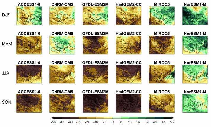
Technical report

1.3 Why produce new projections?                                 These emissions scenarios were chosen to explore some of
                                                                 the larger potential changes in the Victorian climate that can
Since climate change operates over longer scales, climate
                                                                 arise under different greenhouse gas emission scenarios. The
projections do not need to be updated daily or monthly like      use of the two greenhouse gas emissions scenarios in the
weather or seasonal forecasts. However, as our observations      high-resolution modelling was made possible by combining
of the climate continue, our climate knowledge continues to      the resources of the VCP19 projections project with an
improve, models improve, and needs for climate information       existing project undertaken by Wine Australia and lead by
and projections continues to evolve. This means the              researchers at the University of Tasmania. Both sets of high-
credibility and salience of projections can be higher over       resolution climate simulations were performed concurrently
time, so it is advisable to update climate assessments and       with common model configuration and methods, allowing
projections when appropriate.                                    for a broader assessment of potential changes to climate
                                                                 than would otherwise be possible. This technical report
Milestones for developing projections include the release of
                                                                 presents the results of this work at the spatial scale of the
IPCC assessment reports, and the release of new coordinated
                                                                 state of Victoria and sub-regions within Victoria.
climate modelling ensembles under the Coupled
Model Intercomparison Project (CMIP) structure. These            The outputs from the VCP19 project are available to the
international milestones then influence the development of       Victorian Government, broader community and the scientific
projections at the national, state and local level. The most     community to improve understanding and application of
recent IPCC assessment report was released in 2012/13 and        climate projections. The outputs of VCP19 are:
this draws on the latest round of coordinated global climate
                                                                 ▶▶   this technical report – aimed at scientists
models known as CMIP5 released in 2011/12, among many
other lines of evidence. The CCIA climate projections draw       ▶▶   10 regional reports – aimed at non-scientists
on the science and model simulations from this period,           ▶▶   projections and data for medium (RCP4.5) and high
as well as drawing on high-resolution climate modelling               (RCP8.5) scenarios of future greenhouse gas emissions
based on the CMIP5 outputs. VCP19 uses the same CMIP5
outputs, as well as new high-resolution climate modelling,
                                                                 ▶▶   projections of Victoria’s climate under the Paris
combined with subsequent research and observations.                   Agreement target of 2°C global mean temperature
                                                                      increase compared to the pre-industrial era
VCP19 is expected to be current until at least the release of
the sixth IPCC assessment and CMIP6 in 2022, and for some        ▶▶   good practice guidance for how to make best use of the
time beyond as the new research and modelling will take               new projections and data sets
time to be translated to local issues. Future climate research   ▶▶   data sets of projected regional changes for 12
and modelling are likely to incrementally improve our
                                                                      climate variables (including four measures of climate
understanding and refine our projections of climate change;
                                                                      extremes) for 10 regions on annual, seasonal and
however, this work is unlikely to change the fundamental              monthly time scales
understanding of climate change in Victoria. This means the
VCP19 projections are expected to be relevant after 2022,        ▶▶   gridded (5 km) and town-based ‘application-ready’
with some contextualising of the results consistent with the          data sets for 10 climate variables for annual to
future research.                                                      daily time scales
                                                                 ▶▶   gridded (5 km) change data sets for 11 climate variables
Global climate model data is available for a range of future          for annual to daily time scales
greenhouse gas emission scenarios agreed to by the
international climate research community. However, due to
                                                                 ▶▶   gridded (5 km and 50 km) output for six high-resolution
                                                                      climate model experiments with more than 20 climate
limitations on modern supercomputing resources, the new
                                                                      variables for up to hourly time scales
high-resolution climate modelling focused on a medium
emissions scenario (RCP4.5, see the glossary of terms at the     ▶▶   new functionality on the Climate Change in Australia
end of this report) and a high emissions scenario (RCP8.5).           website, providing access to the new data and products.

                                                                                                                    9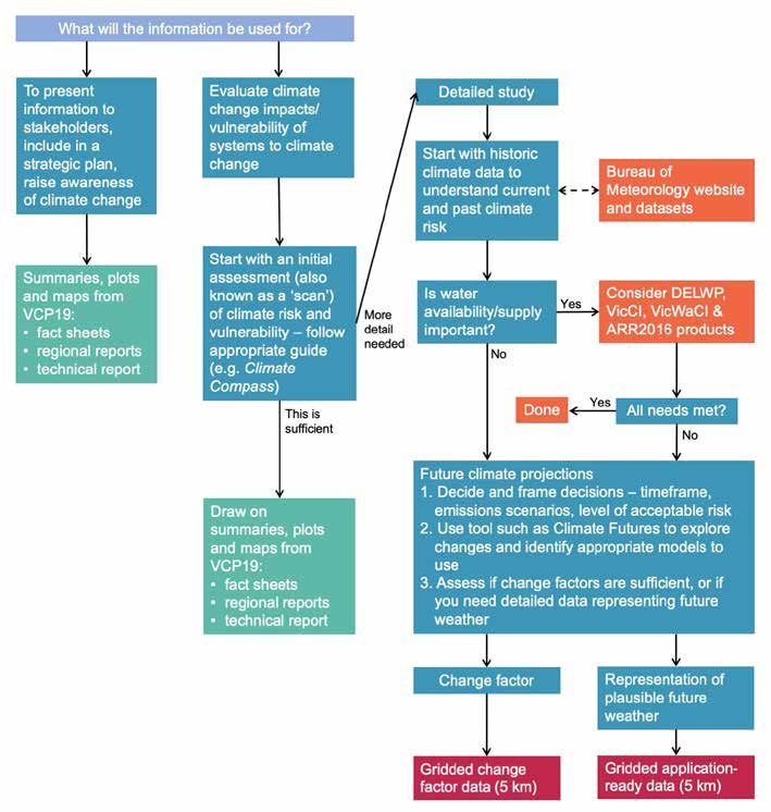
Victorian Climate Projections 2019

2. Methods
This chapter explains the data sets, models and analysis techniques used to produce the VCP19 climate
projections. The chapter outlines the existing set of previous modelling considered in VCP19 and the process to
produce the new fine-scale regional climate model (RCM) simulations of the Victorian climate. The chapter also
describes the regions considered, and how changes are calculated and presented for the regions.

2.1 Climate data sets                                               trapped in the Earth system by the increased concentrations
                                                                    of greenhouse gases. A higher number associated with an RCP
When developing regional climate projections for Victoria, it
                                                                    results in a warmer climate and more severe impacts on the
is important that multiple and reputable lines of information
                                                                    environment. RCP2.6 is the greenhouse gas emission scenario
and evidence are examined and considered such as
                                                                    used by the GCM development teams that is the closest to
observations, trends, global climate models of future climate
                                                                    that required to meet the Paris Agreement targets discussed
and higher resolution regional climate models. This approach
                                                                    in Chapter 6. RCP4.5 and RCP8.5 are often a focus for climate
ensures that the different possible future climates simulated
                                                                    projections as they have been interpreted as medium and
by climate models are considered and an appropriate level
                                                                    high emissions scenarios, respectively.
of confidence is assigned to different outcomes of global
warming. Without a documented case, no set of outputs
                                                                    The GCMs contributing to the CMIP experiments provide
should be considered superior to all others and used in
                                                                    the most diverse set of independent model data sources for
isolation, although agreement between different model
                                                                    developing climate projections. However, a limitation of GCM
ensembles can be a source of confidence in the results. It is
                                                                    data sets is that the complexity of the modelling combined
also important to consider some of the more extreme model
                                                                    with limitations on supercomputing hardware results in
simulation results if they are credible, given the significant
                                                                    GCMs typically having a grid-box resolution of 100 to 200 km.
impacts that could occur if that model projection was realised
                                                                    This means that mountains and coastlines are not always
in our future climate. Developing regional climate projections
                                                                    well resolved, urban areas can be neglected, and certain
is a process of collecting all available historical and simulated
                                                                    atmospheric phenomena can be poorly resolved (e.g. storms).
future climate change information and interpreting that
                                                                    Downscaling techniques are often employed to supplement
information to understand the probable and possible regional
                                                                    some of the missing information needed for regional
outcomes of global warming.
                                                                    projections of climate change that is not directly available
Global climate models (GCMs) are our best source of                 from the GCMs.
information regarding how increasing greenhouse gas
concentrations can affect the global climate of the Earth.          Downscaling can use a wide variety of techniques, all with
These GCMs are computer software models that couple                 various strengths and weaknesses (Ekström et al. 2015). In
various components of the Earth system, including                   general, downscaling attempts to interpret regional changes
atmospheric processes, land processes, oceans, sea-ice,             in climate that are poorly resolved in the GCM simulations.
aerosol feedbacks and carbon cycle feedbacks. By using              Two popular approaches to downscaling climate models are
prescribed scenarios of greenhouse gas emissions, it is             statistical downscaling and dynamical downscaling. Statistical
possible to estimate how quickly the Earth system can warm          downscaling, as used for the Victorian Climate Initiative (VicCI),
and some of the responses to this warming by the different          relies on relationships between large-scale atmospheric
Earth system components (e.g. melting of sea-ice). To aid with      behaviour and the local response in weather. Often statistical
the development of climate change projections, the different        downscaling is informed by historical observation records,
GCMs all contribute to the Coupled Model Intercomparison            from which the large-scale and local-scale relationships can
Project (CMIP, with the current generation being CMIP5 and          be derived. In comparison, dynamical downscaling techniques
the new CMIP6 experiment being underway at the time of              rely on a computer simulation of different atmospheric and
writing). For the CMIP5 generation of GCMs, greenhouse              land-surface processes, in a similar way to how the GCMs
gas emission scenarios are described by representative              model the atmosphere. However, dynamical downscaling
concentration pathways (RCPs). The RCPs comprise RCP2.6,            focuses its computing resources to better spatially and
RCP4.5, RCP6 and RCP8.5, where the number after the RCP             temporally resolve a small region, at the expense of resolving
indicates the increase rate of energy (e.g. stored as heat)         the rest of the globe. Dynamical downscaling models also

               10
Technical report
usually focus on the atmospheric and land-surface modelling, experiment framework. The New South Wales Government
neglecting ocean and sea-ice components of the GCMs. has previously commissioned a dynamical downscaling of
Combining the results of statistical (e.g. VicCI) and dynamical the regional climate for their state at 10 km resolution, which
methods can often be useful for developing regional climate is known as the NSW and ACT Regional Climate Modelling
projections, since the statistical approach relies on historical (NARCLiM) project, which overlaps with the Victorian region
data to interpret regional changes in climate, whereas the and therefore contributes towards the Victorian regional
dynamical approach relies on computer simulations of projections. Another relevant data set for this study is the
atmospheric processes at finer spatial-scales than is practical Benefits of Reduced Anthropogenic Climate Change (BRACE),
for the GCMs to simulate. This leads to different assumptions which is a project looking specifically at the reduced impacts
behind the downscaling technique, which can be best of lower emissions scenarios compared to higher ones
understood by combing multiple sources of downscaling (Sanderson et al. 2018). This includes climate change under
when developing regional projections. The learning from the Paris Agreement global warming targets of 1.5 and 2°C
comparing these different downscaling techniques is since pre-industrial times, partly produced to inform the IPCC
discussed further in Chapter 5. Special Report on 1.5°C (IPCC 2017). The project included
the production of a global climate model medium ensemble
An example of an important downscaled data set for Victoria of the Community Earth System Model (CESM) where global
is the statistically downscaled 5 km resolution data sets warming plateaus at each target, titled BRACE1.5. The
developed for VicCI. This climate data is already being used ensemble features 15 climate simulations meaning that
within the Victorian Government and water corporations and variability is well sampled but is dependent on a single global
is important for framing new and future climate modelling. climate model.
Another source of downscaled climate data for Australia is
the Coordinated Regional Climate Downscaling Experiment The Victorian Climate Projections 2019 project draws on a
(CORDEX) regional climate model inter-comparison range of available data sets in addition to the new high-
experiment (http://www.cordex.org/). CORDEX provides resolution modelling undertaken specifically for Victoria using
50 km resolution climate data for the Australasia region the Conformal Cubic Atmospheric Model (CCAM) described in
(including Australia, New Zealand and neighbouring islands), the following section. The climate data sets used to develop
using different climate modelling systems within a common regional projections for Victoria are summarised in Table 1.
Table 1. Climate projection data sources drawn on for the Victorian Climate Projections 2019 (VCP19) development
Data set Provenance Resolution Contribution to VCP19
VCP19 CCAM Focus on Victoria; based on CMIP5, 5 km Primary high-resolution data source (50 km
RCP4.5 and RCP8.5 version also used for national context)
GCMs from the Coupled International; up to 42 models; 60–200 km Source of host models for CCAM
Model Intercomparison source for IPCC Fifth Assessment downscaling; key source of CCIA data sets
Project phase 5 (CMIP5) Report (2013)
Climate Change in Australia Australia-wide (CMIP5 based); Application-ready Key data source; critical context for
(CCIA)1 published 2015 5 km; change data: Victorian projections; includes earlier 50
60–200 km km CCAM data; source of Australian model
evaluation information; guidance material
Bureau of Meteorology Contributed to CCIA and VicCI data 5 km Context for VCP19
Statistical Downscaling sets
Model (BOM-SDM)1,2
NSW and ACT Regional Focus on NSW, also covers Victoria; 10 km (some data at Context for VCP19; comparison of higher
Climate (NARCLiM)3 based on CMIP3, SRES A2 only higher resolution) emissions scenarios (A2)
Benefits of Reduced International Global and Victoria New application to Australian context;
Anthropogenic Climate future climate under the Paris Agreement
Change (BRACE)4 targets of 1.5 & 2.0°C warming
1 https://www.climatechangeinaustralia.gov.au/en/climate-projections/about/modelling-choices-and-methodology/
2 http://www.bom.gov.au/research/projects/vicci/
3 https://climatechange.environment.nsw.gov.au/Climate-projections-for-NSW/About-NARCliM
4 http://www.cgd.ucar.edu/projects/chsp/brace1.5.html
11Victorian Climate Projections 2019
All currently used, or otherwise current generation climate High-resolution dynamical downscaling of global climate
model outputs have been considered, except for the Climate simulations can result in improved modelling of regional
Futures for Tasmania data sets that are not included here as: climate where there is complex orography, such as
mountains or coastlines that were poorly resolved by the
▶▶ they were made using the previous generation (CMIP3) of
host global climate model. The higher-resolution dynamical
global climate model inputs
downscaling can also resolve local features such as urban
▶▶ they were developed using a previous version of heat islands due to the ability to include urban materials
the CCAM model and energy use in the simulation. Regional climate models
▶▶ the winter rainfall projection for southeast mainland may also provide better simulation of variability in winds,
Australia is different from host models (the global climate temperature and rainfall, through better resolution of
models used as input) due to a model-specific effect atmospheric processes (e.g. clouds, boundary layer mixing,
that means the results may not be representative of the etc.). Consequently, certain types of extreme weather such
broader range of projections. as storms and strong winds are usually better represented
by the regional climate models than for the lower resolution
global climate models. Dynamical downscaling has been
2.2 New modelling
used to produce transient data sets of projected regional
Although there are a number of existing climate data climate change (e.g. from 1960–2100) rather than time slices
sets described in the previous section, climate change (e.g. 1986–2005, 2041–2060 and 2081–2100) which helps with
simulations for Victoria at resolutions below 10 km were assessing the progression of change. A possible weakness of
limited to statistically downscaled data sets that were used standard dynamical downscaling techniques is that errors in
for VicCI. Therefore, it was decided that new dynamical the GCM simulation may undermine the performance of the
downscaling at a resolution of 5 km could be beneficial RCM simulation. For this reason, it is common for dynamical
when developing projections for Victoria, since the downscaling experiments to attempt to address GCM biases
dynamical downscaling employs different assumptions and and minimise their impact on the RCM simulation (e.g.
techniques to statistical downscaling, so including them Katzfey et al. 2016).
provides a more diverse and independent set of modelling
approaches to inform the predicted changes to the regional For the new VCP19 high-resolution climate simulations,
climate. The new high-resolution dynamical downscaling CSIRO’s CCAM was used for dynamically downscaling GCM
is not a replacement for the existing VicCI data sets, nor data sets (McGregor 2005; McGregor and Dix 2008). CCAM has
a replacement for the GCM data sets. Rather, the new been used for numerous regional climate modelling projects
simulations are intended to provide an additional source of in Australia and overseas, including the NRM projections
information and data that can help strengthen conclusions for Australia, Climate Futures for Tasmania, High-resolution
drawn from existing data sets, shed new insights into some Climate Projections for Queensland and Climate Projections
regional climate phenomena, and help define levels of for the Australian Alps. CCAM is also contributing to the
confidence in the projected regional consequences of global CORDEX intercomparison experiment and is used in South
climate change. Africa, New Zealand, South East Asia and the Pacific. The
CCAM source code is freely available for scientific researchers
There is flexibility in how a dynamical downscaling (https://confluence.csiro.au/display/CCAM/CCAM).
experiment is undertaken, but in general the regional climate
models (RCMs) used for dynamical downscaling adhere to CCAM has a variable resolution global grid that can be
some basic principles: focused over a region of interest (see Figure 2). This means
▶▶ The RCM includes information from the GCMs to the region of interest can be simulated at high resolution,
determine the large-scale changes to the oceans and while still maintaining a lower resolution simulation of
Earth system as well as the rate of global warming. the entire globe. This is different to the more traditional
approach used by RCMs based on a limited area simulation.
▶▶ The RCM includes mountains, coastlines, urban areas Limited area climate models only simulate the climate for a
and other details at the surface that are poorly resolved
region, often defined by a rectangle, and therefore require
by the GCMs.
atmospheric data to be supplied from a GCM at their lateral
▶▶ The RCM improves the representation of atmospheric boundaries that represent the edges of the limited area
physical processes that are relevant for the spatial-scales simulation. Since CCAM does not have lateral boundaries,
being simulated. it can avoid problems arising from the prescription and
12Technical report
interpolation of GCM data at the boundaries of limited area
models. Another feature of CCAM is its use of the Community
Atmospheric Biosphere Land Exchange (CABLE) land-surface
model (Kowalczyk et al. 2013) and the Urban Climate and
Energy Model (UCLEM) (Thatcher and Hurley 2012; Lipson
et al. 2018). These sub-models were developed to better
represent Australian conditions, with the UCLEM model
initially developed to represent the climate of Melbourne,
including the urban heat island discussed in section 4.2.2.
Thirdly, CCAM can operate as a global atmospheric climate
model, which allows us to modify the ocean temperatures
simulated by GCMs to reduce potential GCM biases that
can be introduced into the regional simulation. Although
limited area climate simulations also attempt to correct
biases in their lateral boundary conditions, these corrections
can be complex and non-linear due to the way different
atmospheric variables interact with each other such as
temperature, moisture, clouds, wind, aerosols, etc. CCAM
avoids this problem by using a global simulation where
Figure 2. The CCAM variable resolution global grid, focused
the CCAM physical and dynamical processes can internally
over Victoria
resolve the changes arising from correcting GCM biases.
downscaling experiments such as NARCLiM, where possible.
It should be stressed that regional climate simulations do It is then possible to see if the CCAM simulations are an
not necessarily improve all aspects of a climate simulation outlier of the existing sources of climate change information
and can feature new biases or errors. Also, different and to assign a level of confidence in the CCAM projections.
dynamical downscaling models produce different Care is taken to separate the regional changes in climate
simulations of the future climate, making it more difficult to simulated by CCAM from the larger-scale changes in climate
provide certainty in the production of climate change where possible. For example, the simulated change in
projections. Regional climate models rely on the same rainfall by the high-resolution modelling may be modified
atmospheric physical parameterisations that are used in by the presence of a mountain range that was not resolved
global climate models and can be prone to the same errors in the GCMs, and the simulated change may be supported
due to the imperfect understanding of the atmosphere. Most by a known physical process or mechanism that explains
regional climate models are atmosphere-only models and the regional model projection. There may then be more
do not include feedbacks with the ocean, which can be confidence in generalising the simulated regional change
important for simulating the climate along coastlines. For in rainfall for regional projections, independently of the
VCP19, CCAM was configured in an atmosphere-only model, larger scale changes found in the individual regional climate
due to the CCAM ocean model being under development. simulations.
The reduction of GCM ocean temperature biases also
weakens the relationship between the downscaled climate As well as avoiding using a single source of data for
and the projections of the host GCM, reducing the diversity in developing regional projections for Victoria, it is also
independent sources of climate model data sets. important to downscale multiple GCM simulations of the
future global climate to better represent different possible
All climate models and downscaling techniques include regional changes in climate. This is so that the projected
different assumptions in their design and hence no single changes in the regional climate as simulated by CCAM are
model should be considered a definitive prediction of more consistent with the range of different projections of
the future climate. This principle applies to the CCAM global climate models. This is important when assessing
dynamically downscaled results provided in VCP19, since the range of probable and possible future climate scenarios
CCAM still represents a single modelling system. Therefore, for the regional projections in Chapter 5. Six GCMs were
when discussing the projections of future climate, the CCAM chosen for downscaling by CCAM as listed in Table 2, which
results will be presented in the context of existing GCM were selected from the eight-model subset identified for
results, VicCI statistical downscaling and other dynamical the CCIA projections. These selected GCMs demonstrated
13Victorian Climate Projections 2019
high simulation skill and are representative of the ranges of There are two stages to CCAM downscaling. The first stage is
projected change for Australia. The six models were chosen to simulate the global atmosphere at 50 km resolution, with
to represent a range of climate warming that was consistent the sea surface temperatures (SSTs) taken from the host GCM
with the range of projections made by the CMIP5 ensemble after bias correction of the mean and variance (Hoffmann et
of GCMs, including both drier and wetter future climates, as al. 2016). These simulations run continuously from 1960 to
well as having realistic representations of large-scale drivers 2100, although the historic period (up to 2005) is common for
of the Australian climate (e.g. ENSO, monsoons, etc.). In both RCP4.5 and RCP8.5. The 50 km simulations represent
this way, the six models downscaled can be considered a a reconstruction of the atmosphere after removing biases
combination of higher quality global climate models as well introduced by the GCM SST bias, but to not include any
atmospheric information directly from the host GCM. The
as a sufficient cross-section to represent the broad range of
second stage is to nest a 5 km resolution simulation, focused
global climate model projections for Australia.
over Victoria, using CCAM’s stretched grid within the 50 km
In addition to downscaling the six GCM projections of the global simulation. The 5 km simulation is guided at large
future climate, CCAM also downscaled the ERA-Interim spatial scales by the 50 km simulation using a scale-selective
reanalysis. A reanalysis is produced using data assimilation filter (Thatcher and McGregor 2009) but adds considerable
detail in surface features (e.g. mountains, coasts, urban heat
techniques to incorporate meteorological and ocean
islands, vegetation, etc.) as well as providing some better-
observations of the weather into a global atmospheric
resolved atmospheric processes compared to the GCM (e.g.
simulation. The atmospheric variables are then adjusted to
extreme rainfall). The use of bias-corrected GCM SSTs has
ensure that the global simulation is as consistent with the
significant implications for the downscaling process. Since
observations as possible, while still following the governing
the GCM SSTs are modified and the global atmosphere is
geophysical equations that describe the functioning of the
reconstructed, then the downscaled CCAM data sets can
atmosphere. The assimilation of observations in reanalyses
differ in their projections from the host GCM. As a result,
that are not available to the climate GCMs (which are care is taken to separate the regional-scale projections from
designed to simulate a future climate where the observations the larger-scale projections of the CCAM 50 km simulations.
do not exist) results in reduced simulation errors for the These differences do not necessarily mean that the CCAM
present climate. Hence downscaling of reanalyses is a useful projections are incorrect, rather the projections are
way to evaluate the downscaling performance of CCAM for influenced using a single CCAM-based downscaling process
the present climate. When downscaling climate GCMs for and should be interpreted in the context of the CMIP5 GCM
the future climate, CCAM was run from 1960 to 2100, for two ensemble and other downscaled data sets. A visualisation of
representative concentration pathways (van Vuuren et al. the grid spacing and surface height in each stage shows the
2011): RCP4.5 and RCP8.5. increasing detail through downscaling (Figure 3).
Table 2. The historical reanalysis model and six global climate models used as host models for downscaling over Victoria using
CCAM. The relevance of global climate model is based on Climate Change in Australia.
Model/reanalysis name Relevance for VCP19 projections
ERA-Interim (reanalysis) Reanalysis product that is useful when evaluating dynamical downscaling in the present climate.
ACCESS 1-0 A hot, dry model in the south of Victoria.
Representative of the consensus of GCM projections in northern Victoria.
CNRM-CM5 Representative of the consensus of GCM projections over Victoria, particularly in the north.
GFDL-ESM2M Often a hot, dry model for Victoria.
HadGEM2-CC Often a hot, dry model for Victoria.
MIROC5 Often a low warming, wet model for Australia and Victoria.
NorESM1-M Often a low warming, wet model for Victoria, especially in the south.
14Technical report
Figure 3. Topography of Southeast Australia in a typical GCM resolution (about 150 km), intermediate downscaling using CCAM
(50 km) and high-resolution downscaling using CCAM (5 km), the height scale extends to 2000 m above sea level.
It should be noted that the final report for the VicCI project representative GCMs, such as how regional influences might
(Hope et al. 2016) raised some important questions modify the rainfall compared to the GCM simulation. For this
regarding the use of downscaling approaches for developing reason, regionally dependent projections of the model are
climate change projections. They observed a marked from the large-scale changes that arise from a combination
divergence in the results of the statistically downscaled of changes in ocean temperatures simulated by different
models compared with the dynamically downscaled models GCMs but interpreted by a single CCAM atmospheric model.
that they examined. This behaviour also occurs for the Chapter 5 contains examples of how the CCAM results can
CCAM dynamical downscaling described in this report. All modify some regional aspects of the GCM simulations, so
downscaling models will have broadscale biases and errors that the results can be interpreted in the broader range of
in their simulation of the regional climate that are associated GCM projections.
with that model. The different biases of downscaling models
can be illustrated by comparing the different downscaling
2.3 Area-averaged changes
data sets, although the model with the smallest biases is
usually unknown. Unless there is a physical explanation In line with international practice (IPCC 2013a), a time-slice
that can clarify why an individual downscaling approach approach is used to compute future change relative to
is incorrect, then no single downscaling modelling system an historic baseline (see Figure 4). This method involves
can be preferred over any other downscaling technique. In calculating the difference between a climate model’s
this way, the CCAM downscaling experiments presented in future and historic values (each averaged over 20 years) for
this report are intended to enhance the amount of climate a given emissions scenario and time-period. The historic
modelling data that can be used to develop regional baseline period used for this calculation was the 20-year
projections, rather than be considered a superior data period, 1986–2005. This is consistent with the IPCC’s Fifth
set to other downscaling techniques. There are examples Assessment Report (IPCC 2013a) and the CCIA projections
discussed later in this report where CCAM will provide some (CSIRO and Bureau of Meteorology 2015).
important insights into future changes in Victoria’s climate,
but these insights are most effective when their conclusions
are reinforced by the other downscaling techniques.
It is important to note that dynamically downscaling to
higher resolution does not necessarily eliminate errors from
the host GCM’s climate simulation. Rather, the dynamically
downscaled simulations can supplement and extend
projections made by the GCM. For example, the CCAM
dynamical downscaling can better represent the mean
rainfall near mountains, and better represent extreme rainfall
compared to the host GCMs. The CCAM output should not be
used independently of the GCM results, which give a much Figure 4. Time-slice method: by computing the difference
larger ensemble of future climate change for Victoria, but between the model’s future temperature and past values, any
rather be used to better understand the projections of six inherent bias in the model is removed.
15You can also read