Classifying user information needs in cooking dialogues - an empirical performance evaluation of transformer networks
←
→
Page content transcription
If your browser does not render page correctly, please read the page content below
Classifying user information needs in
            cooking dialogues –
  an empirical performance evaluation of
           transformer networks
Masterarbeit im Fach Digital Humanities am Institut für Information und Medien,
                         Sprache und Kultur (I:IMSK)

    Vorgelegt von: Patrick Schwabl
    Adresse: Hemauerstraße 20, 93047 Regensburg
    E-Mail (Universität): patrick.schwabl@stud.uni-regensburg.de
    E-Mail (privat): patrick-schwabl@web.de
    Matrikelnummer: 1740937
    Erstgutachter: Prof. Dr. Bernd Ludwig
    Zweitgutachter: PD Dr. David Elsweiler
    Betreuer: Prof. Dr. Bernd Ludwig
    Laufendes Semester: 3. Semester M.A. Digital Humanities
    Abgegeben am: 04.04.2021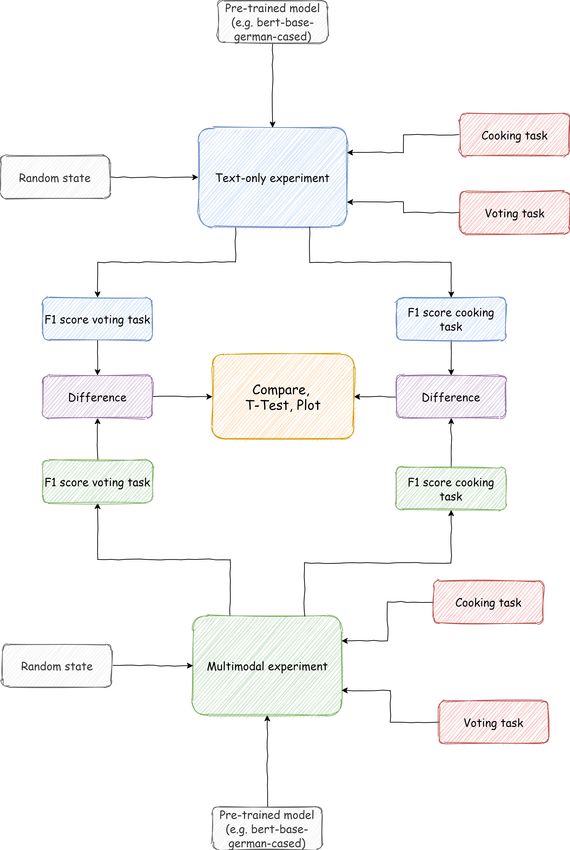
Abstract
In this master’s thesis, I carry out 3720 machine learning experiments. I want to
test how transformer networks perform in a dialogue processing task. Transformer
networks are deep neural networks that have first been proposed in 2017 and have
since rapidly set new state of the art results on many tasks. To evaluate their
performance in dialogue classification, I use two tasks from two datasets. One comes
from a dialogue; the other does not. I compare various transformer network’s F1
scores on these two classification tasks. I also look at many different baseline models,
from random forest classifiers to long short-term memory networks. A theoretically
derived taxonomy will be used to annotate dialogue data with information on
dialogue flow. I will show that modelling human conversation is an intricate task
and that more features do not necessarily make classification better. Five hypotheses
are tested using statistical methods on the output data from the 3720 experiments.
Those analyses show that results are very alike for the same machine learning
algorithms on the two different tasks. Beyond performance evaluation, the aim is to
use transformers to improve user information need classification. These needs I am
examining in this study arise during assisted cooking dialogues with a conversational
agent. Generally, I can show that transformer networks achieve better classification
results than the established baseline models.
Contents

List of Figures                                                                          v

List of Tables                                                                          vi

List of Abbreviations                                                                   vii

1 Transformers - from Bert to BERT                                                       1

2 Preliminaries                                                                          4
   2.1   Remarks on data - textual input feature and labels . . . . . . . . .            4
         2.1.1   Cooking data . . . . . . . . . . . . . . . . . . . . . . . . . .        5
         2.1.2   Voting data . . . . . . . . . . . . . . . . . . . . . . . . . . .       8
   2.2   Theoretical considerations and explanation of additional features . .          10
         2.2.1   Cooking data . . . . . . . . . . . . . . . . . . . . . . . . . .       10
         2.2.2   Voting data . . . . . . . . . . . . . . . . . . . . . . . . . . .      15

3 Research design                                                                       18
   3.1   Research question . . . . . . . . . . . . . . . . . . . . . . . . . . . .      18
   3.2   Hypotheses formulation . . . . . . . . . . . . . . . . . . . . . . . . .       19
   3.3   Train-test split . . . . . . . . . . . . . . . . . . . . . . . . . . . . .     21
   3.4   Experiments overview . . . . . . . . . . . . . . . . . . . . . . . . . .       21

4 Climbing the BERT mountain                                                            23
   4.1   Transformer Networks - or what BERT is . . . . . . . . . . . . . . .           25
         4.1.1   The concepts of transfer learning and fine-tuning - or how
                 BERT is trained . . . . . . . . . . . . . . . . . . . . . . . .        26
         4.1.2   Encoder-decoder architectures - or how BERT (partly) looks
                 like . . . . . . . . . . . . . . . . . . . . . . . . . . . . . . . .   29
         4.1.3   Self-attention - or how BERT learns . . . . . . . . . . . . . .        31
         4.1.4   Transformers and BERT in seven steps . . . . . . . . . . . .           33

                                           iii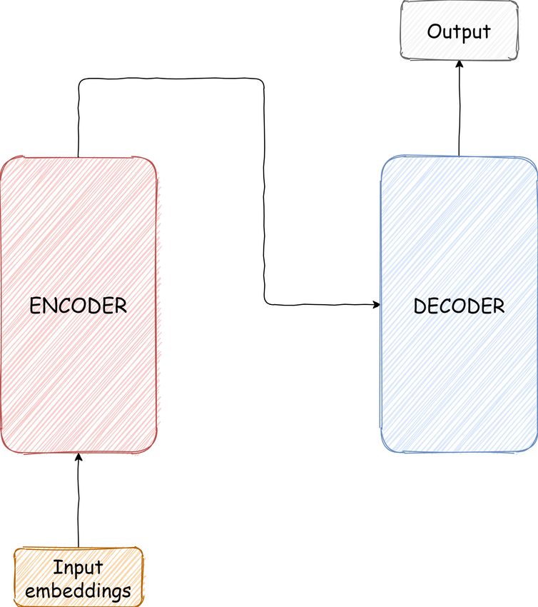
Contents

5 Preparing the experiments                                                             41
   5.1     Baseline models . . . . . . . . . . . . . . . . . . . . . . . . . . . . .    42
   5.2     Text-only transformers . . . . . . . . . . . . . . . . . . . . . . . . .     44
   5.3     Multimodal transformers . . . . . . . . . . . . . . . . . . . . . . . .      48
   5.4     Specifying the hypotheses . . . . . . . . . . . . . . . . . . . . . . .      49

6 Statistical analysis of experimental output data                                      52
   6.1     First exploratory plots . . . . . . . . . . . . . . . . . . . . . . . . .    52
   6.2     Testing the hypotheses . . . . . . . . . . . . . . . . . . . . . . . . .     61
           6.2.1   Hypothesis 1 . . . . . . . . . . . . . . . . . . . . . . . . . .     62
           6.2.2   Hypothesis 2 . . . . . . . . . . . . . . . . . . . . . . . . . .     68
           6.2.3   Hypothesis 3 . . . . . . . . . . . . . . . . . . . . . . . . . .     71
           6.2.4   Hypotheses 4 and 5 . . . . . . . . . . . . . . . . . . . . . . .     75
           6.2.5   Summary of hypothesis tests . . . . . . . . . . . . . . . . . .      77
   6.3     Some more findings . . . . . . . . . . . . . . . . . . . . . . . . . . .     78

7 Conclusion                                                                            80
   7.1     Summary . . . . . . . . . . . . . . . . . . . . . . . . . . . . . . . .      80
   7.2     Reflection . . . . . . . . . . . . . . . . . . . . . . . . . . . . . . . .   81
   7.3     Outlook . . . . . . . . . . . . . . . . . . . . . . . . . . . . . . . . .    82

References                                                                              84

                                            iv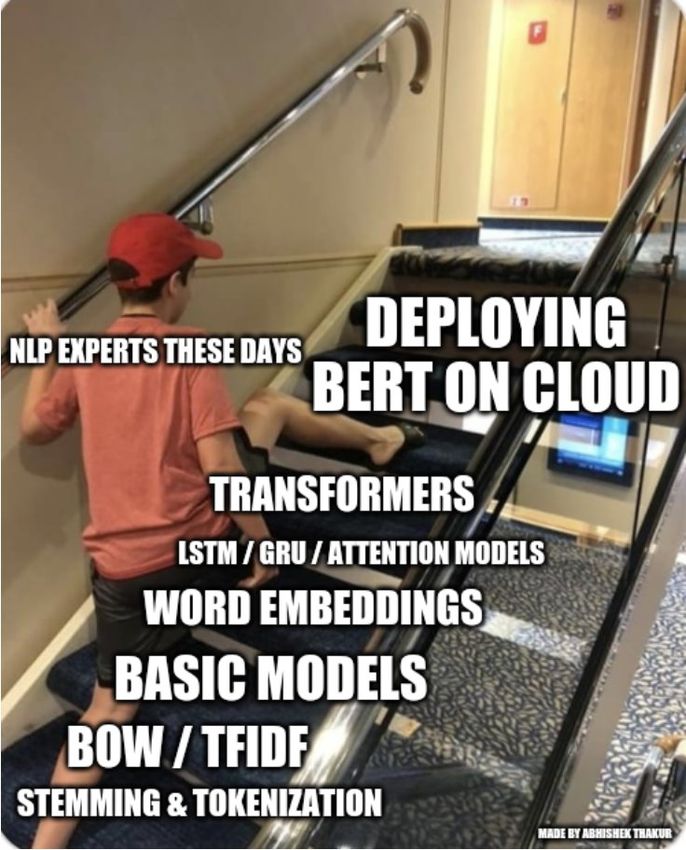
List of Figures
2.1 Distribution of ground truth labels - cooking data . . . . . . . . . . 8
2.2 Distribution of ground truth labels - voting data . . . . . . . . . . . 10
4.1 The BERT mountain. . . . . . . . . . . . . . . . . . . . . . . . . . . 24
4.2 Cheating your way up the BERT mountain. . . . . . . . . . . . . . 24
4.3 Illustration of transfer learning. . . . . . . . . . . . . . . . . . . . . 26
4.4 Cuncurrent training of BERT on MLM and NSP tasks. . . . . . . . 28
4.5 Sketch of encoder and decoder in a transformer. . . . . . . . . . . . 30
4.6 Bert not paying attention . . . . . . . . . . . . . . . . . . . . . . . 31
4.7 The transformer architecture. . . . . . . . . . . . . . . . . . . . . . 34
4.8 Multi-head attention with with eight words. . . . . . . . . . . . . . 36
4.9 Layer 4 and 12 from a pre-trained german BERT model. . . . . . . 38
5.1 Implemented baseline neural networks. . . . . . . . . . . . . . . . . 43
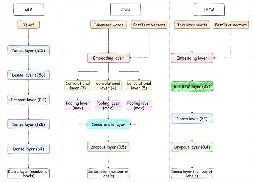
5.2 Workflow with the ‘multimodal-transformers‘ library. . . . . . . . . 49
6.1 Comparison of all experiments. . . . . . . . . . . . . . . . . . . . . 53
6.2 Comparison of all experiments over random states, model type, and
task. . . . . . . . . . . . . . . . . . . . . . . . . . . . . . . . . . . . 57
6.3 Comparison of all text-only transformer experiments by task. . . . . 59
6.4 Comparison of all text-only BERT, ConvBERT and DistilBERT. . . 60
6.5 Test setup for H1.1. . . . . . . . . . . . . . . . . . . . . . . . . . . . 63
6.6 Comparison between text-only and multimodal BERT models. . . . 65
6.7 Scatterplot comparing text-only and multimodal transformers. . . . 70
6.8 Comparison between transformer topologies. . . . . . . . . . . . . . 72
6.9 Comparison between text-only transformers and baseline models. . 76
v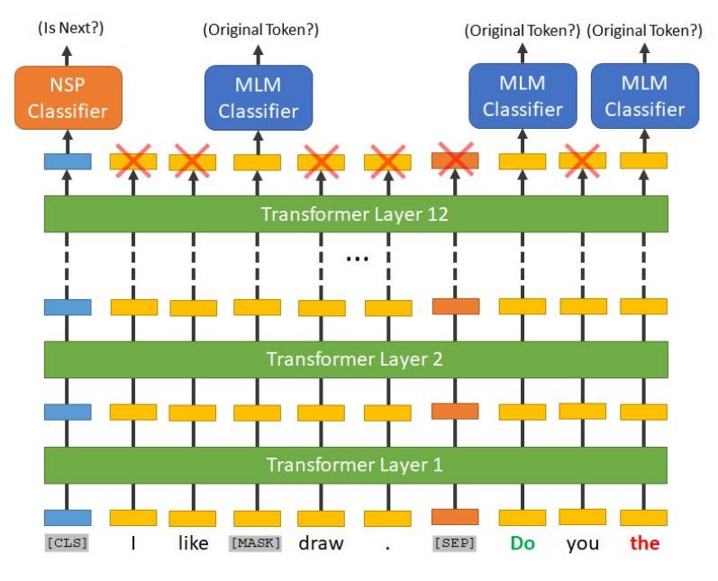
List of Tables

2.1   Comparison of data sources . . . . . . . . . . . . . . . . . . . . . .         4
2.2   Three rows from the cooking data . . . . . . . . . . . . . . . . . . .         6
2.3   Table of label explanations . . . . . . . . . . . . . . . . . . . . . . .      7
2.4   Three rows of Wandke annotations . . . . . . . . . . . . . . . . . .          13

3.1   Overview of conducted experiments . . . . . . . . . . . . . . . . . .         22

5.1   Sweeped RF and SVM hyperparameters. . . . . . . . . . . . . . . .             42
5.2   Overview of all pre-trained models used for experiments. . . . . . .          47

6.1   T-Test comparing differences between text-only and multimodal
      transformers - voting versus cooking task. . . . . . . . . . . . . . .        66
6.2   T-Test comparing differences between text-only and multimodal
      transformers - voting versus cooking task - version with both tasks
      binary. . . . . . . . . . . . . . . . . . . . . . . . . . . . . . . . . . .   67
6.3   T-Test comparing weighted F1 scores of text-only and multimodal
      transformers. . . . . . . . . . . . . . . . . . . . . . . . . . . . . . .     69
6.4   One-way ANOVA results for comparison between transformers. . . .              73
6.5   Tukey’s HSD Test for all possible pairwise comparisons of transformer
      topologies. . . . . . . . . . . . . . . . . . . . . . . . . . . . . . . . .   73
6.6   Tukey’s HSD Test for text-only versus baseline comparison. . . . . .          77

                                        vi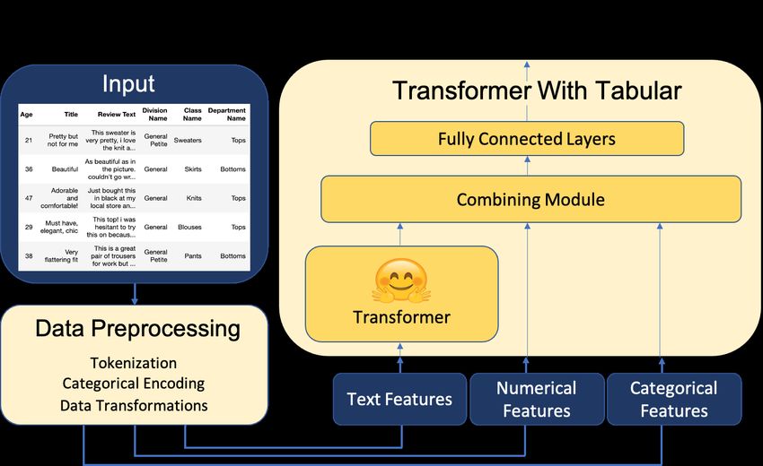
List of Abbreviations
ANOVA . . . . Analysis of variance
BERT . . . . . Bidirectional encoder representations from transformers
CPU . . . . . . Central processing unit
CV . . . . . . . Cross-validation
XLM . . . . . . Cross-lingual language models
ConvBERT . . Convolutional BERT
CNN . . . . . . Convolutional neural network
DistillBERT . Distilled BERT
Electra . . . .   Efficiently learning an encoder that classifies token replacements
                  accurately
FFN . . . . . . Feed-forward neural network
GAN . . . . . . Generative adversarial network
GPU . . . . . . Graphics processing unit
HSD . . . . . . Honestly significant difference
LSTM . . . . . Long short-term memory
ML . . . . . . . Machine learning
MLM . . . . .     Masked language modeling
MLP . . . . . . Multi-layer perceptron
NB . . . . . . . Naive bayes
NLP . . . . . . Natural language processing
NSP . . . . . . Next sentence prediction
NN . . . . . . . Neural network
OOV . . . . . . Out of vocabulary
RNN . . . . . . Recurrent neural network
Tf-idf . . . . . Term frequency–inverse document frequency
TN . . . . . . . Transformer network
YAML . . . . . Yaml ain’t markdown language

                                       vii
Transformers - from Bert to BERT
                                                                           1
In 2018, a dear childhood memory of many machine learners was being eradicated, or
at least replaced. Bert became BERT. The former is a yellow, likeable puppet with
a rather pessimistic attitude towards life. He and his friend Ernie live in Sesamstreet
with their friends, where they play funny and educational sketches for children.
   What on earth does this have to do with machine learning (ML)? Well, Bert, or
rather BERT, is also the acronym for Bidirectional Encoder Representations from
Transformers, which already sounds a lot more like ML. This is why my connotation
with Bert has changed recently; however, not necessarily for the worse. Bert was
a pleasant childhood memory. BERT is an exciting new technological advance in
the field of natural language processing (NLP). The risk of confusing them led to
quite a few memes on the internet. Much of this thesis will be about BERT and
the family of ML models it belongs to, the so-called transformers.
   BERT is the most widely known of these new deep neural networks. How these
transformer networks (TN) work and compare with other ML algorithms when
applied to NLP will be the topic of this thesis. This study aims to determine what
influence contextual features have on text classification in a dialogue setting and
a non-dialogue setting. To this end, different ML models will be compared, with
a particular focus on transformer networks. I will use two different NLP tasks.
The first concerns the cooking domain; the other is a political science task and
lies within voting. Both are classification tasks with short textual input as well

                                          1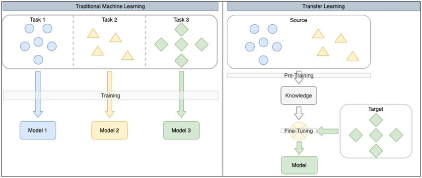
1. Transformers - from Bert to BERT

as some additional features. However, one data set comes from human dialogues.
The other is a collection of independent documents.
   Using TN for dialogue processing often uses only textual input as features. If
there are others, they are such that they can be computed on the fly during training
and classification. That is perfectly sensible since real-world systems have to be
operatable and it is very expansive to enrich user input with information annotated
by humans. However, if you could model human dialogue in a theoretically well-
founded way, and connect this with ML, it will likely increase performance. If the
increase is significant enough, realisations that are also feasible in practice will follow.
   Consider this the broader aim of the study. I try to evaluate whether the
theoretical model of a dialogue improves a TNs understanding of what a human
user wants. In this wake, I will also investigate how different TNs compare
with each other.
   There is comparably little literature on transformers yet, some two or three
textbooks on their application in NLP have been published at the time of this
writing. Papers are plentiful and the reader will see which matter for this thesis
soon. Most notably are Vaswani et al. (2017) and Devlin et al. (2019), were the
general idea of a TN and BERT were introduced. For theoretical considerations,
I will primarily refer to Wandke (2005). His approach will be used to bring the
notion of context into the data.
   There are many cognitive theories of human dialogue and researchers already
tried to integrate them with machine learning. (Malchanau 2019; Amanova et al.
2016) However, rather then only trying to get information about the human dialogue,
the annotations proposed in this thesis aim to enrich utterances with information
on the state of the conversational agent as well.
   After this introduction, I will start with preliminary remarks on my data, where
it comes from, and how it looks like. I explain the labels of both classification tasks
as well as textual and other input to the classifiers. In addition to that, there are
some theoretical explanations of the contextual features. In part three, I lay out my
research design by describing what rationale I will follow in the remainder of this
work. I also formulate my research question and hypotheses and give a first overview
of the ML experiments I made. Section four provides a methodological overview of
transformers and BERT. I will talk about transformers and their extension called

                                            2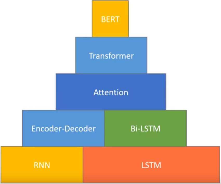
1. Transformers - from Bert to BERT

multimodal transformers because they are not yet widely known. There are concepts
like attention and transfer learning which deserve a more detailed discussion and
will also be covered in part four. For all the other classifiers, I refer the reader to
the relevant literature. After that, I will explain my concrete architectures and
classifier implementation in part five. Here, the hypotheses are also reformulated
and specified as to be strictly testable within this thesis’s framework. In part six, I
perform statistical analyses on all the experimental output data. I use inferential
statistical methods to evaluate model performance over 3720 experiments. The
last part concludes and gives an outlook.

                                          3
Preliminaries
2
2.1 Remarks on data - textual input feature and
labels
My data comes from two sources. The first one I will call cooking data from here
on, the second I will call voting data. They are from different domains and were
gathered in different contexts. Also, both pose different classification problems.
Still, they also share some characteristics.
Table 2.1: Comparison of data sources
Cooking data Voting data
Short textual input Short textual input
Whole sentences, incomplete sentences Whole sentences, word lists
2829 samples 2211 samples
Multi-label classification Binary classification
Gathered during an experiment Gathered during an opinion poll
Dialogue data, samples depend on each Each sample is an independent
other document
The most obvious difference, of course, are the domains from which each data set
comes. One is voting, and one is cooking. Why bring these two together?
The reason is that I have been trying to improve classification results on the
above-mentioned cooking corpus for a while when I attended a workshop where one
topic was NLP and its use for survey research. The presenters later also published
42. Preliminaries
a paper on how pre-trained models and transfer learning (we will see what that is
later in section 4.1.1) can help categorize survey respondents based on open-ended
questions. (Meidinger and Aßenmacher 2021) I found that I had a comparable
task with the cooking data. There are respondents who write whole sentences
in open-ended survey questions, and there are such people who give very short
replies - sometimes just a few words. This structure is comparable with the cooking
dialogue data. Sometimes there are very short utterances, grammatically not even
sentences, and sometimes there are whole, correct sentences. The difference is that
all the responses to be classified in the voting data are independent of each other
because they come from different people. In the cooking data, they are dialogues
and consequently not independent of each other.
Meidinger and Aßenmacher (2021) had good results with off the shelf transformer
models on their tasks. Therefore I want to bring these models into the domain
of dialogue data. To keep the comparison with a non-dialogue task, I decided to
include data from a study that I was part of and that was carried out during the
Bavarian state election of 2018. In the following section, I will briefly describe
both datasets and how they came to be.
Also, the text in both data sets is human-produced, so to say. The dialogue
data contains utterances as humans would speak them. The survey data - although
written - also contains such informal speech-like sentences while not being dialogical.
If you want to compare dialogue data with non-dialogue data, this is crucial. It
is hard to think about data of human utterances given as they would be spoken
and at the same time do not come from a dialogue.
2.1.1 Cooking data
The cooking data were gathered during experiments by Frummet et al. (2019). They
conducted in-situ experiments where a human assumed the role of a conversational
agent, like an Amazon Alexa. The idea was to simulate how a speech assistant with
human-like conversation abilities would interact with users. Subjects were given
cooking ingredients and then asked to cook a meal that they have not cooked before.
Experiments were done in users own kitchen at mealtime to make the situation
as realistic as possible. Therefore, users were also allowed to use ingredients they
had in store at home. However, the task still was to use as many of the provided
52. Preliminaries
ingredients as possible. To do so, they could ask their conversational agent (i.e. the
experimenter) anything. The agent then was allowed to look anything up on the
internet and respond to the best of his knowledge. From the whole textual material,
2829 user utterances were selected that were believed to hold a so-called information
need. “The term information need is often understood as an individual or group’s
desire to locate and obtain information to satisfy a conscious or unconscious need.”
(Wikipedia 2020; see also Rather 2018) In the cooking case, this could be the need
to get information about how much milk is needed at this step of the recipe. Three
rows of the data the experiments resulted in can be seen in table 2.2.
Table 2.2: Three rows from the cooking data
Label User utterance Reference Motiv and
goal
formation
Recipe Ähm kannst du mir Gerichte mit Spargel plan in
suchen mit möglichst vielen Milchprodukten.
Recipe Also ich hab überlegt Spargel mit plan in
Tomatenrühreiern dann wären drei Gerichte
weg ähm aber das passt glaub ich nicht
zusammen und keine Ahnung.
Recipe Ja oder äh hast du schon was gefunden? plan in
These are not all the features present in the cooking data, and the table is just
meant to give a first idea. Column three and four, for instance, are annotated
features that were coded according to the taxonomy, which I will describe later.
All 2829 user utterances are annotated with one of 13 information need labels.
These labels are Amount, Cooking technique, Equipment, Ingredient, Knowledge,
Meal, Miscellaneous, Preparation, Recipe, Temperature, Time, User Command,
and User Search Actions. Some of the names are telling, others not so much. In
the following table 2.3, you can see the explanations taken from the annotation
guidelines by Frummet (2019).
Just as Frummet et al. (2019) already found when looking into this corpus, I
find the labels’ distribution to be extremely skewed (see figure 2.1).
62. Preliminaries
Table 2.3: Table of label explanations
Label Explanation
Amount Amount related information needs occuring during
cooking.
Ingredient Ingredient related information needs occuring during
cooking.
Preparation Information needs that concretely relate to the
preparation process of a recipe that has been selected.
Cooking Information needs that relate to cooking techniques and
Technique preparation steps that aren’t specified in the selected
recipe.
Recipe Information needs relating to the recipe selection.
Time Information needs relating to temporal aspects of the
cooking/preparation process.
Equipment Information needs relating to the needed cooking
utensils.
Knowledge Information needs that relate to definitions of certain
aspects/entities occurring in the context of cooking.
Meal Information needs that relate to the currently prepared
meal. However, these are more general and do not
relate to certain preparation steps.
Temperature Information needs relating to temperature.
User Command Utterances of this class cannot be viewed as formal
information needs. They include commands users can
pose to the system.
User Search Utterances of this class cannot be viewed as formal
Actions information needs. They include search actions users
can pose to the system.
Miscellaneous Information needs that cannot be assigned to one of the
aforementioned classes.
This makes our cooking classification task even more challenging. Some labels
only have a dozen or even fewer samples, while Preparation has almost 800. The
three top classes easily account for half of all cases (i.e. samples). In section 3.3,
I will discuss what problems this causes and how they can be mitigated. The
utterances column of table 2.2 shows what participants said to the conversational
agent. This varies in length; the shortest utterances are one word long while
the longest one contains 95 words.
72. Preliminaries
Preparation
Ingredient
Amount
Cooking technique
Ground truth label
Recipe
Time
User Command
Knowledge
Miscellaneous
Equipment
Temperature
User Search Actions
Meal
0 200 400 600 800
Absolute count of label occurrence
Figure 2.1: Distribution of ground truth labels - cooking data
2.1.2 Voting data
The origin of this data set is a study carried out during the Bavarian state election of
2018. It was done by the chair of Political Science Research Methods in Regensburg.
Our team gathered data from over 16,000 voters and asked them open-ended as
well as closed questions. We surveyed people right after they came out of the voting
booth - a method called exit polls. A book with the results and exact methodology of
the study will be published in 2021, see Heinrich and Walter-Rogg (in appearance).
2211 of these roughly 16,000 repsondents replied to the open-ended questions
and will therefore be used in the remainder of this study. The wording of the
two open ended questions was the following:
Welches politische Thema hat Ihre Wahlentscheidung bei der heutigen
Landtagswahl am stärksten beeinflusst? (engl. Which political issue most
82. Preliminaries
influenced your voting decision in today’s state election? Translation
P.S.)
Falls Sie heute mit Ihrer Zweitstimme anders als bei der Landtagswahl
2013 gewählt haben: Können Sie uns bitte den wichtigsten Grund dafür
nennen? (engl. If you voted differently today with your second vote than
in the 2013 state election: Can you please tell us the most important
reason for this? Translation P.S.)
Both questions reflect issues that voters deem essential for making their decision.
In its extensive definition, a political issue can be anything that concerns voters.
It can be as broad as environmental politics and very specific, like when you can
mow your lawn at the weekends in certain constituencies. If it is high enough on
the political agenda and important to voters, the question of how society should
handle something becomes a political issue. (Schoen and Weins 2014, p. 285)
The labels in this task are binary. Either a person is a swing voter or not.1 I
coded this variable depending on whether a voter cast his second vote in the Bavarian
election of 2013 and 2018 for the same party. Just as in Germany’s general elections,
the Bavarian voting system lets its voters cast two votes. However, contrary to
the federal level, both - second and first vote - are equally important for the final
distribution of seats in parliament. (Bayerischer Landtag 2021) Three reasons made
me focus on second votes anyway. First, we did not ask for respondents first vote
in our study. Second, half of the voting population does not know the difference
between the second and first vote; this percentage has been stable for many years
(Westle and Tausendpfund 2019, p. 22) . Therefore, it is very likely that most
voters are note aware of the intricacies of the Bavarian state voting system either.
They will map the knowledge they have of the German system to the state level.
Third, the second vote is by definition the party vote, while the first vote is cast
1
Why did I opt for a binary problem here since labels in the cooking data have 13 different
classes? The reason is that generating all possible combinations of switch voting would lead
to a large number of labels. For instance, a person who voted CSU in 2013 has Greens, Social
Democrats, Free Voters, Alternative for Deutschland, and Free Democrats to choose from if they
intend to switch away from CSU. All in all, this leaves us with 30 labels (six parties make 6*5
combinations). Of course, I could concentrate on some exciting switch voting patterns, from CSU
to Greens, for examples; and choose 13 patterns that will be my labels. Then both tasks - voting
and cooking - would have the same number of labels. That, however, would eradicate a large
number of the switch voters from the 2211 samples, something that I can not reasonably do as
my data set is small enough already. Later, we will see that comparing binary and multi-label
classification tasks is an interesting setting and can deliver illuminating insights.
92. Preliminaries
Ground truth label
Swing voter
No swing voter
0 500 1000 1500
Absolute count of label occurrence
Figure 2.2: Distribution of ground truth labels - voting data
for a specific candidate. Therefore, we can justifiably assume that the difference in
the second vote is a good proxy for whether a voter switched parties or not. As
shown in figure 2.2, almost 1500 survey respondents are swing voters while only
about 700 are not swing voters. Therefore, the dataset also has unbalanced labels.
Still, this is nowhere near as dramatic as in the cooking data. It should also not
be a problem for the classifiers since both groups have sufficient samples.
2.2 Theoretical considerations and explanation
of additional features
2.2.1 Cooking data2
Human dialogue is dynamic and non-sequential. Understanding it as a succession
of exchanged utterances does resemble its complexity. (Malchanau 2019, p. ii) One
way to make this complexity accessible for ML algorithms would be to pass the
whole dialogue to a model and tell it which part of the dialogue you want to have
classified while still considering the whole dialogue. However, many ML models work
on a sample basis and can not digest a whole dialogue to do some classification.
Therefore, single utterances have to be put into the context of the dialogue rather
than the other way around. We annotated single samples with information on
dialogue context. How we did this will be explained now.
2
I took this subsection from a term paper that I wrote during a machine learning course at the
University of Regensburg. Course participants did the data coding as part of the final project.
102. Preliminaries
This section provides an overview of the schema based on which we annotated
additional features to the cooking data. The taxonomy we used was first proposed by
Wandke (2005), but the specific form applied here was derived from Henkel (2007);
there, it was employed in the context of human-computer interaction. The author
states that “this taxonomy, consisting of five dimensions, can be used to describe
a wide variety of assistance systems.” (Henkel 2007, p. 10, translation P.S.) This
is quite precisely what our coding aims to do. We want to annotate user requests
to the system, that is, queries that participants directed at the experimenter as
described in section 2.1. We identify at which stage of the taxonomy the system
currently is when it receives a particular request. This, in turn, helps to classify
user information needs correctly. A speech recognition system in the context of
cooking might then be better able to distil from the utterance the information it
needs to respond appropriately. This distillation, meaning categorization into one of
the 13 categories mentioned above, is what we aim at. Wandkes’ taxonomy has four
dimensions of which we only use one, the first. This first dimension has six phases
on which every utterance of experiment subjects was coded. Those phases are:
• Motive and goal formation
• Information intake
• Information analysis and integration
• Selection of an action
• Execution of an action
• Effects control.
The first phase, motive and goal formation, is present if a subject’s utterance
aims at receiving a justification or reason for an action. Looking for a specific
recipe also falls into this category. Two examples here are “But then why do I
only have to peel at the bottom?” or “Ok uh, I would like to cook something
and do not know what. What can I cook?”3
Phase two - information intake - applies when an utterance states a question
that aims at clarifying the state of the system or the state of the environment. “Can
3
All utterances were in the German language. I translated them here to make the text more
readable.
112. Preliminaries
you repeat that? I didn’t get that.” or “Because I still have some tomato sauce, I
just don’t know if there are pieces in it.” are two examples here.
The third phase of our taxonomy is called information integration. We code
an utterance as such whenever a subject has understood a response given by the
system but can not integrate it into the larger context of the situation (being the
task to cook a specific recipe). As two examples from our data, we can give “How
much Curcuma?” or “What is Cilantro?”.
We call phase four selection of an action. We annotate an utterance this way if
it concerns recipe selection and whenever a subject asks which option to choose from
two or more possibilities. In our data, “Um, I think I’ll have chickpea-lentil stew?”
and “Do I do this in a pot or with a kettle?” are both instances of this phase.
Our taxonomy’s penultimate category, called execution of an action, is pretty
much the logical consequence from phase four. When an action is selected, but
a subject still does not quite understand how to carry it out, we code it as
execution of an action. Two examples are “What does cooking mean?” and
“How does that work?”.
The last phase is called effects control and is used by subjects to assure themselves,
whether the execution of an action was correct. Often effects control occurs together
with the question about the next step. Here we can bring forward “I cut the onions,
what do I do now?” as an experiment participant’s exemplary statement.
One last codable dimension that is not part of Wandke’s taxonomy is reference.
It can be coded as either plan or activity. The former refers to the procedure of
the recipe/recipe selection. The latter is applied if an utterance concerns concrete
recipe steps and the execution of the recipe. A plan example would be “Um What
is the first step of the recipe?” An example of activity is “Does it say how many
uh teaspoons of vegetable broth you [need]?”
We hoped that the effort of coding all our data in this way would enrich it
enough to improve categorization substantially. Especially information on human
dialogue flow helps classification. Table 2.4 below shows some example utterances.
It also shows some columns we coded. Coding language was German. Some
words in the table are self-explaining. Fertig means done and offen means open
in englisch. When a phase has passed and the subject has proceeded, it is coded
122. Preliminaries
Table 2.4: Three rows of Wandke annotations
utterance reference motive i_intake i_integr select_act exec_act eff_cont
Welche Zutaten drin sind. Plan fertig in offen offen offen offen
Mach weiter. Plan fertig in offen offen offen offen
Bei welcher Plattform? Plan in offen offen offen offen offen
as done. The system’s current phase is coded as in, and everything that lies
ahead always receives the tag open.
Going into the details of the coding process is neither needed here nor within the
scope of this thesis. The interested reader can refer to me if coding schemes
should be made available.
In addition to those seen in table 2.4 there are seven more annotated features. I
will also include them in some experiments. They are
• previous information need,
• penultimate information need,
• need type,
• position of utterance in test person’s dialogue,
• step number,
• step component number,
• recipe number.4
The first two features are the two preceding labels of the current label to be classified.
That might raise some eyebrows since this essentially gives the classifiers much
information on the current ground truth label.5 However, since we are faced with a
dialogue task here, I wanted to model a ‘perfect world’, where I can capture the
cognitive task of engaging in a human conversation as best as possible. This is
known in the literature on dialogue state tracking, where lagged labels are often
4
Annotations for these features were done by Alexander Frummet.
5
To some extent, every annotation of data in a classification task gives information on the
ground truth. That is what annotating data then is about, helping the classifier by providing
additional information.
132. Preliminaries
employed to predict a system’s current state.6 (Jurafsky and Martin 2020, p. 509)
My reasoning here it that since we do not have a perfect human dialogue theory
yet, I opted to make sure my non-textual features will hold helpful information
for the classifier. After all, it is also possible that my additional features will
worsen results by adding a lot of noise.
Need type discerns information need queries into fact need, competence need,
and cooperation need. It is a rough presorting of the actual labels.
The position of an utterance in a test person’s dialogue is again relatively close
to the ground truth but is also a good proxy of modelling human conversation. In
cooking, it is quite evident that needs at the beginning are different from those
at the end of the process. In the beginning, I might wonder what I can cook
at all. In the end, this is, hopefully, not a question anymore. However, in most
practical applications, the length of the dialogue can not be known beforehand.
Therefore, this feature will not be available in such a fine-grained manner but
will be categorical in real-world applications.7
The last three mentions in the above bullet list, namely step number, step
component number, and recipe number, all hold information on the recipe that a
user is cooking. This, of course, also makes a difference in how the dialogue will
be unfolding. Talking about Viennese sausages with mustard is simple. Going
through a six-course menu for your wedding is a very different thing. Therefore
what you want to cook (i.e. the recipe) and how far you have come with it already
is very important for the classifier to know.
So much on the theoretical ideas behind and operationalizations of the annotated
features of the cooking data. The textual voting data have not been annotated
but rather come with additional features that were empirically surveyed in tandem
with the open-ended questions.
6
Of course, we do not want to predict the systems current state but rather the users information
need that the system may want to address.
7
What is still thinkable is when you have a huge amount of dialogue, you could calculate a
numerical state tracker feature. This can be done by estimating for a user query how far the query
is away from the average length of all dialogues. Such a value can then be above or below the
mean and would be a fine-grained global measure of how long the speech assistance process has
been going.
142. Preliminaries
2.2.2 Voting data
There are many reasons why a person might change his or her mind when choosing
which party to vote for. Things like party identification have proven a strong
predictor of individual voting behaviour over the last century. (Campbell et al.
1960) Nonetheless, it has been in decline for several decades. (Schoen 2014, p. 505)
Other factors like the candidates and specific, prevalent issues that change with
every election have considerably increased their explanatory power when we want
to explain how people vote. (Pappi 2003)
When predicting whether people will stay with the party they voted for the
last time, such variables (i.e. features) have usually been measured using surveys.
When faced with a classification task, social science and political science have long
resorted to logistic regression or the support vector machine (SVM). This might
have several reasons, one of which I think is that linear regression today is still
the uncontested workhorse of social science statistics. Any variety of it has an
easier time to become an accepted method within this discipline.8 That does not
mean that SVMs and others are not potent methods or that political science is
methodologically poor. Scientists made many great discoveries using regression.
It is nonetheless true that surveys usually have questions that we can not fully
harness by these methods, such as open-ended ones. However, these open-ended
questions often contain the most information on issues that voters are concerned
about. Moreover, if we believe that issue voting is on the rise, these questions and
the information they contain should be exploited more. Only very recently have
textual survey data and modern NLP methods been systematicly discovered for
voter classification. (Meidinger and Aßenmacher 2021) The focus here was for a
long time, and still is, data from social media.
I will use the survey data which I already described more closely in section
2.1.2. Some variables available in the data set are demographic. I include the
following additional features to improve the classification: age, education, and place
of residence. One more variable that is not demographic in nature is whether a
voter voted his or her way because of a candidate or a party. As a last amender to
8
Just as linear regression SVMs fit a line to a cloud of data points. Linear discriminant analysis
- also often used in social science - is a variety of linear regression. Its goal is comparable to that
of an SVM. (Backhaus et al. 2018, p. 204)
152. Preliminaries
the textual input, I bring in what party people voted for in the last two elections,
which at this point were the German federal election of 2017 and the Bavarian
state election of 2013.
This gives us the following as additional features:
• Age
• Education
• Place of residence9
• Vote for candidate or party
• Second vote at German general election 2017
• Second vote at Bavarian state election 2013
Stöss (1997, p. 56) finds that swing voters tend to be younger, and as people age,
they tend to stabilize their voting behaviour. This means that the information on
age could help classifiers to predict our target labels.
Research says swing voters tend to have comparatively high education. In my
case, the Bavarian state election, I also include the variable since I hope this variable
will help identify the large swath of people who voted for the Green Party the first
time. Green voters tend to be very well educated. This is uncontested in research
and literature. (Brenke and Kritikos 2020, p. 305; Stifel 2018, p. 176-177) My
hope is that the education variable will carry some information on swing voters
that opt for the Greens the first time.
Using the place of residence to classify voters goes as far back as to Lipset and
Rokkan (1967). Terms like the Worcester woman, the Holby City woman or the
Soccer Mum have been en vogue to describe voter profiles, especially in the United
Kingdom since the 2000s. (Spectator 2019; Aaronovitch 2009) What strikes is that
mostly these profiles describe some urban or suburban personas that policymakers
are especially keen to convince with their offers.10
9
Note that this is operationalized as the place where people went to cast their vote. However,
since they have to vote where they have their primary residence, this is very equivalent.
10
Of course, there are exceptions to this. The most prominent example here are presidential
elections in the United States of America, the last couple of which were decided in states like
Wisconsin, Illinois, or Michigan. Presidential candidates courted blue-collar workers, which do not
necessarily fit into the archetypal urban voter profile.
162. Preliminaries
The reasoning behind the last two variables is probably apparent. If people have
a steady party allegiance at least over the two previous elections, they might have
a lower chance of becoming swing voters in 2018. Therefore, these two variables
in unison can help separate swing voters from non-swing voters.
One more practical reason I chose all of these variables is that they are usually
included in most political science surveys that concern voting. If you can find a
reasonably good classifier using these variables, you can use it on pretty much
any larger survey conducted in the last decades. Furthermore, these are questions
that usually take no more than five minutes to get from people. Therefore, concise
surveys could also be used to amplify classifiers using social media data.11
We will now carry on with the research design where I quickly give an overview
of the conducted experiments. I will also layout how we go forward and formulate
my hypotheses.
11
Of course, this is delicate grounds. Not only ethically but also in the eyes of the public.
Classifying and predicting voter behaviour might seem an exciting scientific challenge, but from the
viewpoint of democratic theory, such techniques can be harmful. On microtargeting in Germany,
see for instance, Papakyriakopoulos et al. (2017).
17Research design
3
3.1 Research question
I will now describe how the design of the study is going to unfold. To this end, I
will first say a few words about the overarching research question and my general
discovery interest. In the second subsection of this part, I will formulate five
hypotheses to be investigated by experimentation in the latter half of this study.
Subsection three ends this part by sketching how I carried out my experiments.
I have already outlined my research interest in the introduction, but I want to
update it now as I already had the chance to give some background knowledge
to the reader. Generally speaking, I am concerned with two things here. First, I
want to find out how machine learning can improve dealing with human dialogue.
Second, I want to compare how transformers perform on classification tasks where
little data is available. A particular interest here is how they compare with each
other and with baseline models like LSTM or SVM.
What influence do additional numerical and categorical features have
in text classification tasks when using transformer models? Is there a
difference between dialogue data and non-dialogue data? How do different
transformer architectures compare with each other and with other ML
models in such circumstances?
This picks up on research by Vlasov et al. (2020) from a company called Rasa. Rasa
provides a backend for implementing chatbots using YAML (Yaml ain’t markdown
183. Research design
language) and markdown syntax. As the ML backbone of its software, Rasa also
uses a TN based architecture. Naturally, the company is primarily interested in
how these models perform on dialogue data. A chatbot is also very different from
the conversational agent, as it was simulated by the in-situ experiments I described
in section 2.1. Comparing transformers between dialogue tasks and non-dialogue
tasks as well as modelling the human-system interaction with the taxonomy from
section 2.2 is a new approach. It fills the gap of a more theory-driven use of
deep learning in dialogue processing.
3.2 Hypotheses formulation
I have already argued above (see section 2.1.1) on dialogue complexity. Of course,
this also means classification differs when there is no dialogue nature of the data at
all. This is the case with the voting data. Every sample is a single document and
unrelated to the other samples. Following my argumentation above, I postulate
that additional features will improve classification more when dialogue complexity
is negligible or even non-existent.1 This is so because we are not faced with
modelling the intricacies of human conversation but rather enrich our data with
more information. There is not much risk of messing up the signal that helps
the classifier predicting groups. Instead, we can be reasonably confident that the
information will be of help to the classifier.
H1: Using additional features to text-only classification tasks improves
classification better if documents are not dialogical and can be seen as
single atomic units.
What I also want to test is a less specific version of H1. Because there is
also the question of whether multimodal transformers, using additional features,
can improve classification at all. This is not self-evident for reasons other than
those elaborated around H1.2
H2: Multimodal transformers improve classification results compared
to text-only transformers.
1
For attempts to overcome the need to model complex dialogue flows, see Mrkšić et al. (2017).
2
There are also many technical pitfalls lurking here. One is, for instance, the question of
how to bring together (i.e. concatenate) text and non-text information. For a list of possible
concatenation methods in the multimodal-transformers library, see Georgian (2021).
193. Research design
As previously stated, I want to compare transformer performance within their
model family. The most pressing question here is whether the first TN that was
implemented in practice, namely BERT, gives the best results on my tasks; or is
it rather the case that any of the other new models like Electra or ConvBERT
yields the best scores? The hypothesis’s direction is hard to tell since these models
specifically boast about being applicable to any problem. Therefore, I leave it up
to empiricism to decide on this. Also, the literature and papers published on which
model is better can not be cited here, let alone summarised. A literature review
on this would probably a master’s thesis of its own. (for a real quick overview, see
Gillioz et al. 2020) However, it is mostly the case that new models, developed later,
claim to improve performance. This reasoning leads to H3.
H3: BERT, on average, delivers different classification results than
newer transformer architectures.
Then there is the almost obligatory comparison to classical baseline models.
In my case, they are split into deep learning and non-deep learning, leading
to H4 and H5.
H4: For small corpora, pre-trained transformer architectures deliver
better results on pure text classification than classical non-deep learning
models.
H5: For small corpora, pre-trained transformer architectures deliver
better results on pure text classification than non-attention-based deep
learning models.
Those are the five hypotheses that will guide us through the remainder of this
study. All of them only have the theory and data perspective so far. Therefore, I will
reformulate them more precisely in section 5.4. I will have had the chance then to
describe the experiments and their implementation more closely. With a background
on this, more measurable and precise hypotheses can be phrased. However, I also find
it essential to give some version of the hypotheses as early in the study as possible.
Also, given a broader version usually promotes comprehension. Therefore, I use this
two-step approach to hypotheses formulation. Of course, I do not want to make
any empirical postulation that is not strictly testable with my data or study setup.
203. Research design
3.3 Train-test split
With as little as about 2500 samples in each data set, choosing train and test
sets with intricate consideration is crucial. I opted against k-fold cross-validation
(CV) since this would reduce the number of sampels even further. Instead, I go for
stratified holdout validation, which I repeat ten times with ten randomly chosen
but constant random states. At this point, ML practitioners might become alert
since the changing of random states is always suspicious to them. In case of such
unbalanced labels (especially in the cooking data set), this was the only thing
advisable to do and can be seen as data augmentation. For instance, the cooking
test set contains 115 samples for one class and only seven for another. This is so
because these are also their relative proportions by which they occur in the overall
data. It is now crucial for the classification’s performance, whether a hard to classify
example made it into the test set or a relatively easy one was chosen. Therefore, I
conduct all my experiments with a fixed but randomly chosen set of random states
and average the results over these ten runs or report intervals. (López 2017; Han
2019) Furthermore, what one should not do with random states, is only trying to
optimize them. That not what I am trying to do. I am getting rid of the distorting
effect the random state has if such few samples are available.
3.4 Experiments overview
In total, I conducted 3720 experiments. Their split according to the different models
is shown in column six of table 3.1 below. I just want to give a quick overview
here before I go on. How I implemented the experiments, what libraries I used,
and so on will be the subject of the next part.
So for now, do not be bothered by how these architectures work or how exactly
they were implemented. We will come to that shortly. Even the meaning of
the acronyms in the first column is not essential for the moment. Note that all
experiments were done with both data sources (i.e. voting and cooking data) and
ten different random states as described in section 3.3.
21Introduction
Table 3.1: Overview of conducted experiments
Architecture Epochs Featurization n Additional n experi-
pre-trained features ments
models
NB NA Tf-idf NA No 20
SVM NA Tf-idf NA No 20
RF NA Tf-idf NA No 20
MLP 40 Tf-idf NA No 20
CNN 40 FastText NA No 20
LSTM 40 FastText NA No 20
BERT [1,2,3,4,5,6] BERT 9 Yes 1920
Tokenizer
DistilBERT [1,2,3,4,5,6] BERT 2 No 240
Tokenizer
ConvBERT [1,2,3,4,5,6] BERT 1 No 120
Tokenizer
Electra [1,2,3,4,5,6] Electra 7 No 840
Tokenizer
GPT2 [1,2,3,4,5,6] GPT2 2 No 240
Tokenizer
XLM [1,2,3,4,5,6] XLM Tokenizer 2 No 240
The second column shows the epochs that the models were trained for. This
only makes sense for the deep learning case, of course. The third column is the
number of different pre-trained models I iterated over with all experiments. The
number differs depending on how many pre-trained models are available online.
Mostly they are from a catalogue that comes with the Python library used in this
work. There, one can look up pre-trained models, more on this in section 5.2.
As shown in the fourth column, only pre-trained BERT models were available
from the multimodal-transformers library at the time of this writing. (Georgian
2021) Therefore, additional features are used only with pre-trained BERT ar-
chitecture models.
22Climbing the BERT mountain
4
BERT, a so-called transformer network, is a quite recent invention in NLP. To under-
stand how BERT in particular and a TN in general work will be the aim of this part.
In his YouTube series and book on BERT and transformers, ML teacher Chris
McCormick talks about learning and understanding these new models. He says
that they are usually taught to people who first came into contact with other
kinds of deep neural networks, namely convolutional neural network (CNNs) and
recurrent neural networks (RNNs). This, however, is not needed and might even
hinder an intuitive grasp of BERT. He calls this the BERT mountain, as shown
in figure 4.1. (McCormick 2020; McCormick 2019b)
Therefore, he explains BERT in a way that does not require any beforehand
understanding of other networks; where you do not have to climb the BERT
mountain. It is no small didactic problem if teachers have to presume or even build
sufficient knowledge before coming to the actual concept of interest. Since BERT and
transformers are quite different from other NLP networks, questioning the approach
of the BERT mountain is appropriate. There is also a wholly different view on the
BERT mountain that I find is very well summarized by the meme on the next page.
I do not think much interpretation is needed here. Understanding what came before
a groundbreaking invention like BERT is most likely essential to understanding the
invention itself. Both argumentations - the BERT mountain and its opposite - have
some validity. Unfortunately, I do not have space here to explain the fundamentals
234. Climbing the BERT mountain
Figure 4.1: The BERT mountain, from McCormick (2019a).
Figure 4.2: Cheating your way up the BERT mountain.
of ML and deep learning. I refer the reader to some great books covering everything
up to but not including transformers: Raschka and Mirjalili (2017), Aggarwal
(2018), Goldberg (2017), Kedia and Rasu (2020). I will therefore skip classifiers like
naive Bayes (NB), random forest (RF), support vector machine, CNN, and long
short-term memory (LSTM) networks. Also not explained here are the featurization
methods for textual data a will use later, namely term frequency-inverse document
frequency (tf-idf) and FastText. On FastText, see Joulin et al. (2016), Bojanowski
244. Climbing the BERT mountain
et al. (2017), and Kedia and Rasu (2020). It is a method for word vectorization
based on Word2Vec. (Mikolov et al. 2013) So basically, we skip the bottom third
of the BERT mountain seen in figure 4.1 and come straight to everything directly
related to BERT and transformers.
4.1 Transformer Networks - or what BERT is
Before I carry on, I quickly want to sketch what this subsection will be about.
Transformers are a relatively recent development in ML. A transformer makes
use of the concept of transfer learning, which is applying a model trained on a
different task and different data. There are various kinds of transfer learning, and
I will introduce them in the next section.
A transformer is composed of an encoder and a decoder. The encoder enriches
the input data and transforms it so that the decoder can perform a given task
on the data as good as possible. For instance, the decoder could enhance our
input word embeddings and the decoder would perform the actual classification.
Both encoder and decoder are composed of blocks which in turn are composed of
layers and sublayers. How many of these components are present in a transformer
varies. For example, the base version of BERT that we will use has 12 layers.
(Huggingface 2021a) I will soon describe in more detail how encoder and decoder
work in transformers.
Transfer learning and encoder-decoder layouts have not been new when trans-
formers came around. What has been quite a breakthrough is the invention of
attention by Bahdanau et al. (2016). Vaswani et al. (2017) then used this concept
in their paper Attention is all you need to propose its use in a neural network.
Attention is crucial to understanding transformers, and I will go to some length
explaining it in this subpart. For now, imagine it as giving the network the possibility
to determine which words in a sequence belong together and form meaning together
to produce a particular output. Especially bear in mind that this is theoretically
possible over arbitrarily long distances, meaning it does not matter how many
other words are between two words that belong together. This is an essential
part of human language that RNNs and CNNs have never fully mastered. In the
penultimate part of this section, we will dig deeper into attention.
In the final part of this section, I will walk through the vanilla transformer
network step by step.
254. Climbing the BERT mountain
4.1.1 The concepts of transfer learning and fine-tuning -
or how BERT is trained
Although the transformer and transfer learning sound quite similar, the latter has
not been invented with the former. Word2Vec, GloVe, FastText and other word
embeddings already do transfer learning. They train on one task and domain
and try to transfer the knowledge embedded in their vectors into other domains
and tasks. However, these embeddings are context-free. For instance, the word
bank could be the place where you deposit your money, or it could be the thing
you sit on in the park.
Figure 4.3: Illustration of transfer learning, from Bansal (2021, p. 106).
Bansal (2021) splits transfer learning into three main categories, two of which I deem
particularly relevant to understanding transformers. There is domain adaptation,
multi-task learning, and sequential learning. What he generally understands by
transfer learning can be seen in figure 4.3. While on the left side, we see traditional
ML models being built anew on every task and every data set, the right side shows
what happens if we incorporate transfer learning. We have a bigger data set that
we pre-train a model on. We then use that pre-trained model and the knowledge
incorporated within it to fine-tune the model for a new task and with new data.
The first, domain adaption is pretty much what machine learners do all the time.
They gather new data for their task. If you train a model by splitting up all your data
into train and test data and it performs well on the test data, that is a good starting
point. However, this test set still comes from the same data set. The ultimate
264. Climbing the BERT mountain
test would be to gather new data in different circumstances, for instance, take new
pictures of cats in different surroundings if the task were to spot cats in pictures.
Domain adaption will not be part of this research project. I do not have the time
or resources to gather new data from voters1 or conduct new cooking experiments.
The second kind of transfer learning, multi-task learning, is what BERT does.
If you wish to train a model that will perform reasonably well on a whole range
of tasks, you could train the model on all of these tasks. That would not leave
you with one but many different models. What was done instead when building
BERT was that BERT was trained on two specific tasks. Both of them do resemble
practical applications to some degree, but they are not what you would come up
with when trying to get the best model for a specific task.
The first task BERT was given - called masked language modelling (MLM) -
goes like this: In every input sentence, a fraction of all words get masked, meaning
BERT does not know anymore which word it is receiving as input. Another fraction
gets randomly replaced by a random token from the vocabulary and the remainder
of input words stays untouched. The aim is to train BERT to correctly learn the
masked and swapped tokens to output the correct original sentence, although the
input has been severely mutilated. (Kedia and Rasu 2020, p. 277)
The second task - next sentence prediction (NSP) - feeds BERT with pairs of
text passages. Fifty per cent of the time, the latter passage truly belongs to the
former. In other examples, the second text passage is just a randomly selected
text from the whole data set. The aim of BERT here is straightforward. Do
these two text passages actually belong to each other? Should the second follow
the first? (Kedia and Rasu 2020, p. 278)
As can be seen in figure 4.4, in practice, BERT has to solve both tasks
simultaneously. The combination of both is something that I think is quite hard
to find a real-world application for. Maybe some intelligence service could be
faced with very distorted documents that might resemble this task that BERT
1
What I could do is taking the gargantuan amount of political survey data gathered in the
past 100 years or so. Many of them ask the questions we were asking in our survey, and many
of them include the demographic variables I use for my models in the latter part of this thesis.
Bringing all this data together would still be a massive project in and of itself. One recent paper
by Meidinger and Aßenmacher (2021) does something like this with survey data from the United
States. They show how open-ended survey questions and pre-trained transformers can help to
learn about peoples political attitudes.
27You can also read