A comprehensive in situ and remote sensing data set from the Arctic CLoud Observations Using airborne measurements during polar Day (ACLOUD) ...
←
→
Page content transcription
If your browser does not render page correctly, please read the page content below
Earth Syst. Sci. Data, 11, 1853–1881, 2019
https://doi.org/10.5194/essd-11-1853-2019
© Author(s) 2019. This work is distributed under
the Creative Commons Attribution 4.0 License.

          A comprehensive in situ and remote sensing data set
           from the Arctic CLoud Observations Using airborne
          measurements during polar Day (ACLOUD) campaign
           André Ehrlich1 , Manfred Wendisch1 , Christof Lüpkes2 , Matthias Buschmann3 , Heiko Bozem4 ,
           Dmitri Chechin2 , Hans-Christian Clemen5 , Régis Dupuy6 , Olliver Eppers4,5 , Jörg Hartmann2 ,
                Andreas Herber2 , Evelyn Jäkel1 , Emma Järvinen7 , Olivier Jourdan6 , Udo Kästner8 ,
           Leif-Leonard Kliesch9 , Franziska Köllner6 , Mario Mech9 , Stephan Mertes8 , Roland Neuber10 ,
        Elena Ruiz-Donoso1 , Martin Schnaiter11 , Johannes Schneider6 , Johannes Stapf1 , and Marco Zanatta2
                     1 Leipziger       Institut für Meteorologie (LIM), Universität Leipzig, Leipzig, Germany
       2 Alfred-Wegener-Institut,       Helmholtz-Zentrum für Polar- und Meeresforschung (AWI), Bremerhaven, Germany
                               3 Institut für Umweltphysik (IUP), Universität Bremen, Bremen, Germany
                  4 Institut für Physik der Atmosphäre (IPA), Johannes Gutenberg-Universität, Mainz, Germany
                   5 Particle Chemistry Department, Max-Planck-Institut für Chemie (MPIC), Mainz, Germany
                6 Laboratoire de Météorologie Physique (LaMP), Université Clermont Auvergne/OPGC/CNRS,

                                                   UMR 6016, Clermont-Ferrand, France
                                7 National Center for Atmospheric Research (NCAR), Boulder, CO, USA
                              8 Leibniz-Institut für Troposphärenforschung (TROPOS), Leipzig, Germany
                     9 Institut für Geophysik und Meteorologie (IGM), Universität zu Köln, Cologne, Germany
         10 Alfred-Wegener-Institut, Helmholtz-Zentrum für Polar- und Meeresforschung (AWI), Potsdam, Germany
      11 Institut für Meteorologie und Klimaforschung, Karlsruher Institut für Technologie (KIT), Karlsruhe, Germany

                                Correspondence: André Ehrlich (a.ehrlich@uni-leipzig.de)

                                    Received: 8 June 2019 – Discussion started: 14 June 2019
                      Revised: 29 October 2019 – Accepted: 30 October 2019 – Published: 29 November 2019

      Abstract. The Arctic CLoud Observations Using airborne measurements during polar Day (ACLOUD) cam-
      paign was carried out north-west of Svalbard (Norway) between 23 May and 6 June 2017. The objective of
      ACLOUD was to study Arctic boundary layer and mid-level clouds and their role in Arctic amplification. Two
      research aircraft (Polar 5 and 6) jointly performed 22 research flights over the transition zone between open
      ocean and closed sea ice. Both aircraft were equipped with identical instrumentation for measurements of basic
      meteorological parameters, as well as for turbulent and radiative energy fluxes. In addition, on Polar 5 active
      and passive remote sensing instruments were installed, while Polar 6 operated in situ instruments to characterize
      cloud and aerosol particles as well as trace gases. A detailed overview of the specifications, data processing,
      and data quality is provided here. It is shown that the scientific analysis of the ACLOUD data benefits from the
      coordinated operation of both aircraft. By combining the cloud remote sensing techniques operated on Polar 5,
      the synergy of multi-instrument cloud retrieval is illustrated. The remote sensing methods were validated us-
      ing truly collocated in situ and remote sensing observations. The data of identical instruments operated on both
      aircraft were merged to extend the spatial coverage of mean atmospheric quantities and turbulent and radiative
      flux measurement. Therefore, the data set of the ACLOUD campaign provides comprehensive in situ and remote
      sensing observations characterizing the cloudy Arctic atmosphere. All processed, calibrated, and validated data
      are published in the World Data Center PANGAEA as instrument-separated data subsets (Ehrlich et al., 2019b,
      https://doi.org/10.1594/PANGAEA.902603).

Published by Copernicus Publications.
1854                                                                                     A. Ehrlich et al.: The ACLOUD data set

1   Introduction                                                    aircraft is provided. The aim is to document the campaign-
                                                                    specific instrument operation, data processing, uncertainties
                                                                    of the derived quantities, and data availability to facilitate a
The considerable increase in Arctic near-surface tempera-           widespread use of the data in a broad field of scientific analy-
tures within the last 3 to 4 decades, a phenomenon commonly         sis. To understand the aim and flight patterns of each research
called Arctic amplification (Serreze and Barry, 2011), sig-         flight, in Sect. 2 an overview of the main scientific targets and
nificantly exceeds the global warming and is associated with        the most common flight patterns is provided. The instrumen-
the decrease in Arctic sea ice. To improve the understand-          tation, calibration, and data processing of measurements on
ing and the ability to predict these changes, several interna-      Polar 5 and 6 are described in Sects. 3 and 4. Due to the op-
tional efforts, including joint model evaluations such as the       eration of two identical aircraft (partly with identical instru-
Year of Polar Prediction within the Polar Prediction Project        mentation), several benefits arise for the data analysis. Coor-
(Jung et al., 2016) and a series of observational field cam-        dinated observations from both aircraft flying in close collo-
paigns are underway. These observations obtained by land-           cation, e.g. remote sensing and in situ measurements, were
based (Uttal et al., 2016), ship-based, and airborne activities     combined as demonstrated in Sect. 5.1. In Sect. 5.2, the con-
(Wendisch et al., 2019) are essential to identify the dominant      sistency of data from similar instruments operated on both
atmospheric processes and provide an observational basis for        aircraft is validated, which allows for merging observations
model and satellite data validations. Due to the diversity of       from both aircraft into a single data set. The data availability,
instrumentation and required measurement strategies, these          including links to the published data sets, is given in Sect. 6.
field campaigns often target specific components of the Arc-
tic climate system.
   In May and June 2017, two concerted field studies, the
                                                                    2    Scientific targets of the research flights
Arctic CLoud Observations Using airborne measurements
during polar Day (ACLOUD) campaign and the Physical
                                                                    The ACLOUD aircraft campaign performed 22 research
Feedbacks of Arctic Boundary Layer, Sea Ice, Cloud and
                                                                    flights between 23 May and 26 June 2017, which are listed
Aerosol (PASCAL) ship cruise were performed to improve
                                                                    in Table 1 (flight numbers start with no. 4, neglecting the
our understanding of the role of clouds and aerosol particles
                                                                    test and ferry flight nos. 1–3). In total, measurements were
in Arctic amplification (Wendisch et al., 2019). Both cam-
                                                                    obtained in 165 flight hours distributed equally to both air-
paigns were conducted within the framework of the “Arc-
                                                                    craft. A joint operation of Polar 5 and 6 was coordinated
tic Amplification: Climate Relevant Atmospheric and Sur-
                                                                    for 16 research flights. The general scientific goals of all
face Processes, and Feedback Mechanisms (AC)3 ” project
                                                                    ACLOUD flights are summarized by Wendisch et al. (2019).
(Wendisch et al., 2017). During ACLOUD, two research air-
                                                                    Most flights included different flight sections to address more
craft, Polar 5 and Polar 6 (Wesche et al., 2016), were oper-
                                                                    than only one of the specific objectives. The dedicated mis-
ated, which were stationed on Svalbard (Longyearbyen, Nor-
                                                                    sions and flight patterns can be categorized as follows.
way). For PASCAL the Research Vessel (R/V) Polarstern
(Knust, 2017) entered the sea ice north of Svalbard, where
an ice floe camp (including a tethered balloon, ground-                 – Characterization of boundary layer clouds by remote
based remote sensing, and in situ sampling of aerosol par-                sensing and in situ microphysical measurements. For
ticles) was set up for 2 weeks (Macke and Flores, 2018).                  this objective, 11 closely collocated flights with Polar
These observations were accompanied by permanent mea-                     5 performing remote sensing in high altitudes (up to
surements at the joint research base AWIPEV at Ny-Ålesund                 4000 m) and Polar 6 sampling clouds below (down to
on Svalbard (Neuber, 2006) operated by the Alfred Wegener                 70 m above sea level) were conducted (column “col-
Institute (AWI) and the French Polar Institute Paul-Émile                 located” in Table 1). The collocation of both aircraft
Victor (IPEV; AWIPEV). The airborne operations during                     aims to study the identical cloud section without hor-
ACLOUD were coordinated with the ship-based (PASCAL)                      izontal or temporal mismatch. To obtain vertical pro-
and ground-based activities (AWIPEV) and focused on the                   files of cloud and aerosol particle properties and trace
area north-west of Svalbard, linking the observations at AW-              gases, horizontal legs in different altitudes were flown in
IPEV and on Polarstern.                                                   double-triangle pattern, where Polar 6 changed altitude
   The general objectives of ACLOUD and PASCAL, the op-                   after each triangle and Polar 5 remained at high altitude.
erated instrumentation, a summary of the measurement activ-               Longer straight flight sections crossing the marginal
ities, and first highlights of the data analysis are presented by         sea ice zone aim to study the contrast of clouds over
Wendisch et al. (2019), while the meteorological conditions               open ocean and sea ice and release series of dropson-
during the observational period were analysed by Knudsen                  des. Table 1 indicates which flights include segments
et al. (2018). In this paper, a detailed overview of the pro-             with cloud remote sensing (CRS) and in situ cloud and
cessed ACLOUD data set obtained on board both research                    aerosol particle and trace gas measurements (in situ).

Earth Syst. Sci. Data, 11, 1853–1881, 2019                                           www.earth-syst-sci-data.net/11/1853/2019/
A. Ehrlich et al.: The ACLOUD data set                                                                                                   1855

Table 1. Overview of ACLOUD flights, including the takeoff and landing times of Polar 5 and 6 and the general scientific target of the flight.
The objectives are categorized into cloud remote sensing (CRS), in situ cloud and aerosol particle and trace gas measurements (in situ),
surface fluxes (SF), and flux profiles (FP). The remaining columns indicate if Polar 5 and 6 overflew Polarstern (PS) or Ny-Ålesund (NÅ),
flew in collocated formation (Polar 5 above Polar 6), or were coordinated with an overpass of the NASA A-Train constellation.

   No.    Date in      Takeoff–landing (UTC)                    Scientific target             Collocated     Polarstern (PS) /    A-Train
          2017       Polar 5         Polar 6         CRS      In situ   SF    FP                             Ny-Ålesund (NÅ)
   4      23 May     09:12–14:25     –               CRS               SF
   5      25 May     08:18–12:46     –               CRS
   6      27 May     07:58–11:26     –               CRS                                                                             X
   7      27 May     13:05–16:23     13:02–16:27     CRS                                           X
   8      29 May     04:54–07:51     05:11–09:17     CRS                      FP
   9      30 May     –               09:18–13:30     Vertical mapping of aerosol particles                   PS
   10     31 May     15:05–18:57     14:59–19:03     CRS In situ SF                                          PS
   11     2 June     08:13–13:55     08:27–14:09     CRS In situ                                   X         PS, NÅ                  X
   12     4 June     –               10:06–15:39             In situ                                         PS                      X
   13     5 June     10:48–14:59     10:43–14:44     CRS In situ SF                                X         PS
   14     8 June     07:36–12:51     07:30–13:20     CRS In situ SF FP                             X         PS, NÅ                  X
   15     9 June     08:00–09:21     07:56–09:18        P5/P6 instrument comparison                X
   16     13 June    14:56–16:55     14:57–17:16               P5/P6 calibration                   X
   17     14 June    12:48–18:50     12:54–17:37     CRS In situ              FP                   X         PS
   18     16 June    04:45–10:01     04:40–10:31     CRS In situ                                             PS                      X
   19     17 June    09:55–15:25     10:10–15:55     CRS In situ              FP                   X
   20     18 June    12:03–17:55     12:25–17:50     CRS In situ              FP                   X         PS
   21     20 June    07:30–13:55     07:37–13:27     CRS In situ SF FP                                       PS
   22     23 June    10:57–14:39     10:37–14:52             In situ                               X         NÅ
   23     25 June    11:09–17:11     11:03–16:56                       SF FP
   24     26 June    –               08:33–10:39                 P6 calibration
   25     26 June    12:34–15:17     12:32–14:48                       SF FP                       X

  – Satellite validation. Five research flights contain legs,                – Profiles of turbulent and radiative fluxes. Eight flights
    which are time synchronized with overpasses of the                         were partly dedicated to characterizing the vertical pro-
    NASA A-Train satellite constellation (Stephens et al.,                     files of turbulent and radiative fluxes in the cloud-free
    2018, column “A-Train”) and flown parallel to their                        and cloudy atmospheric boundary layer (column “FP”).
    tracks. Within a certain time window, which depends                        For this mission, vertical stacks of short horizontal legs
    on wind speed and cloud evolution, these data aim for                      in different altitudes were flown across the main wind
    a direct comparison of cloud structures observed from                      direction. During three flights, these patterns were flown
    satellite and aircraft.                                                    jointly by both, horizontally separated from each other
                                                                               by 20–50 km.
  – Comparison with ground-based observation. When
    possible, flight activities were coordinated with the                    – Vertical mapping of aerosol particles. One single flight
    PASCAL campaign of the research vessel Polarstern,                         of Polar 6 aimed to map the vertical distribution of
    which was met 10 times (column “Polarstern”), and                          aerosol particles at two locations along the main wind
    with ground-based observations at Ny-Ålesund (column                       direction. To do so, at each location horizontal legs in
    “Ny-Ålesund”), which was overpassed 4 times. To com-                       different altitudes were flown across the wind direction.
    pare the ground-based and airborne observations in an                    – Instrument calibration and comparison. Three flights
    area of comparable size, mostly double-triangle patterns                   were dedicated to comparing the measurements of both
    were performed over the ground stations.                                   aircraft and calibrating different instruments. For the
                                                                               comparison a joint ascent with both aircraft separated
  – Near-surface turbulent and radiative fluxes. To quan-                      by less than 100 m was flown. The calibrations required
    tify the turbulent and radiative fluxes at the surface (col-               instrument-specific calibration flight patterns.
    umn “SF” in Table 1), long horizontal flight segments at
    low altitude were implemented in the research flights. In               For each flight, a flight report was compiled summarizing
    the case of cloudy conditions, a flight altitude below the           the major information about the flight required to recapture
    cloud base was chosen.                                               the objectives and their implementation. The flight reports

www.earth-syst-sci-data.net/11/1853/2019/                                                 Earth Syst. Sci. Data, 11, 1853–1881, 2019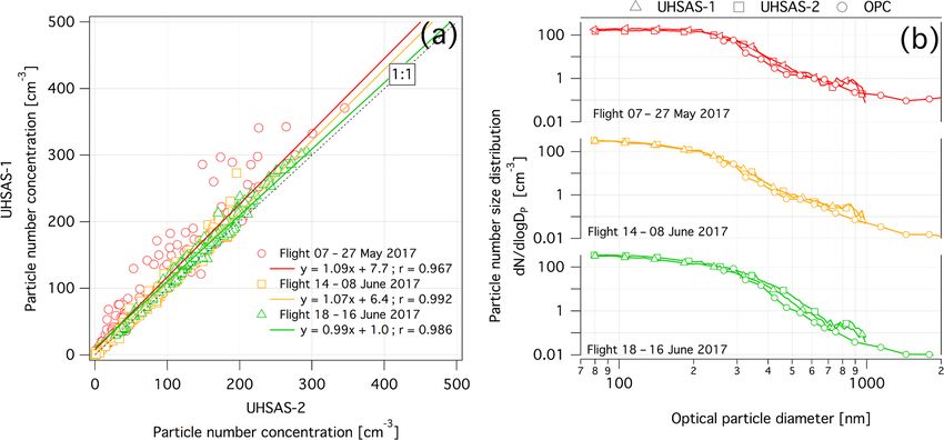
1856                                                                                    A. Ehrlich et al.: The ACLOUD data set

are provided in the Supplement. Coordinated flights of Po-          were merged by complementary filtering at a frequency of
lar 5 and Polar 6 are combined in a single report. The reports      0.1 Hz.
include the flight track, description of predicted and present         The wind vector was calculated by applying the procedure
weather conditions, instrument performance, photographs,            described by Hartmann et al. (2018). The method consid-
and notes.                                                          ers a careful calibration of the initial wind measurements,
                                                                    which is based on a combination of the differential mea-
                                                                    surement capabilities of the GPS and the high-accuracy INS.
3     Instrumentation on Polar 5                                    With the precise aircraft position and attitude, the horizontal
                                                                    wind components are derived with an absolute accuracy of
A comprehensive general overview of airborne instrumenta-           0.2 m s−1 for straight and level flight sections. The vertical
tion in general is given by Wendisch and Brenguier (2013).          wind can only be analysed as the deviation from the average
Many of the instruments installed on Polar 5 and 6 are de-          vertical wind. To do so, the mean wind vector was averaged
scribed in detail in this reference. Polar 5 was primarily op-      for flight sections of at least several kilometres length. For
erated as a remote sensing aircraft. Active radar and lidar ob-     straight and level flight sections, the accuracy of the vertical
servations were combined with passive spectral solar and mi-        wind speed relative to the average is about 0.05 m s−1 .
crowave sensors, including an imaging spectrometer, a fish-            The temperature measurements were corrected for the adi-
eye camera, a microwave radiometer, and a Sun photome-              abatic heating of the air by the dynamic pressure. The ab-
ter. For measurements of turbulent and radiative energy flux        solute accuracy of the temperature measurements is 0.3 K
densities, a nose boom and broadband solar and terrestrial          with a resolution of 0.05 K. The lateral displacement be-
radiation sensors (pyranometer and pyrgeometer) were in-            tween wind and temperature sensors (radial distance to the
stalled. Profiles of meteorological parameters were collected       centre of the five-hole probe of 16 cm and an axial dis-
by dropsondes. The instrumentation is listed in Table 2.            tance of 35 cm) was found to be not critical. For typical true
                                                                    air speeds of 60 m s−1 , this axial distance corresponds to a
3.1    High-frequency wind vector, air temperature, and             time lag of about 6 × 10⁻³ s, which is less than one sam-
       humidity                                                     ple at the recording frequency. Additionally, Polar 5 nose
                                                                    boom carried a closed-path LI-7200 gas analyser for CO2
On both aircraft, identical sensors were installed in a nose        and H2 O concentration measurements. The performance of
boom for high-frequency measurements of the wind vector             the analyser with respect to airborne humidity flux mea-
and the air temperature (Hartmann et al., 2018). The basic          surements has been tested, as described in detail by Lam-
sensors are an Aventech five-hole probe placed at the tip of        pert et al. (2018). For slow humidity measurements (fre-
the nose boom and an open-wire Pt100 installed sidewards in         quency of 1 Hz), a Vaisala HMT-333, which includes a tem-
a Rosemount housing. All data were recorded and published           perature and HUMICAP humidity sensor, was mounted in
with a frequency of 100 Hz (Hartmann et al., 2019a, https:          a Rosemount housing. Based on the temperature measure-
//doi.org/10.1594/PANGAEA.900880). The response time of             ments (uncertainty of 0.1 K), the humidity data were cor-
the sensors is below 0.01 s, well suited for atmospheric tur-       rected for adiabatic heating and reach an accuracy of 0.4 %
bulence flux measurements (Lee, 1993). The five-hole probe          (Hartmann et al., 2018). These measurements were merged
is heated during the flight to prevent icing. It is equipped with   into a reduced 1 Hz basic meteorological data set providing
a purging system to eject water that might have entered the         aircraft position, air pressure, temperature, relative humid-
central hole. Thus, measurements within clouds are reliable.        ity, and the horizontal wind vector (Hartmann et al., 2019b,
   Pressure measurements in the five-hole probe are recorded        https://doi.org/10.1594/PANGAEA.902849).
by differential pressure transducers of type Setra 239 R for           The achieved accuracy and temporal resolution of wind
angle of attack, angle of sideslip and the dynamic pressure         and temperature measurements are sufficient to derive tur-
and by a Setra 278 for the static pressure. To convert the wind     bulent fluxes of momentum and sensible heat in the atmo-
vector measured with respect to the aircraft frame into Earth-      spheric boundary layer with the eddy-covariance method
fixed coordinates, the position, movement, and attitude of the      (e.g. Busch, 1973). When using the 100 Hz data delivered to
aircraft is measured with a combination of a high-precision         PANGAEA, note that the calibration of the five-hole probe
global positioning system (GPS) receiver and an inertial nav-       is only valid for straight and level flights. The majority of
igation system (INS). The INS, a Honeywell Laseref V, pro-          measurements during ACLOUD were obtained over sea ice
vides longitude, latitude, ground speed, and angular rates          in slightly unstable or stable stratification where turbulent
and calculates the pitch, roll, and true heading angles with        heat fluxes are rather small (heat fluxes in the order of a few
an accuracy of 0.1◦ (roll and pitch) and 0.4◦ (true heading).       W m−2 ). Such low flux conditions represent a challenge to
A Novatel GPS FlexPak6 receiver supports the calculation            instrumentation and measurement strategy and lead to less
of the position and the velocity vector. Doppler-derived ve-        relative accuracy compared to turbulent fluxes derived in
locities (“Novatel bestvel”) are obtained with a precision of       strong convective condition as, for example, cold air out-
0.03 m s−1 . For the final data product, the INS and GPS data       breaks.

Earth Syst. Sci. Data, 11, 1853–1881, 2019                                          www.earth-syst-sci-data.net/11/1853/2019/
A. Ehrlich et al.: The ACLOUD data set                                                                                               1857

Table 2. Overview of the instrumentation of Polar 5 and 6 and the measured quantities that are part of the database. λ is wavelength, ν is
frequency, T is temperature, and p is atmospheric pressure. RH is relative humidity, FOV is field of view, PNSD is the particle number size
distribution, rBC is refractory black, and Dp is the particle diameter.

      Aircraft     Instrument             Measured quantities, range, and sampling frequency
      Meteorology
      P5           Dropsondes (RS904)     Profiles of T , p, RH, horizontal wind vector, 1 Hz
      Turbulence
      P5&P6        Nose boom sensors      T , p, wind vector, 100 Hz
      Radiation
      P5&P6        CMP-22 pyranometer     Solar irradiance (upward, downward, broadband λ = 0.2–3.6 µm), 20 Hz
      P5&P6        CGR-4 pyrgeometer      Terrestrial irradiance (upward, downward, broadband λ = 4.5–42.0 µm), 20 Hz
      P5&P6        KT-19                  Brightness temperature (upward nadir, λ = 9.6–11.5 µm), 20 Hz
      Remote sensing
      P5           SMART Albedometer      Spectral irradiance (upward, downward λ = 400–2155 nm), 2 Hz
                                          Spectral radiance (upward, FOV = 2.1◦ , λ = 400–2155 nm), 2 Hz
      P5           AISA Eagle/Hawk        Spectral radiance (upward, swath = 36◦ , λ = 400–2500 nm), 20–30 Hz
      P5           180◦ fisheye camera    Spectral radiance (lower hemisphere, RGB channels), 6 s
      P5           AMALi                  Particle backscattering coefficient (λ = 355, 532 nm), cloud top height,
                                          particle depolarization (λ = 532 nm), 5 s
      P5           MiRAC-A                Radar reflectivity factor, Doppler spectra, ν = 94 GHz, tilted by 25◦ , 1–2 s
                                          brightness temperature (BT), ν = 89 GHz, tilted by 25◦ , 1–2 s
      P5           MiRAC-P                Brightness temperature (BT), ν = 183.31, 243, 340 GHz, nadir view, 1–2 s
      P5           Sun photometer         Spectral aerosol optical depth (AOD) λ = 400–2000 nm), 1 s
      Aerosol microphysics
      P6           CPC                    Number concentration, Dp = 10 nm–3 µm, 3 s
      P6           PSAP                   Absorption coefficient, λ = 565 nm), 30 s
      P6           SP2                    rBC mass and number concentration, PNSD, rBC mass: 0.26–125 fg, Dp = 65–510 nm, 1 s
      P6           UHSAS-1                Aerosol PNSD, Dp = 60 nm–1 µm, 3 s
      P6           UHSAS-2                Aerosol PNSD, Dp = 80 nm–1 µm, 1 s
      P6           Grimm Sky-OPC          Aerosol PNSD, Dp = 250 nm–5 µm, 6 s
      Cloud microphysics
      P6           PHIPS                  Angular scattering function, particle shape, Dp = 20–700 µm, 20 Hz
      P6           SID-3                  Cloud PNSD, particle shape, sub-micrometre scale complexity, Dp = 5–45 µm, 1 Hz
      P6           CDP-2                  Cloud PNSD, Dp = 2–50 µm, 1 Hz
      P6           CIP                    Cloud PNSD, particle shape, Dp = 75–1550 µm, 1 Hz
      P6           PIP                    Precipitation PNSD, Dp = 300–6200 µm, 1 Hz
      P6           Nevzorov probe         LWC, TWC, 1 Hz
      Aerosol chemistry
      P6           ALABAMA                Single-particle composition (refractory, non-refractory), Dp = 250–1500 nm, up to 10 Hz
      Trace gas chemistry
      P6           Aerolaser AL5002       CO concentrations, 0–100 000 ppbv, 1 Hz
      P6           Licor 7200             CO2 concentration, 0–3000 ppmv, 1 Hz
                                          H2 O concentration, 0–60 mmol mol−1 , 1 Hz
      P6           2BTech O3 monitor      O3 concentration, 0–250 ppmv, 0.5 Hz

www.earth-syst-sci-data.net/11/1853/2019/                                                Earth Syst. Sci. Data, 11, 1853–1881, 2019
1858                                                                                    A. Ehrlich et al.: The ACLOUD data set

3.2    Spectral solar radiation                                     camera sensor chip. The processing of the raw data was ap-
                                                                    plied without white balance by setting the multipliers of all
Spectral solar radiation was measured by three different            channels to 1 (Ehrlich et al., 2012). The dark signal of the
instruments on board Polar 5. The Spectral Modular Air-             images was quantified in the laboratory for different cam-
borne Radiation measurement sysTem (SMART Albedome-                 era settings and does not exceed one digital unit of the 15 bit
ter) primarily measures upward and downward spectral so-            dynamic range. An identical digital camera system was in-
lar irradiances in the wavelength range between 400 and             stalled on Polar 6. So far, only the measurements on Po-
2155 nm (Wendisch et al., 2001; Ehrlich et al., 2008; Bier-         lar 5 were processed and published (Jäkel and Ehrlich, 2019,
wirth et al., 2013). Additionally, upward radiances are ob-         https://doi.org/10.1594/PANGAEA.901024).
tained for wavelengths below 1000 nm with optical inlets               All three systems were radiometrically, spectrally, and ge-
covering a 2.1◦ field of view (FOV). All optical inlets are ac-     ometrically calibrated in the laboratory. A 1000 W standard
tively horizontally stabilized to correct for changes of the air-   calibration lamp (traceable to the standards of the National
craft attitude of up to 6◦ with an accuracy of 0.2◦ (Wendisch       Institute of Standards and Technology, NIST) was applied
et al., 2001). Two types of grating spectrometers are ap-           for the irradiance measurements of the SMART Albedome-
plied by the SMART Albedometer. At wavelengths below                ter. All radiance measurements were calibrated with the same
920 nm, the spectrometers provide a 1 nm sampling resolu-           NIST traceable radiance source (integrating sphere). In-field
tion (520 spectral pixels) with a spectral resolution of 2–         calibrations with a secondary calibrated integrating sphere
3 nm full width at half maximum (FWHM). Longer wave-                were used to track and correct systematic changes of the cal-
lengths, 920–2155 nm, 247 spectral pixels, the near-infrared        ibrations, which may appear during the integration on the air-
spectrometers sample every 5 nm with a coarser spectral res-        craft.
olution of 12–15 nm. For these near-infrared spectrometers,            The total uncertainties of the radiance measurements
the raw data were corrected for the dark signal using regu-         mostly originate from the radiometric calibration given by
lar dark measurements with opto-mechanical shutters. The            the uncertainty of the applied radiation source and the signal-
spectrometers measuring below 920 nm wavelength register            to-noise ratio that differs with wavelength due to the sensi-
the dark signal by integrated dark reference pixels. All quan-      tivity of the sensors. Assuming typical measurements above
tities measured by the SMART Albedometer were merged                clouds or snow, the uncertainties of upward radiance mea-
and published in a combined data set (Jäkel et al., 2019,           sured by the SMART Albedometer range between 6 % at
https://doi.org/10.1594/PANGAEA.899177).                            wavelengths below 1000 nm and 10 % for longer wave-
    The Airborne Imaging Spectrometer for Applications              lengths. For the irradiance measurements of the SMART
(AISA) Eagle/Hawk (two pushbroom hyperspectral imag-                Albedometer, similar uncertainties are given by Bierwirth
ing spectrometers operated in tandem) observes two-                 et al. (2009).
dimensional (2-D) fields of upward spectral solar radiance             The calibration of all three systems was verified by com-
(Schäfer et al., 2013, 2015). Each of the two components            paring the upward radiances measured in the nadir direction.
consists of a single-line sensor with 1024 (AISA Eagle) and         The spectrally higher-resolved measurements by the SMART
384 (AISA Hawk) spatial pixels, respectively. The spatial           Albedometer and the AISA Eagle/Hawk were convolved to
resolution (cross-track pixel sizes) of the AISA Eagle/Hawk         the three spectral bands of the fisheye camera (Ehrlich et al.,
measurements is on the order of 4 m for a cloud situated 2 km       2012). Figure 1 shows a time series of the three spectral
below the aircraft. For each spatial pixel, the wavelength          bands for a 2 h flight section of 27 May 2017 (flight no. 6) and
range of 400–2500 nm is spectrally resolved. The dark signal        the corresponding scatter plots using AISA Eagle/Hawk as
correction is obtained automatically by an integrated shutter.      reference. To match the same 2.1◦ nadir spot of the SMART
The measurements of AISA Eagle and AISA Hawk were fil-              Albedometer, measurements of AISA Eagle/Hawk and the
tered for straight flight legs and published separately to main-    180◦ fisheye camera were corrected for the aircraft attitude.
tain the full spatial resolution of both sensors (Ruiz-Donoso       For AISA Eagle/Hawk the 57 centre pixels were averaged
et al., 2019, https://doi.org/10.1594/PANGAEA.902150).              over 10 time steps. For the 180◦ fisheye camera the 2.1◦ nadir
    A digital Canon camera equipped with a downward-                spot is covered by 1177 spatial pixels. To avoid systematic ef-
looking 180◦ fisheye lens measured the directional distribu-        fects due to the attitude correction, the comparison is limited
tion of upward radiance of the entire lower hemisphere ev-          to measurements, where the aircraft did not exceed a horizon-
ery 6 s (Ehrlich et al., 2012). A complementary metal ox-           tal misalignment of more than 2◦ in roll or pitch angle. The
ide semiconductor (CMOS) image sensor covers the three              time series covers clouds of different reflectivity and shows
spectral channels (RGB) centred at wavelength of 591 nm             agreement between all three sensors in the observed dynamic
(red), 530 nm (green), and 446 nm (blue) with about 80 nm           range. The time series (Fig. 1a–c) show that all instruments
full width at half maximum (FWHM) spectral resolution.              captured the general cloud structure. Differences occur only
The 3908 × 2600 pixels sensor provides an angular resolu-           on small temporal scales, likely due to the slightly differ-
tion of less than about 0.1◦ . Images were recorded in raw          ent field of view and the different integration times, which
data format to gain the full dynamic range (14 bit) of the          range between 500 ms for the SMART Albedometer, 30 ms

Earth Syst. Sci. Data, 11, 1853–1881, 2019                                          www.earth-syst-sci-data.net/11/1853/2019/
A. Ehrlich et al.: The ACLOUD data set 1859
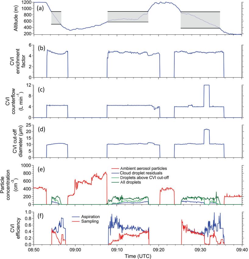
Figure 1. Comparison of spectral radiance in the nadir direction I ↑ measured by SMART, AISA Eagle/Hawk, and the Canon fisheye camera
on 27 May 2017 (flight no. 6). All data are convolved to the three spectral bands of the fisheye camera. Time series for all bands (a) and
scatter plots using the radiance of AISA Eagle/Hawk as reference (b) are shown. ∅ gives the mean and “Dev” the standard deviation of the
differences between the data sets. r denotes the Pearson’s correlation coefficient.
for AISA Eagle/Hawk, and 0.6 ms for the fisheye camera. diance. Therefore, the relative fractions of direct and diffuse
The regression of the radiances of the SMART Albedome- solar radiation were estimated using radiative transfer simu-
ter and AISA Eagle/Hawk (red dots in Fig. 1d–f) shows an lations (cloud free and cloud covered). The simulations were
offset in the range of 10 %, which is similar to previous mea- updated continuously based on available in-flight observa-
surement campaigns (Bierwirth et al., 2013; Ehrlich et al., tions and consider the temperature and humidity profiles and
2012). The red and green channel of the fisheye camera (blue the presence or absence of clouds. For the conditions dur-
dots in Fig. 1d–f) are comparable to the AISA Eagle/Hawk, ing ACLOUD, a 5 % uncertainty of the simulated fraction
while a significant difference of about 35 % on average is of direct radiation amounts to less than 1 % uncertainty of
observed for the blue channel. This comparison of the three the corrected downward irradiance. The upward solar radia-
instruments was used to inter-calibrate the fisheye camera in tion, as well as the upward and downward terrestrial radiation
order to provide a consistent data set. cannot be corrected for the aircraft attitude. However, these
components are characterized by a nearly isotropic radiation
3.3 Broadband solar and terrestrial radiation and field compared to the downward radiation and the effects of a
surface brightness temperatures misalignment are minimal for a nearly level sensor (Bucholtz
et al., 2008). To limit the remaining uncertainties due to the
Upward and downward broadband irradiances were mea- aircraft movement, measurements with roll and pitch angles
sured by pairs of CMP 22 pyranometers and CGR4 pyr- exceeding ±4◦ were removed from the data set.
geometers, covering the solar (0.2–3.6 µm) and thermal- To account for the slow response of the pyranometer and
infrared (4.5–42 µm) wavelength range, respectively. Both pyrgeometer, a correction of the instrument inertia time fol-
aircraft, Polar 5 and 6, were configured with an identical set lowing the approach by Ehrlich and Wendisch (2015) was ap-
of instruments and sampled with a frequency of 20 Hz. In sta- plied. Response times of 2 and 6 s (e folding time), character-
tionary operation, the uncertainty of the sensors is less than ized in laboratory measurements, were applied for the pyra-
3 %, as characterized by the calibration of the manufacturer nometer and pyrgeometer measurements. Assuming a typical
and evaluated by, e.g. Gröbner et al. (2014). For the airborne ground speed of 60 m s−1 and a flight altitude of 100 m, the
operation of the fixed mounted sensors, the misalignment of correction enables us to reconstruct horizontal fluctuations
the aircraft was corrected by applying the approach by Ban- up to scales of 3 m.
nehr and Schwiesow (1993) and Boers et al. (1998). This
correction is valid only for the downward direct solar irra-
www.earth-syst-sci-data.net/11/1853/2019/ Earth Syst. Sci. Data, 11, 1853–1881, 2019
1860                                                                                                 A. Ehrlich et al.: The ACLOUD data set

Figure 2. Time series of radar reflectivity profiles measured on 25 May 2017 (flight no. 23) for different processing steps: (a) raw data;
(b) after subtraction of mirror signal; (c) after speckle filter; (d) filtered data on a time–height grid; (e) corrected for sensor altitude, mounting
position, and pitch and roll angle; (f) remapping onto a constant vertical grid. The grey shading indicates the range of surface contamination
(≤ 150 m).

   During flights inside clouds, icing by super-cooled liquid                (MiRAC-P) with six channels along the strong water vapour
water droplets might have affected the radiation measure-                    absorption line at 183.31 GHz and two window channels at
ments after ascents and descents through the clouds. Using                   243 and 340 GHz. MiRAC-A is operated in a belly pod fixed
on-board video camera observations, the data were screened                   below the aircraft fuselage pointing about 25◦ backwards
for icing events when the solar downward irradiance ap-                      off nadir, while MiRAC-P is integrated in the cabin-pointing
peared artificially reduced. As this detection of icing was not              nadir. The cloud radar of MiRAC-A provides vertically
always reliable, uncertainties remain.                                       resolved profiles of the equivalent radar reflectivity. The
   Surface brightness temperature was measured by a nadir-                   vertical resolution depends on the chirp sequences and the
looking Kelvin infrared radiation Thermometer (KT-19).                       temporal resolution, which varied between 1 and 2 s. During
These measurements were converted into surface tempera-                      ACLOUD, three different settings with resolutions between
ture values assuming an emissivity of 1. This is justified                   4 and 30 m were used. A multi-step processing of the radar
due to the small impact of atmospheric absorption in the                     data was performed to correct disturbances in radar signal
wavelength range of 9.6 to 11.5 µm for which the KT-19 is                    due to the strong surface return and to convert them into
sensitive (Hori et al., 2006). With a sampling frequency of                  geo-referenced data taking the sensor’s mounting and the
20 Hz, the KT-19 resolves small scales of the surface tem-                   aircraft attitude into account (Mech et al., 2019). Figure 2
perature heterogeneities, such as observed in the case of                    illustrates the effect of the processing steps, which finally
leads in sea ice (Haggerty et al., 2003). The processed data                 lead to regularly gridded data, which become reliable 150 m
of the KT-19, pyranometer, and pyrgeometer were merged                       above ground level. The passive channels receive microwave
and published in a combined data set (Stapf et al., 2019,                    emission from the surface and the atmosphere. The 89 GHz
https://doi.org/10.1594/PANGAEA.900442).                                     channel is especially sensitive to the surface emission and
                                                                             the emission by liquid clouds. Over the open ocean, where
3.4    Active and passive microwave remote sensing                           the emissivity of the surface is low, this channel can be
                                                                             used to retrieve the liquid water path. The channels around
The Microwave Radar/radiometer for Arctic Clouds                             the 183.31 GHz water vapour absorption line can be used
(MiRAC; Mech et al., 2019) has been designed for op-                         to sense atmospheric moisture. The more the channels
eration on-board Polar 5. It consists of a single vertically                 are displaced from the absorption line centre, the lower
polarized Frequency Modulated Continuous Wave (FMCW)                         in the atmosphere the emitted radiation originates. The
cloud radar RPG-FMCW-94-SP, including a passive chan-                        combination of all spectral channels, therefore, provides
nel at 89 GHz (MiRAC-A) and a microwave radiometer

Earth Syst. Sci. Data, 11, 1853–1881, 2019                                                      www.earth-syst-sci-data.net/11/1853/2019/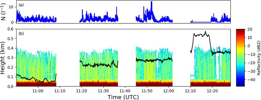
A. Ehrlich et al.: The ACLOUD data set                                                                                     1861

information about humidity from different layers. With            clouds (below 30 m above the ground) are excluded. Pro-
increasing frequency, larger snow particles can lead to a         files of attenuated backscatter coefficients and depolarization
brightness temperature depression due to scattering effects.      ratios are available on request and not yet included in the
The processed data of MiRAC-A and MiRAC-P were                    data set because the processing of the backscatter profiles
merged and published in a combined data set (Kliesch and          needs special treatment depending on their specific applica-
Mech, 2019, https://doi.org/10.1594/PANGAEA.899565).              tion (clouds or aerosol).

3.5   Remote sensing by lidar                                     3.6   Sun photometer

The active microwave profiling by MiRAC was comple-               The airborne Sun photometer with an active tracking sys-
mented by the Airborne Mobile Aerosol Lidar (AMALi) sys-          tem (SPTA) was installed under a quartz dome of Polar 5
tem (Stachlewska et al., 2010). This backscatter lidar has        to derive the spectral aerosol optical depth (AOD). It oper-
three channels: one unpolarized channel in the ultraviolet        ates a filter wheel with 10 selected wavelengths in the spec-
(UV) at 355 nm and two channels in the visible spectral           tral range from 367 to 1024 nm. To measure the direct so-
range at 532 nm (perpendicular and a parallel polarized). The     lar irradiance, the optics of the SPTA use an aperture with
backscattered intensities can be converted into attenuated        a field of view of 1◦ . With knowledge of the extraterrestrial
backscatter coefficients, depolarization ratio at 532 nm, and     signal the spectral optical depth of the atmosphere as well
the colour ratio (532–355 nm) to analyse cloud and aerosol        as spectral optical depth of aerosol was derived. The algo-
particles.                                                        rithm applied for the SPTA is based on Herber et al. (2002).
   During ACLOUD, AMALi was installed pointing down-              The extraterrestrial signal was calculated based on a Lan-
wards (except on flight no. 10 where it pointed in the zenith     gley calibration, which are performed regularly in a high
direction) through a floor opening of Polar 5, thus probing the   mountain area (Izana, Tenerife). The published data (Her-
atmosphere between the flight level and the surface. For eye      ber, 2019, https://doi.org/10.1594/PANGAEA.907097) were
safety reasons, AMALi was operated at flight levels above         screened for contamination by clouds to minimize an arti-
2700 m only. Overlap between the transmitted laser beam           ficial enhancement of the AOD by thin clouds. The cloud
and the receiving telescope is achieved for ranges larger than    screening algorithm applied a threshold of measured irradi-
235 m (Stachlewska et al., 2010). Data are recorded with          ance and made use of the higher temporal and spatial vari-
7.5 m vertical and 1 s temporal resolution. For consistency       ability of clouds compared to the rather smooth changes of
with the radar profiles, the AMALi data were converted into       aerosols properties (Stone et al., 2010).
“altitude above sea level” by using the GPS altitude. To im-
prove the signal-to-noise ratio, the profiles were averaged       3.7   Thermodynamic sounding
for 5 s temporal resolution, which yields a horizontal res-
olution of 375 m for typical aircraft speeds over ground of       The Advanced Vertical Atmospheric Profiling System
270 km h−1 .                                                      (AVAPS) was operated on Polar 5 to release dropsondes of
   The data processing eliminated the background signal,          type RS904 (Ikonen et al., 2010). The sondes measure ver-
which mainly results from scattered sunlight and electronic       tical profiles of air temperature, humidity, pressure, and the
noise. Additionally, a drift of the so-called base line of each   horizontal wind vector between the typical flight altitude of
channel was corrected for. Neglecting aerosol extinction, the     3–4 km and the surface. The vertical resolution of the pro-
attenuated backscatter coefficients for each channel were cal-    files is about 5 m, determined by the fall velocity of about
culated from the background-corrected signals by normaliz-        10 m s−1 and the sampling frequency of 2 Hz. The Atmo-
ing the measurements to a typical air density profile (Stach-     spheric Sounding Processing Environment (ASPEN, Version
lewska et al., 2005). For the ACLOUD campaign, data from          3.3-543) software package was used to correct the raw data
the AWIPEV station in Ny-Ålesund were used (Maturilli,            for the slow time response of the temperature sensor and
2017a, b).                                                        to remove the known humidity bias (Voemel et al., 2016).
   The published data set provides cloud top height derived       Data close to the aircraft, where the sensors did not yet ad-
from the preliminary lidar profiles. Clouds below the air-        just to the outside temperature, and invalid measurements
craft were identified from the attenuated backscatter coeffi-     were removed by the quality check of ASPEN (configura-
cients in the 532 nm parallel channel. Each height bin of the     tion set “research dropsonde”). To resolve fast temperature
profile, which exceeds the backscatter coefficients of a ref-     and humidity changes at the cloud top, the time response of
erence cloud-free section by a factor of 5, was labelled as       the sensors has been corrected by an alternative method fol-
cloud. Cloud top height was then defined as the highest alti-     lowing Miloshevich et al. (2004). A time response (e fold-
tude, which meets the above criterion for consecutive altitude    ing) of 4 s was applied to the temperature sensor and 5 s to
bins. In the published data set (Neuber et al., 2019, https:      the humidity sensor. Both data, processed by ASPEN and
//doi.org/10.1594/PANGAEA.899962), cloud tops close to            additionally corrected for the time response using the ap-
the aircraft (less than 100 m below the flight level) and low     proach by Miloshevich et al. (2004), are included in the pub-

www.earth-syst-sci-data.net/11/1853/2019/                                        Earth Syst. Sci. Data, 11, 1853–1881, 2019
1862                                                                                   A. Ehrlich et al.: The ACLOUD data set

lished data set (Ehrlich et al., 2019a, https://doi.org/10.1594/   the CDP-2 raw PNSD was computed by the probe manu-
PANGAEA.900204).                                                   facturer software, which applies the first solution of the Mie
                                                                   theory particle size determination. In the second step, raw
4     Instrumentation of Polar 6                                   PNSD has then been corrected using a Monte Carlo inver-
                                                                   sion method to ensure equiprobable values to all possible so-
Polar 6 was primarily equipped with in situ instruments char-      lutions of the Mie theory particle size determination. In or-
acterizing aerosol particles, cloud droplets, ice crystals, and    der to do so, the particle counts (Nraw ) from one raw size
trace gases (Table 2). Cloud particles were sampled with five      bin were uniformly distributed into a finer binning (Nfine ) for
different optical array and scattering probes. Using a counter-    a more precise particle size determination and a scattering
flow virtual impactor (CVI), the aerosol particles and cloud       cross section was computed for each Nfine . A diameter was
particle residuals were collected and characterized by the in      then randomly attributed to each count of Nfine using the dif-
situ aerosol instrumentation. The trace gas instrumentation        ferent solution given by the Mie theory with equiprobability,
measured concentrations of CO, CO2 , O3 , and water vapour.        and these diameters were distributed into the same original
Meteorological properties, including turbulent and radiative       size bins (Ncor ).
fluxes, were measured with an instrumentation identical to            The final calibrated PNSD are obtained by applying the
that operated on Polar 5 (see Sect. 3.1).                          calibrated sampling area and removing shattered particles,
                                                                   which are identified from the inter-arrival times. Prior to its
                                                                   use, the probe has been calibrated using glass beads for sizing
4.1     Cloud particle in situ measurements
                                                                   and a single-droplet generator (Lance et al., 2010; Wendisch
Four wing pylons are available on Polar 6, two on each             et al., 1996) for the sample area (0.32 mm2 ). Microphysical
wing. For ACLOUD five different probes were installed to           quantities such as LWC and effective droplet diameter Deff
sample cloud particle microphysical and optical properties:        were derived from the PNSD.
the Cloud Droplet Probe (CDP-2), the Cloud Imaging Probe
(CIP), the Precipitation Imaging Probe (PIP), the Small Ice        4.1.2   The Cloud Imaging Probe and the Precipitation
Detector Mark 3 (SID-3), and the Particle Habit Imaging and                Imaging Probe
Polar Scattering probe (PHIPS). Two configurations were ap-
plied. The combination of PIP, CIP, SID-3, and PHIPS was           The Cloud Imaging Probe (CIP) and Precipitation Imaging
operated during the first half of ACLOUD (flight nos. 8–           Probe (PIP) measure the size and the shape of cloud parti-
15). In the second half (flight nos. 16–24), the PIP was re-       cles (Baumgardner et al., 2011). Their measurement princi-
placed by the CDP-2 to improve the sampling of small cloud         ple is based on that of Optical Array Probes (OAPs, Knol-
droplets, which dominated the rather warm clouds observed          lenberg, 1976), which use the linear array technique to ac-
during ACLOUD. Bulk liquid and total water content (LWC,           quire two-dimensional black and white images of particles.
TWC) was measured on Polar 6 with a Nevzorov heated wire           As the particles pass through the laser they cast a shadow,
probe.                                                             which is recorded on a photodiode array and analysed for
                                                                   particle dimension and shape. According to the resolution
                                                                   of the photodiode and their quantity, the CIP and PIP have
4.1.1    The Cloud Droplet Probe
                                                                   nominal size ranges of 25–1550 µm (25 µm resolution and 64
The Cloud Droplet Probe (CDP-2) is a forward-scattering op-        diodes) and 100–6200 µm (100 µm resolution and 64 diodes),
tical spectrometer (size range 2–50 µm) using a single-mode        respectively. The particle size distribution of hydrometeors
diode laser at a wavelength of 0.658 µm (Lance et al., 2010;       are computed from the OAP images. The assessment of the
Wendisch et al., 1996). It is operated with anti-shatter tips to   median mass diameter (MMD) and the ice water content
reduce possible shattering artefacts (Korolev et al., 2011) and    (IWC) relies on the definition of the crystal diameter and
allows for the retrieval of particle by particle information.      its mass–diameter relationship. Two mass–diameter relation-
The instrument counts and sizes individual droplets by de-         ships were considered in the data set: Baker and Lawson
tecting pulses of light scattered from a laser beam in the near-   (2006), denoted with BL06, and Brown and Francis (1995),
forward direction (4–12◦ ). Sizes are accumulated in 30 bins       labelled with BF95. Following the approach by Crosier et al.
with variable widths. For ACLOUD, a 1 µm bin width was             (2011), non-spherical ice crystals were separated from liq-
chosen for small droplet sizes (2–14 µm), while larger cloud       uid droplets based on their circularity parameter (circular-
droplets (16–50 µm) were collected in 2 µm bins. The particle      ity larger than 1.25 and image area larger than 16 pixels).
diameter was deduced from the measurement using a scatter-         Only these non-spherical particle images were used for the
ing cross section to diameter relationship based on the Mie        computation of the “ice” phase. Possible contamination of
theory. This relationship is a non-monotonic function, which       shattering and splashing of ice and liquid particles on the
can give multiple solutions for one scattering cross section       instruments’ tips have been identified and removed using
measurement. Therefore, the particle number size distribu-         inter-arrival time statistics and image processing (Field et
tion (PNSD) was obtained in two consecutive steps. First,          al., 2006). Due to the large OAP measurement uncertainties

Earth Syst. Sci. Data, 11, 1853–1881, 2019                                         www.earth-syst-sci-data.net/11/1853/2019/
A. Ehrlich et al.: The ACLOUD data set 1863
for the smallest sizes, the first two PNSD size bins were re- methods described in Schnaiter et al. (2016). The particle
moved. A complete description of the data processing, in- shape is given in the form of nine Fourier coefficients yk (k =
cluding a discussion of the applied mass–diameter relation- 1. . .9) derived from the 2-D scattering pattern. Using these
ships can be found in Leroy et al. (2016) and Mioche et al. coefficients, the particles can be classified as columnar (max-
(2017). ima for y2 or y4 ) or hexagonal (maxima for y3 , y6 , or y9 ). In
In the CDP-2, CIP, and PIP data set published in the PAN- all other cases the particles are classified as irregular. The
GAEA database (Dupuy et al., 2019, https://doi.org/10.1594/ particle sphericity is given as a binary information, where all
PANGAEA.899074), the PNSDs of all instruments are stored particles having sphericity of 1 are classified as spheres. The
separately. In order to retrieve the most statistically reliable particle mesoscopic complexity is expressed with a complex-
PNSD, all particle images were used (suffix “ALL”). Trun- ity parameter ke that is an optical parameter varying roughly
cated images were extrapolated in order to estimate the par- between 4 to 6. Discussion of the link between the complex-
ticle diameter following Korolev et al. (2000). However, the ity parameter and the actual particle complexity can be found
classification of non-spherical particles was based on com- in Schnaiter et al. (2016). The SID-3 data sets available in
plete images only (suffix “ALL-IN”). Depending on the ap- PANGAEA contain 1 Hz particle PNSD (Schnaiter and Järvi-
plication, different definitions of the particle diameters can nen, 2019a, https://doi.org/10.1594/PANGAEA.900261) and
be applied when calculating the PNSD. This is why three the analysis results of the individual 2-D scattering pat-
PNSDs are provided, each based on one of three different di- terns (Schnaiter and Järvinen, 2019b, https://doi.org/10.
ameters (Dmax , Deq and Dcc ), which are defined as follows. 1594/PANGAEA.900380). For each detected particle, infor-
mation about the particle sphericity, shape, and mesoscopic
– Dmax or length is the maximum dimension originating crystal complexity are given.
from the image centre of gravity (see Leroy et al., 2016).
It was used in previous studies in the region (Jourdan
et al., 2010). 4.1.4 The Particle Habit Imaging and Polar Scattering
probe
– Deq or equivalent diameter is the diameter of the cir-
The Particle Habit Imaging and Polar Scattering (PHIPS)
cle, which has the same surface as the particle image.
probe is a combination of a polar nephelometer and a stereo-
Vaillant de Guélis et al. (2019) show that it is the least
scopic imager (Abdelmonem et al., 2016; Schnaiter et al.,
subjected to error in sizing due to out-of-focus defor-
2018) and analyses cloud particles in the size range 20–
mation of the image. Also, as it represents a surface, its
700 µm. The two parts of the instrument are combined by
property is closer to the scattering cross section and thus
a trigger detector so that both imaging and scattering mea-
more comparable to the CDP-2 measurements.
surements are performed on the same single particle. The
– Dcc or circumpolar diameter is the diameter of the circle polar nephelometer has 20 channels from 18 to 170◦ , with
encompassing the particle image. This is the diameter an angular resolution of 8◦ recording single-particle angu-
used in the BF95 mass–diameter relationship. lar scattering functions. The stereomicroscopic imager con-
sists of two camera and microscope assemblies with an an-
gular viewing distance of 120◦ acquiring a bright field stere-
4.1.3 The Small Ice Detector
omicroscopic image. The magnification of the microscopes
The Small Ice Detector Mark 3 (SID-3) records the spatial can be varied in the range from 1.4× to 9×, which corre-
distribution of the forward-scattered light from single cloud sponds to field of view dimensions ranging from 6.27 × 4.72
particles in the angular region of 5 to 26◦ as 2-D scattering to 0.98 × 0.73 mm2 , respectively. The optical resolution at
patterns (Hirst et al., 2001). Cloud particles passing a laser the highest magnification setting is about 2.3 µm. During
beam (wavelength 532 nm) are detected using two nested ACLOUD, two different magnifications of 6× and 8× were
trigger optics that have circular apertures with a half angle set for the two PHIPS microscopes of camera 1 and 2, re-
of 9.25◦ located at ±50◦ relative to the forward direction. spectively. The purpose of this setting is to capture a de-
The maximum camera acquisition rate is 30 Hz, whereas the tailed view of the particle in camera 2 while ensuring that
trigger detector has a maximum acquisition rate of 11 kHz. the same particle was completely captured by camera 1.
The trigger signal is recorded as a histogram that can be used Particles that were completely captured within the field of
to retrieve the cloud particle size distribution using size cal- view of either camera were analysed for their size, spheric-
ibration procedures described in Vochezer et al. (2016). The ity, and position within the image, as explained in Schön
PNSD covers a size range of 5–45 µm divided into 16 size et al. (2011). Furthermore, the images were manually as-
bins (2–5 µm resolution). From a subsample of the detected signed to different shape classes. The PHIPS data set avail-
particles, a high-resolution 2-D scattering pattern is acquired. able in PANGAEA contains separate image overviews for
These scattering patterns were analysed for the particle shape both cameras per flight (Schnaiter and Järvinen, 2019c, https:
and sphericity using methods described in Vochezer et al. //doi.org/10.1594/PANGAEA.902611). Further, it contains
(2016) or for the particle mesoscopic complexity using the single-particle angular light-scattering data for each recorded
www.earth-syst-sci-data.net/11/1853/2019/ Earth Syst. Sci. Data, 11, 1853–1881, 20191864 A. Ehrlich et al.: The ACLOUD data set
calculations require the true air speed, which was measured
by the five-hole probe installed at the nose boom of Polar 6.
Uncertainties of Nevzorov probes have been discussed by,
e.g. Wendisch and Brenguier (2013) and Schwarzenboeck
et al. (2009). The main uncertainty of the computed LWC
and TWC is associated with the estimates of the dry-air out-
put signal, which was determined manually right before and
after the in-cloud segments of the flights. During the in-cloud
segments, the dry-air signal is unknown and is obtained by
linear interpolation of the before- and after-cloud values. The
version of the Nevzorov probe installed on Polar 6 during
ACLOUD requires manual balancing of the probe, which is
done by an human operator during the flight. Some parts of
the data could not be recovered when the balancing was not
done on time by the operator. For the majority of clouds,
the liquid water content values obtained from the LWC sen-
Figure 3. Comparison of averaged PNSD derived from CPD-2, sor of the Nevzorov probe are in close agreement with es-
SID-3 and CIP during flight no. 20 on 18 June 2017. For CDP-2 timates obtained by integrating the droplet size distribution
the corrected and uncorrected PNSD produced by the manufacturer
measured by the CDP-2. The ice water content calculated
software are shown. For CIP, all three options to calculate the parti-
from the difference of TWC and LWC is highly uncertain in
cle diameter are presented.
mixed-phase clouds due to the small amount of cloud ice in
the majority of clouds observed during the ACLOUD cam-
particle. For a sub-sample of particles, the microphysical in- paign and, therefore, not included in the database (Chechin,
formation derived from the image analysis was combined in 2019, https://doi.org/10.1594/PANGAEA.906658).
a single ASCII file per flight.
4.2 Aerosol particle measurements
4.1.5 Combined cloud particle number size distributions
Ambient aerosol particles and cloud particle residuals were
When flown together (flight nos. 16–26), CDP-2, SID-3, and collected by two inlets on-board Polar 6. Their microphysi-
CIP data can be combined for merged PNSDs that cover a cal and chemical properties were measured inside the cabin
size range between 2 and 1550 µm. Figure 3 shows PNSD of by a suite of aerosol sensors (Table 2). A third and fourth in-
all instruments averaged over the entire flight of 18 June 2017 let provided ambient air for the in-cabin instrumentation of
(flight no. 20). Only data with liquid water content above trace gas analysis. The characteristics and the handling of the
1 mg m−3 were included. For the CDP-2, the uncorrected different inlets is discussed below in Sect. 4.4.
PNSD produced by the manufacturer software was also in-
cluded, which shows a significant overestimation of small 4.2.1 Aerosol particle number concentration and
droplets below 8 µm compared to the corrected version. The number size distribution
PNSD derived from SID-3 measurements agrees well with
the CDP-2 and both match the smallest bins of the CIP. For All aerosol particle sizes measured during ACLOUD refer
CIP, all three options to calculate the particle diameter are to dry aerosol because most particulate water evaporates in
presented. The choice of diameter definition mostly affects the sampling lines connecting the inlets and the instruments
ice crystals larger than 200 µm where the equivalent diame- due to the higher temperature inside the aircraft cabin. Two
ter Deq gives the lowest ice crystal concentrations (assuming ultra-high sensitivity aerosol spectrometers (UHSAS, Cai
smaller crystals), and the circumpolar diameter Dcc gives the et al., 2008) were operated either at different inlets (for si-
highest ice crystal concentrations (assuming larger crystals). multaneous measurements) or at the same inlet (for inter-
comparison). The flow rate was set to 50 mL min−1 . The UH-
SAS measures the number size distribution of particles with
4.1.6 Bulk liquid water content
diameters between 60 and 1000 nm by detecting scattered
A standard Nevzorov heated wire probe (Korolev et al., laser light divided in 100 user-specified size bins of variable
1998) was installed on the nose of Polar 6 to measure bulk size (2–30 nm resolution). From these measurements, the
liquid and total water content (LWC, TWC). The raw data mean particle diameter and the particle number concentra-
were averaged over 1 s intervals and processed to compute tion of a defined size range were derived. From the data eval-
the liquid water content based on the method described by uation it was inferred that the UHSAS-1 and the UHSAS-
(Korolev et al., 1998). For both sensors (total and liquid wa- 2 could reliably detect particles larger than 60 and 80 nm,
ter), the collection efficiency is assumed to be equal to 1. The respectively. During ACLOUD, the UHSAS-1 broke during
Earth Syst. Sci. Data, 11, 1853–1881, 2019 www.earth-syst-sci-data.net/11/1853/2019/You can also read