Machine learning techniques for observational n-of-1 studies

Quantified Sleep
 Machine learning techniques for observational n-of-1 studies
 Gianluca Truda
arXiv:2105.06811v1 [q-bio.QM] 14 May 2021

 Vrije Universiteit Amsterdam

 May 17, 2021

 Abstract
 This paper applies statistical learning techniques to an observational Quantified-Self (QS)
 study to build a descriptive model of sleep quality. A total of 472 days of my sleep data was
 collected with an Oura ring. This was combined with a variety of lifestyle, environmental, and
 psychological data, harvested from multiple sensors and manual logs. Such n-of-1 QS projects
 pose a number of specific challenges: heterogeneous data sources with many missing values;
 few observations and many features; dynamic feedback loops; and human biases. This paper
 directly addresses these challenges with an end-to-end QS pipeline for observational studies that
 combines techniques from statistics and machine learning to produce robust descriptive models.
 Sleep quality is one of the most difficult modelling targets in QS research, due to high noise and
 a large number of weakly-contributing factors. Sleep quality was selected so that approaches
 from this paper would generalise to most other n-of-1 QS projects. Techniques are presented for
 combining and engineering features for the different classes of data types, sample frequencies,
 and schema. This includes manually-tracked event logs and automatically-sampled weather
 and geo-spatial data. Relevant statistical analyses for outliers, normality, (auto)correlation,
 stationarity, and missing data are detailed, along with a proposed method for hierarchical
 clustering to identify correlated groups of features. The missing data was overcome using
 a combination of knowledge-based and statistical techniques, including several multivariate
 imputation algorithms. “Markov unfolding” is presented for collapsing the time series into a
 collection of independent observations, whilst incorporating historical information. The final
 model was interpreted in two key ways: by inspecting the internal β-parameters, and using
 the SHAP framework, which can explain any “black box” model. These two interpretation
 techniques were combined to produce a list of the 16 most-predictive features, demonstrating
 that an observational study can greatly narrow down the number of features that need to be
 considered when designing interventional QS studies.

 Keywords: Quantified-self, machine learning, missing data, imputation, n-of-1, sleep, Oura ring,
 prediction, supervised learning, biohacking, observational, longitudinal, time series, interpretable,
 explainable.
 Source code: github.com/gianlucatruda/quantified-sleep

 1

Contents
1 Introduction 4
 1.1 Specific challenges . . . . . . . . . . . . . . . . . . . . . . . . . . . . . . . . . . . . 4
 1.1.1 Establishing causal relationships . . . . . . . . . . . . . . . . . . . . . . . . 4
 1.1.2 Many heterogeneous data sources . . . . . . . . . . . . . . . . . . . . . . . . 5
 1.1.3 Human in the dynamic feedback loops . . . . . . . . . . . . . . . . . . . . . 6
 1.1.4 Wide datasets . . . . . . . . . . . . . . . . . . . . . . . . . . . . . . . . . . . 6
 1.1.5 Missing values . . . . . . . . . . . . . . . . . . . . . . . . . . . . . . . . . . 7
 1.1.6 Complexities of sleep . . . . . . . . . . . . . . . . . . . . . . . . . . . . . . . 7
 1.2 Terminology and notation . . . . . . . . . . . . . . . . . . . . . . . . . . . . . . . . 8

2 Data sources 8
 2.1 Sleep data . . . . . . . . . . . . . . . . . . . . . . . . . . . . . . . . . . . . . . . . . 8
 2.2 Supporting data . . . . . . . . . . . . . . . . . . . . . . . . . . . . . . . . . . . . . 9

3 Data wrangling 11
 3.1 Data ingestion . . . . . . . . . . . . . . . . . . . . . . . . . . . . . . . . . . . . . . 11
 3.2 Midnight unwrapping . . . . . . . . . . . . . . . . . . . . . . . . . . . . . . . . . . 11
 3.3 Transformations . . . . . . . . . . . . . . . . . . . . . . . . . . . . . . . . . . . . . 12
 3.4 Aggregation techniques . . . . . . . . . . . . . . . . . . . . . . . . . . . . . . . . . 13
 3.4.1 Aggregating temporal data . . . . . . . . . . . . . . . . . . . . . . . . . . . 13
 3.4.2 Aggregating location data with geohashes . . . . . . . . . . . . . . . . . . . 13
 3.5 Dataset concatenation . . . . . . . . . . . . . . . . . . . . . . . . . . . . . . . . . . 14

4 Analysis of dataset properties 15
 4.1 Time period . . . . . . . . . . . . . . . . . . . . . . . . . . . . . . . . . . . . . . . . 15
 4.2 Outliers . . . . . . . . . . . . . . . . . . . . . . . . . . . . . . . . . . . . . . . . . . 15
 4.3 Normality . . . . . . . . . . . . . . . . . . . . . . . . . . . . . . . . . . . . . . . . . 16
 4.4 Correlation . . . . . . . . . . . . . . . . . . . . . . . . . . . . . . . . . . . . . . . . 16
 4.4.1 Pairwise correlation with target . . . . . . . . . . . . . . . . . . . . . . . . . 17
 4.4.2 Hierarchical correlational clustering . . . . . . . . . . . . . . . . . . . . . . 18
 4.4.3 Autocorrelation . . . . . . . . . . . . . . . . . . . . . . . . . . . . . . . . . . 20
 4.5 Stationarity . . . . . . . . . . . . . . . . . . . . . . . . . . . . . . . . . . . . . . . . 21

5 Overcoming missing data 22
 5.1 Theory of missing data . . . . . . . . . . . . . . . . . . . . . . . . . . . . . . . . . . 22
 5.2 Analysis of missing data . . . . . . . . . . . . . . . . . . . . . . . . . . . . . . . . . 22
 5.3 Approaches to handle missing data . . . . . . . . . . . . . . . . . . . . . . . . . . . 24
 5.4 Knowledge-based filling . . . . . . . . . . . . . . . . . . . . . . . . . . . . . . . . . 24
 5.5 Imputation strategies . . . . . . . . . . . . . . . . . . . . . . . . . . . . . . . . . . . 25
 5.5.1 Univariate imputation . . . . . . . . . . . . . . . . . . . . . . . . . . . . . . 25
 5.5.2 Multivariate imputation . . . . . . . . . . . . . . . . . . . . . . . . . . . . . 25
 5.5.3 Multiple imputation . . . . . . . . . . . . . . . . . . . . . . . . . . . . . . . 25
 5.6 Baseline dataset with missing values . . . . . . . . . . . . . . . . . . . . . . . . . . 26
 5.7 Quantifying imputation distance . . . . . . . . . . . . . . . . . . . . . . . . . . . . 26

6 Collapsing time with Markov unfolding 28
 6.1 Markov assumption . . . . . . . . . . . . . . . . . . . . . . . . . . . . . . . . . . . . 28
 6.2 Markov unfolding . . . . . . . . . . . . . . . . . . . . . . . . . . . . . . . . . . . . . 29

 2

Quantified Sleep : CONTENTS Gianluca Truda

7 Model interpretation 30
 7.1 Interpreting model parameters . . . . . . . . . . . . . . . . . . . . . . . . . . . . . 30
 7.1.1 Regularised linear models . . . . . . . . . . . . . . . . . . . . . . . . . . . . 30
 7.1.2 Recursive feature elimination (RFE) . . . . . . . . . . . . . . . . . . . . . . 30
 7.2 Model-agnostic interpretation . . . . . . . . . . . . . . . . . . . . . . . . . . . . . . 31
 7.2.1 Shapley values . . . . . . . . . . . . . . . . . . . . . . . . . . . . . . . . . . 31
 7.2.2 SHAP . . . . . . . . . . . . . . . . . . . . . . . . . . . . . . . . . . . . . . . 32

8 Experiments 32

9 Results and discussion 34
 9.1 Effectiveness of Markov unfolding . . . . . . . . . . . . . . . . . . . . . . . . . . . . 34
 9.2 Comparison of imputation techniques . . . . . . . . . . . . . . . . . . . . . . . . . 36
 9.3 Predictive performance . . . . . . . . . . . . . . . . . . . . . . . . . . . . . . . . . . 38
 9.4 Model interpretation . . . . . . . . . . . . . . . . . . . . . . . . . . . . . . . . . . . 39
 9.4.1 Interpreting cross-validated RFE . . . . . . . . . . . . . . . . . . . . . . . . 39
 9.4.2 Interpreting cross-validated Lasso . . . . . . . . . . . . . . . . . . . . . . . . 40
 9.4.3 Interpreting model with SHAP . . . . . . . . . . . . . . . . . . . . . . . . . 41
 9.4.4 Combined interpretation . . . . . . . . . . . . . . . . . . . . . . . . . . . . . 43
 9.5 Feature explanation . . . . . . . . . . . . . . . . . . . . . . . . . . . . . . . . . . . 45

10 Limitations and future work 46
 10.1 Ground truth . . . . . . . . . . . . . . . . . . . . . . . . . . . . . . . . . . . . . . . 46
 10.2 Generalisability . . . . . . . . . . . . . . . . . . . . . . . . . . . . . . . . . . . . . . 46
 10.3 Markov unfolding . . . . . . . . . . . . . . . . . . . . . . . . . . . . . . . . . . . . . 46
 10.4 Imputation . . . . . . . . . . . . . . . . . . . . . . . . . . . . . . . . . . . . . . . . 47
 10.5 Interpretation . . . . . . . . . . . . . . . . . . . . . . . . . . . . . . . . . . . . . . . 47
 10.6 Hierarchical clustering . . . . . . . . . . . . . . . . . . . . . . . . . . . . . . . . . . 47

11 Conclusions 48

12 Practicalities 49
 12.1 Code and data availability . . . . . . . . . . . . . . . . . . . . . . . . . . . . . . . . 49
 12.2 Replicating this work . . . . . . . . . . . . . . . . . . . . . . . . . . . . . . . . . . . 49

A Appendices 53

 Page 3

Quantified Sleep : 1 INTRODUCTION Gianluca Truda

1 Introduction

Connected wearable devices are making personal data collection ubiquitous. These advances have
made Quantified-Self (QS) projects an increasingly-interesting avenue of research into personalised
healthcare and life extension [1]. Whilst there has been considerable progress made on the challenges
of collecting, storing, and summarising such data, there remains a gap between basic insights (e.g.
sleep duration) and the deeper kinds of analysis that allow for effective interventions [2] — e.g.
taking precisely 0.35 mg of melatonin 1-2 hours before bedtime to increase deep sleep by 22%.
There are also major challenges like missing values, few observations, feedback loops, and biological
complexity [3].
This QS study utilised 15 months of my personal data to find useful relationships between sleep
quality and hundreds of lifestyle and environmental factors. Multiple heterogeneous data sources
from both active and passive tracking systems were combined and preprocessed into a day-level
timeseries (§2). The study combines various techniques for feature engineering (§3), dataset analysis
(§4), missing value imputation (§5), temporal representation (§6), and model interpretation (§7).
These methods were evaluated for various learning algorithms through a series of experiments (§8).
The context of sleep quality is a good case study in observational n-of-1 research, as its challenges
generalise to other areas of QS research. Fig. 1 gives a graphical overview of the components of
this study.

 Data Analysis
source
 1
 Dataset variants Beta-parameter
 interpretation
 Preprocessing Grid search
 Data Knowledge- Missing data Best model and
 and over datasets Final interpretation
source Unified view based filling imputation dataset combination
 Aggregation and models
 2
 . SHAP interpretation
 .
 .

 Data
source Markov
 n unfolding

Figure 1: An overview of the data pipeline for this study, from disparate data sources to a final
interpretation of the effects on sleep quality.

1.1 Specific challenges
N-of-1 studies pose a number of unique challenges, but so do QS projects and observational studies.
At the intersection of all of these (Fig. 2) is the set of attributes that make this study uniquely
challenging. We begin by exploring these challenges.

1.1.1 Establishing causal relationships

The gold standard for experiments involving human subjects is the double-blind, randomised,
controlled trial (RCT). Such a study is interventional, typically having a single variable that is
manipulated, such as whether a subject receives a specific drug therapy. All other variables are
controlled by strict laboratory conditions, selective recruiting of participants, and rigorous protocols.
All of these measures help minimise various statistical and human biases that might affect the
outcome. This allows researchers to establish causal links between variables.

 Page 4

Quantified Sleep : 1 INTRODUCTION Gianluca Truda

 Observational N-of-1

 This
 study

 Day-level
 Quantified Self

Figure 2: Illustrative diagram of how this study sits at the intersection of observational research,
n-of-1 experiments, and day-level Quantified-Self (QS) research.

In total contrast, we have the n-of-1 QS study. This involves a single individual who designs,
administers, and is the subject of the experiments [1]. This makes the study very difficult to blind.
Confounding factors, ordering effects, and human biases are thus exacerbated when studying single
individuals. Moreover, it is often unclear at the outset what variables are relevant to study in
this way. This paper addresses these challenges by using a wide-spanning observational study to
identify interesting factors that can then be examined further in controlled studies. Techniques for
effectively executing these initial observational studies are the focus of this paper.
Whilst there are many challenges in observational n-of-1 research, it is also important to acknowledge
the many advantages. Firstly, n-of-1 studies offer something that RCTs cannot. Namely, direct
applicability to the subject in question. The cohort of an RCT is very carefully selected. The results
of these studies may, therefore, not fully generalise to the genetic, environmental, and psychological
attributes of other groups. For complex systems, n-of-1 studies allow data to be collected about the
specific individual in question [4]. Secondly, by beginning with a wide-ranging observational study,
n-of-1 research allows the subject to fit the study around their daily life. This further increases the
relevance of results, because they fit within the specific context that we are seeking to optimise.
The observational approach can also capture unexpected interactions between variables, which
helps identify the most relevant factors for future controlled studies.

1.1.2 Many heterogeneous data sources

The QS domain often requires combining multiple bespoke systems to collect both active and passive
data [2]. For instance, I log my caffeine intake actively using the Nomie app on my phone, but my
screen time is monitored passively by the RescueTime desktop software. For simple analytics, it is
sufficient to work with these sources in isolation. For more valuable multivariate analysis, however,
it is essential to unify the data sources and produce a combined dataset. This is challenging for two
reasons. Firstly, each source has its own schema for storing, processing, and exporting data. These
schema are usually specific to each system. Many tools often limit the level at which data can be
exported or analysed. Secondly, the nature and structure of the data differs from source to source.
For example, I keep track of caffeine intake by actively logging the date-time-stamp whenever I
drink coffee. This follows an event-based scheme, where each date-time-stamp is a record in a
relational database. Conversely, my sleep quality is passively measured and logged by my Oura
ring and stored (primarily) as a daily summary. To analyse the interactions between my caffeine

 Page 5

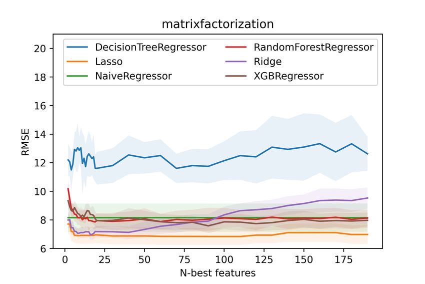
Quantified Sleep : 1 INTRODUCTION Gianluca Truda

intake and my sleep, I would need to reconcile these two schema by aggregating the caffeine logs to
daily summaries and then aligning the dates with the sleep summaries. Instead of events, I now
have daily features like average number of coffees, time of last coffee, etc. As more sources are
included in the dataset, the complexity of the processing and alignment increases.
This study addresses these challenge by parsing each data source into a dataframe [5], then aligning
these into a unified view. In order to do so, a number of feature aggregation and engineering
techniques were developed for this context (§3).

1.1.3 Human in the dynamic feedback loops

The very aspect of n-of-1 QS that makes it interesting also imbues it with challenges. Having a
human “in the loop” of the experiment introduces a number of biases and errors [6] that affect the
results [1]. It is typically too impractical to use any blinding methods in QS because we mostly
study multiple variables at once and cannot control for all the other factors. Self-blinding is quite
challenging even for a single independent variable [7]. For problems like sleep modelling, blinding
the subject is outright impossible, as almost all of the interesting variables include at least some
degree of subjectivity. For instance, it may be that tracking my sleep quality makes me more
anxious about my sleep, which in turn keeps me up longer and degrades my sleep efficiency. Or,
I may be less effective at estimating my mood and energy levels when I am sleep deprived. Or,
the act of logging caffeinated drinks or melatonin tablets may have a stronger placebo effect than
the actual substance. This means that even an accurate and explainable model will only be able
to describe the system it was based on — biases, feedback loops, and placebos included. It also
means that we need to take great care when interpreting our engineered features and the results we
produce.
Moreover, modelling dynamic systems with feedback loops requires time series techniques. Unfor-
tunately, these place constraints on the choice of models and the interpretations we can perform.
In this study, a technique called “Markov unfolding” (§6) is used to collapse the time series into
independent observations, allowing for historical data to be captured by non-temporal models.

1.1.4 Wide datasets

A fundamental challenge for n-of-1 QS projects is having insufficient data. Whilst many sensors
collect large quantities of data at high sample rates [1, 3], much of this is aggregated down to
summaries. This is because we are often interested in longer time periods, like hours or days [2]. In
this study, for instance, the focus is sleep quality. Because this is quantified daily, all data sources
must be aggregated to match this day-long window size of observations. A 200 Hz accelerometer
ultimately becomes dozens of engineered features summarising daily motion and activity. This has
the effect of collapsing low-dimensional, high-frequency data into high-dimensional, low-frequency
data. In other words, our dataset becomes wider than it is long. Naïve modelling of such a dataset
results in overparameterised models that are high in variance [8] and do not generalise [9, 10].
This challenge is addressed through the use of multiple feature selection techniques (§7.1.2), which
reduce dimensionality [3]. This is complemented by analysing the distributions of cross-validated
results to detect the ones that are robust across subsets of the data (§8).

 Page 6

Quantified Sleep : 1 INTRODUCTION Gianluca Truda

1.1.5 Missing values

Missing data is a major problem for modelling, because most techniques assume complete data [11].
The missing values either have to be filled in (imputed or interpolated) or discarded (dropped)
along with all other data for the observation. Imputation maintains the size and shape of the
dataset, but reduces the quality by introducing noise. Dropping introduces no additional noise, but
reduces the number of observations — making the dataset relatively shorter and wider — which
increases model variance.
N-of-1 QS studies exacerbate the problem of missing data dramatically. Because the study is
about a single individual, there are already fewer observations at the outset. Moreover, there is a
great deal of noise and complexity in the observations, as they are specific to the individual being
studied [7]. Additionally, QS projects involve data from multiple heterogeneous sources, and so
often require some experimentation with different pieces of software and hardware [2]. This results
in a dataset that has a great deal of missing values in one of a few characteristic types (§5.1).
Additionally, sensors and systems can fail, resulting in missing values scattered throughout the
data. Active-tracking sources are prone to poor adherence.
Fortunately, the unique nature of n-of-1 QS studies also allows us to utilise a collection of tricks
and tools that can overcome some of these missing data issues. This paper organises missing values
into distinct types (§5.1), inferring some from domain knowledge (§5.4), whilst others are imputed
using various sophisticated techniques (§5.5).

1.1.6 Complexities of sleep

This study’s target variable (sleep quality) posed some additional challenges. Not only is sleep a
complex and little-understood process [12], but it is one for which the subject is necessarily not
fully conscious, making measurement far more difficult. Many lifestyle factors have been shown
to affect sleep quality and quantity [13, 14, 15]. Poor sleep also impairs a subject’s ability to
accurately assess their sleep quality and quantity [16, 12]. Consumer-grade hardware for sleep
tracking is increasingly available due to wearable technology, but must infer sleep stages from
other physiological markers like heart rate, movement, heart rate variability (HRV), and body
temperature [17]. Unlike exercise tracking, the ground truth for sleep tracking is uncertain. This
adds additional noise to the target variable.
Sleep exists within a complex feedback loop with hundreds of other factors (including itself) [15, 12],
so a simple univariate analysis is clearly insufficient. Instead, this study is framed as a modelling
problem in which we wish to construct an explanatory model of sleep. To build the best possible
model, we convert the task to an optimisation problem under the framework of supervised learning:
models with a low prediction error on unseen (out-of-sample) data are more likely to have captured
the relevant variable interactions [10]. However, our end goal is not to make a good predictive
model. That is just an intermediate step to finding a good descriptive model. By interpreting
the model (§7), it is possible to find which variables are most influential in determining sleep
quality, highlighting potential avenues for further studies. For instance, the model may reveal that
melatonin consumption and timing of intense exercise are, together, two of the biggest predictors
of sleep quality. This information could then be used to design interventional n-of-1 studies that
specifically determine the effect size or optimal “dose” of each variable in isolation.

 Page 7

Quantified Sleep : 2 DATA SOURCES Gianluca Truda

1.2 Terminology and notation
Because machine learning sits at the intersection of a number of fields — statistics, computer
science, and software engineering — terminology is varied and overlapping. The goal of this paper
is to model a dependent variable (sleep quality) in terms of the independent variables that influence
it, such as caffeine consumption, exercise, weather, and previous sleep quality.
In this paper, the term feature will be used to refer to a preprocessed independent variable, whilst
target (feature) will be used for the dependent variable (sleep quality). For instance, caffeine
consumption is an input variable but, after preprocessing and aggregating, the hour at which
caffeine was consumed is a feature 1 . Input variables are often non-numeric, but all features are
numeric. Individual points in time (days) will be called observations 2 . When we dig beneath this
modelling view, datasets are organised as dataframes — m × n matrices with labels for each column
and row. Row i corresponds to an observation on a particular day. Column j correspond to a
timeseries for some feature. So columns are how we practically store our features whilst rows are
how we practically store our observations. This means that value xi,j is the single value in row i
and column j of our data matrix X ∈ Rm×n . So on day i, the jth feature had a value of xi,j .

2 Data sources

An overview of the data sources is found in Table 1. A detailed explanation follows.

2.1 Sleep data
The target variable for this study was sleep quality. This is a function of several sleep-related
variables that were captured using a second-generation Oura ring. The Oura ring is a wearable
device with sensors that measure movement, heartbeats, respiration, and temperature changes.
Being located on the finger instead of the wrist or chest, it can measure pulse and temperature
with greater sensitivity and accuracy, resulting in measurements suitable for sleep analysis [17].
Studies have found that the 250 Hz sensors of the Oura ring are extremely accurate for resting heart
rate and heart rate variability (HRV) measurement when compared to medical-grade ECG devices
[18]. This is likely due to the use of dual-source infrared sensors instead of the more common
single-source green light sensors when performing photoplethysmography [17]. Respiratory rate
was found to be accurate to within 1 breath per minute of electrocardiogram-derived measures by
an external study [19]. Internal studies [17] found the temperature sensor to be highly correlated
with leading consumer hardware, but uncorrelated to environmental temperature.
Combining the sensor data, the Oura ring has been found by a number of studies [20, 21, 22] to
produce reasonable estimates of sleep behaviour when compared to medical-grade polysomnography
equipment. This is remarkable given the significantly lower cost and invasiveness of the Oura ring.
Whilst all of the studies report that sleep detection has high sensitivity (and reasonable specificity),
the classification of different sleep stages diverges considerably from the polysomnography reference.
This, combined with the underlying opaqueness of sleep, made the target variable of this study noisy
 1 Because this paper may be of interest to readers from varying backgrounds, it should be noted that the term

feature is synonymous with terms like predictor, regressor, covariate, and risk factor ; whilst the target variable might
be known to others as a response variable, regressand, outcome, or label.
 2 In machine learning, observations are sometimes called examples or instances, but that is avoided in this paper

to prevent confusion.

 Page 8

Quantified Sleep : 2 DATA SOURCES Gianluca Truda

and uncertain. Despite this, the low costs and simplicity of the Oura ring make it an invaluable
tool for QS research in the domain of sleep.
The Oura API gives access to daily summaries generated from the raw sensor data. For this study,
the oura_score variable was of most interest, as it is intended to represent the overall sleep quality
during a sleep period. It is a weighted average of sleep duration (0.35), REM duration (0.1), deep
sleep duration (0.1), sleep efficiency (0.1), latency when falling asleep (0.1), alignment with ideal
sleep window (0.1), and 3 kinds of sleep disturbances: waking up (0.05), getting up (0.05), and
restless motion (0.05).

2.2 Supporting data
 • My electronic activities and screen time were tracked with the RescueTime application and
 exported as daily summaries of how much time was spent in each class of activity (e.g. 3h42m
 on software development).

 • My GPS coordinates, local weather conditions, and phonecall metadata were logged using
 the AWARE application for iOS and queried from the database using SQL. Local weather
 conditions and location information were logged automatically at 15-minute intervals (when
 possible). Phonecall metadata was logged whenever a call was attempted, received, or made.
 • Full timestamped logs of all caffeine and alcohol consumption were collected with the Nomie
 app for iOS. Logs were made within 5 minutes of beginning to consume the beverage. Caffeine
 was measured in approximate units of 100mg and alcohol was measured in approximations of
 standard international alcohol units.
 • Logs of activity levels and exercise measured on my phone were exported from Apple’s
 HealthKit using the QS Export app in the form of non-resting kilocalories burned at hourly
 intervals and activities (running, walking, etc.) logged as they began and ended.

 • Heart rate was recorded approximately once per minute3 on a Mi Band 4 and synchronised
 with AWARE via HealthKit.
 • My daily habits – meditation, practising guitar, reading, etc. – were captured (as Boolean
 values) daily before bedtime using the Way of Life iOS app.

 • My daily eating window (start and end times) was logged in the Zero app as daily summaries.
 • My mood and energy levels were logged at multiple (irregular) times a day in the Sitrus app.
 • A collection of spreadsheets were used to log the timestamps and quantities of sleep-affecting
 substances like melatonin and CBD oil.

 3 Higher frequencies were used during workout tracking and lower frequencies were used when the device was not

worn.

 Page 9

Kind Prefix Hardware Software Format Frequency Active/Passive Hoogendoorn-
 Quantified Sleep : 2

 Funk [3] categories
 Sleep oura Oura ring, 2nd gen. Oura API JSON Daily summaries Passive Physical
 Readiness oura Oura ring, 2nd gen. Oura API JSON Daily summaries Passive Physical
 Computer activity rescue Personal computer RescueTime CSV Daily summaries Passive Mental & Cognitive
 GPS coordinates aw_loc iPhone 8 AWARE v2 SQL ~15 mins Passive Environmental
 Barometric pressure aw_bar iPhone 8 AWARE v2 SQL ~15 mins Passive Environmental
 Local weather condi- aw_weather iPhone 8 AWARE v2 SQL ~15 mins Passive Environmental
 tions
 Phonecall metadata aw_call iPhone 8 AWARE v2 SQL ~15 mins Passive Social, Environmental
 DATA SOURCES

 Activity / Exercise hk iPhone 8, Mi Band 3, Apple HealthKit CSV Hourly summaries Passive Physical
 Oura ring
 Heart rate aw_hr Mi Band 3 AWARE v2 SQL ~1 min Passive Physical
 Caffeine and Alcohol nomie iPhone 8 Nomie app CSV Timestamped logs Active Diet
 Habits wol iPhone 8 Way of Life app CSV Daily Active Mental & Cognitive,
 Psychological, Situa-
 tional
 Eating / Fasting peri- zero iPhone 8 Zero app CSV Daily summaries Active Physical, Diet
 ods
 Mood and Energy mood iPhone 8 Sitrus app CSV Timestamped logs Active Psychological
 Melatonin use melatonin N/A Spreadsheet CSV Timestamped logs Active Diet
 CBD use cbd N/A Spreadsheet CSV Timestamped logs Active Diet
 Daily metrics daily ? N/A Spreadsheet CSV Daily logs Active Environmental, Situa-
 tional

 Table 1: The data sources used to build the dataset for this study. The prefix column indicates the string that the feature names in the
 dataset inherit from their source. These prefixes help associate features with their sources and allow easier grouping of features. ? Other
 prefixes: location, city, country, travelling.

Page 10
 Gianluca Truda

Quantified Sleep : 3 DATA WRANGLING Gianluca Truda

3 Data wrangling

The sampling intervals of the data sources ranged from below 1 minute to a full 24 hours. Much of
the data was necessarily at irregular intervals because it was an event log (e.g. having coffee or
taking melatonin). The data sources were all structured, but were a mix of temporal and numeric
types that required different feature engineering and aggregation techniques. Because the target
(sleep quality) was calculated at a daily interval, all the data needed to be up- or down-sampled
accordingly.
This section details how the heterogeneous data sources were ingested (§3.1), how custom feature
engineering was used to align (§3.2) and aggregate (§3.3) the different classes of time series, and
how the sources were concatenated into a unified dataset (§3.5).

3.1 Data ingestion
Each data source had its own bespoke data ingester that ultimately fed into a single unified view
from which features could be engineered to produce a dataset (Fig. 1). Each ingester is a function
responsible for reading a data source in its source format, transforming it into a dataframe, renaming
the columns with appropriate conventions and a descriptive prefix, then returning the dataframe.
This modularity allowed for iterative development during this study. It also allows the downstream
code to generalise to future studies on different data sources.

3.2 Midnight unwrapping
Because the data typically showed one sleep pattern per night, the window size for observations in
this study was necessarily one sleep-wake cycle (i.e. one day). Because sleep runs over midnight, it
was essential to select another time as the point around which each “day” was defined. To determine
this, temporal histograms of important activities like sleep, food consumption, and exercise were
plotted (e.g. Fig. 3). From this, a time of 05:00 was selected as the offset point. A window size of
24 hours was then applied from that reference. For instance, alcohol and caffeine consumed between
midnight and 05:00 count towards aggregates for the previous day. This simple technique preserves
causal relationships between input features and the target, as the order of events is preserved.

Figure 3: Temporal histograms for for alcohol and caffeine consumption, illustrating how a reference
time of 05:00 was selected for midnight unwrapping.

 Page 11

Quantified Sleep : 3 DATA WRANGLING Gianluca Truda

The summary date (based on 05:00 offset) was generated for each timestamp in each data source. For
instance, if alcohol was logged at 2020-04-07 01:03:41, the summary date was set to 2020-04-06.
All records were then grouped on that summary date attribute, with specific time-domain aggrega-
tions applied over the attributes to produce numerical features. This was informed by intuition
and domain knowledge and thus the aggregations varied across data sources.

3.3 Transformations
The unified dataset required all sources to be sparse daily summaries. This required aggregations
and interpolations. The data sources fell into three groups:

 1. Daily summaries: those sources that were already daily summaries (e.g. Oura, Zero,
 RescueTime). These required no further adjustment, provided their datestamp format was
 correct.
 2. Event logs: those that were records of the date and time that events occurred (e.g. caffeine,
 alcohol, melatonin, calls). There sources needed to be pivoted into wide format. The dates
 were then interpolated to daily summaries. Events occurring on the same day were aggregated.
 3. Intra-day samples: higher-frequency records (e.g. weather, location, heart rate). These
 sources needed aggregation to produce daily summaries.

Fig. 4 illustrates how such transformations would take place using highly-simplified scenarios.

 Date Deep sleep REM sleep Score

 2020-05-02 138 78 73

 Daily summaries 2020-05-03 102 113 81

 2020-05-04 192 109 86

 Date Time Event

 2020-05-02 08:12 Coffee
 Pivoting & Date Coffee Alcohol Date Deep sleep REM sleep Score Coffee Alcohol HR avg. HR std.
 aggregating
 2020-05-02 09:45 Coffee 2020-05-02 2 0 2020-05-02 138 78 73 2 0 74 32

 Event logs
 2020-05-03 22:17 Alcohol 2020-05-03 0 1 2020-05-03 102 113 81 0 1 78 29

 2020-05-04 09:01 Coffee 2020-05-04 1 0 2020-05-04 192 109 86 1 0 92 43

 Date Time Heart rate

 2020-05-02 00:01 63
 Date HR avg. HR std.
 Aggregating
 2020-05-02 00:02 65 2020-05-02 74 32

 Intra-day samples
 ...

 2020-05-03 78 29

 2020-05-04 23:58 92 2020-05-04 92 43

 2020-05-04 23:59 81

Figure 4: Toy examples of how the three kinds of data source in this study were transformed prior
to concatenation into the unified dataset.

 Page 12

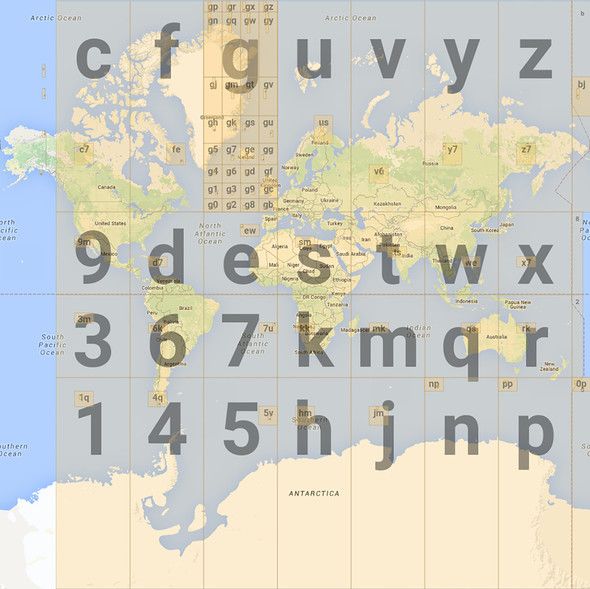
Quantified Sleep : 3 DATA WRANGLING Gianluca Truda

3.4 Aggregation techniques
When collapsing event logs and intra-day samples into daily summaries, aggregation functions
summarise the distribution. The choice of aggregation functions needs to consider the original data
source and the downstream learning pipeline.
For continuous variables (e.g. heart rate), standard summary statistics — minimum, mean,
maximum, standard deviation — capture the shape of the data well. This is particularly true when
the variable is close to a normal distribution, which many QS sources are. For categorical variables,
one-hot encoding and summation were used to aggregate data. For event logs (e.g. coffee and
alcohol consumption), counts are the most intuitive aggregation. Because the times that the events
took place is also important, specialised temporal aggregation techniques were needed.

3.4.1 Aggregating temporal data

For event logs, the hour of occurrence was encoded as a numeric feature along with the quantity,
allowing aggregation with min, max, and range functions. Hourly resolution is a reasonable level
given the inherent noise in the data.
Caffeine data is shown by way of an example:

 Summary date Value sum Hour min Hour max Hour range
 2020-06-12 2.0 12 14 2
 2020-06-13 1.0 13 13 0
 2020-06-15 2.0 11 13 2

Because midnight unwrapping had been applied, the net hour of occurrence was used. So having a
last beer at 1AM on Saturday would result in the net_hour_max feature on Friday having a value
of 25.

3.4.2 Aggregating location data with geohashes

High-frequency GPS data has huge potential for building information-rich features, but poses two
major challenges. Firstly, not all GPS measurements have the same level of accuracy, due to signal
availability and power-saving measures. Secondly, comparing or aggregating coordinates is difficult
and ill-defined. One solution is to manually define regions as places of interest and calculate which
GPS coordinate pairs fall within those regions. This proves to be very computationally expensive
and time consuming. Instead, this study used the geohash system [23] (Fig. 5).
Geohashing recursively divides the earth into 32-cell grids that are each codified with an alphanumeric
sequence. Because geohashes are based on the mathematics of z-order curves, they offer some useful
properties like arbitrary precision and fast encoding. For example, the GPS coordinates of the Vrije
Universiteit can be mapped to a level-6 geohash: (52.3361, 4.8633) → u173wx, which corresponds
to a rectangle with an area of 0.7 km. But by simply truncating the last 3 characters, we can “zoom
out” to u17, which covers the northern half of the Netherlands.

 Page 13

Quantified Sleep : 3 DATA WRANGLING Gianluca Truda

Figure 5: Illustration of the geohash system and example of the level-6 geohash for the Vrije
Universiteit [24].

The variable precision of geohashes helps overcome the GPS accuracy problem. Reducing pairs of
GPS co-ordinates to single alphanumeric strings with well-defined neighbourhood properties solves
the aggregation problems of GPS data.
The geohash encode function was mapped over all 61 000 GPS values in the dataset to generate the
level-12 geohashes in seconds. By simply truncating digits from the ends of these level-12 geohashes,
features were generated for levels 5 through 9. These levels correspond to blocks ranging from
25m2 to 25km2 , capturing location information at a variety of resolutions.
With this in place, daily aggregation was performed in two ways: (1) by counting the number of
unique geohashes from each level (5-9) for that day, (2) by finding the 10 most common level-5
geohashes over the entire dataset and counting the proportion of logs that matched each in that
day. This produced 15 features that summarised the locations and movements of the day in an
efficient format.

3.5 Dataset concatenation
All the preprocessed data sources were sequentially concatenated on the summary date column
using a left join operation. The sleep dataframe was used as the starting object. This served two
purposes. Firstly, it prevented the need for interpolating dates, as the sleep data was complete.
Secondly, it automatically resulted in all rows being trimmed to match the start and end of the
target feature (contained in the sleep data). This produced a unified dataset with 789 observations
(rows) and 309 columns, of which 271 were numeric features.
Because the data from the Oura ring contained numerous linear components of the target feature,
there was a risk of data leaks. For instance, oura_yesterday_total alone contributes 35% of
the oura_score target. But these variables were relevant to predicting future nights of sleep. To
remedy this, all variables with the oura_ prefix were copied, shifted one day later, and re-prefixed
with sleep_yesterday_. Before fitting the model, the features with the oura_ prefix were always
dropped. This way, each observation had no features leaking information about the target, yet still
included useful information about prior sleep behaviour.

 Page 14

Quantified Sleep : 4 ANALYSIS OF DATASET PROPERTIES Gianluca Truda

4 Analysis of dataset properties

4.1 Time period
The subset of the data used in this study ran for 472 days from mid-October 2019 to mid-January
2021. Some 65% of this time was under various restrictions due to the Covid-19 pandemic. This
meant much less variety in location and much more consistent patterns of behaviour, due to the
stay-at-home orders. This formed a natural experiment by keeping many factors consistent from
March 2020 to December 2020.
On one hand, this produced a more “controlled” experiment, with fewer free variables. On the
other hand, the unique circumstances mean that the results may not generalise as well. Moreover,
a lack of variability in features makes them less useful to a predictive model [10]. This can result in
highly-relevant variables being absent in the final model because they remained consistent during
the course of the lockdown. To mitigate this, data from 5 months of pre-pandemic conditions was
retained.

4.2 Outliers
It is essential to differentiate variational outliers from measurement-error outliers [3]. The former
are a legitimate result of natural variation in a system and must be retained in order to build a
fully-descriptive model. The latter are a result of failed sensor readings, corrupted data, or erroneous
data entry. These measurement errors add noise to the dataset that makes it more challenging to
fit a model to the underlying signal. They should therefore be removed. Unfortunately, it is often
difficult to differentiate the two types of outlier. To err on the side of caution, minimal outlier
removal was used in this study.
The focus of the study was sleep quality, so the most relevant sleep features were assessed to detect
outliers. By inspecting the distributions and linear relationships in the sleep data4 , the presence
of some outliers was apparent. Both the sleep efficiency and overall sleep score were negatively
skewed — with potential outliers in the left tail.
Chauvenet’s criterion is a technique to find observations that have a probability of occurring lower
than cN 1
 , where N is the number of observations and c is a strictness factor [3]. Chauvenet’s
criterion (c = 2) identified a total of 6 outliers across the 4 key sleep features: score, total, efficiency,
duration. All but one of these outliers pre-dated the intended timespan of the study, and that
outlier was removed.
For the non-target features, distribution plots and 5-number summaries were inspected to detect
erroneous measurements. For instance, a heart rate of 400 would have been clearly erroneous. No
values were deemed obvious errors5 .

 4 See
 Fig. 24 in the Appendices.
 5 It
 is, of course, possible that some data-entry errors or measurement errors made it past this conservative filter,
adding further noise to the data.

 Page 15

Quantified Sleep : 4 ANALYSIS OF DATASET PROPERTIES Gianluca Truda

4.3 Normality
Many learning algorithms assume that the target feature is normally distributed [25, 26]. If it
significantly differs from a normal distribution, we can either (1) normalise the target feature, or
(2) apply a transformation to the model predictions to map them onto the same distribution as
the target feature. Neither of these are ideal. Normalising the target feature makes our model
predictions harder to interpret [27]. Transforming the predictions can introduce a number of errors
and points of confusion.

Figure 6: Histogram showing the distribution of the target feature for the time period of the study:
oura_score. The median is indicated with a green vertical line. The mean is indicated with a
dashed red line. We can see that they are almost identical. Dotted black lines indicate one standard
deviation (σ) in either direction of the mean.

The target feature (oura_score) followed the general shape of a normal distribution, but with a
skewness of −0.325 and an excess kurtosis of 0.154, indicating thin tails and a negative skew (Fig.
6). We know that the target is bounded by [0, 100] and sleep behaviour generally regresses to the
mean [15], so there is little chance that the population distribution is extreme [28], even if it is
slightly skewed. These heuristics, along with the desire to keep the model interpretable, informed
the decision not to transform the target feature.

4.4 Correlation
It is important to understand how features linearly relate with one another (correlation) and with
themselves at different points in time (autocorrelation). If features that share a source are highly
correlated, we may want to combine them or discard one of them, as this maintains most of the
same information (and interpretability), whilst reducing the number of features our model needs to
process [25]. More importantly, features that are correlated with the target are strong candidate
features for our final model.

 Page 16

Quantified Sleep : 4 ANALYSIS OF DATASET PROPERTIES Gianluca Truda

4.4.1 Pairwise correlation with target

At first, we consider only correlations of each feature to the target (Fig. 7).

 Correlation of sleep variables with target (oura_score) Correlation of other variables with target (oura_score)
 oura_score city_Cape Town
 country_ZAF
 oura_ready_score_previous_nigh daily_week_no.
 oura_total daily_month
 aw_weather_temperature_min_std
 oura_score_total aw_weather_temperature_max_std
 oura_duration aw_weather_temperature_std
 wol_no_caffeine_after_3pm
 oura_score_rem wol_caffeinated_drinks_

Quantified Sleep : 4 ANALYSIS OF DATASET PROPERTIES Gianluca Truda

linear sum over several of these features. Curiously, a few sleep-related features had no direct
correlation with sleep score. Notably, those related to respiration rate and temperature.
The bedtime feature had a strong negative correlation with the target (r ≈ −0.6), which is likely
because it is considered as part of the ideal sleep window calculation that comprises 10% of the
sleep score. It was important to remove features like this from the dataset prior to training the
model, in order to prevent data leaks.
The non-sleep features had much weaker correlations with sleep score (−0.3 ≤ r ≤ 0.3), highlighting
that there were no obvious candidate features. The strongest correlations fell into the location,
weather, and caffeine categories. Notably, time-related features like the week number and month
number showed a notable correlation to sleep quality (r ≈ 0.2), indicating some trend or seasonality.
This would also explain why weather and location features showed strong correlations with the
target. Analysis of data stationarity is an essential step (§4.5).

4.4.2 Hierarchical correlational clustering

It is also important to consider how features might correlate with each other. For small numbers of
features, correlation matrices are ideal for such analysis. However, these graphics become difficult to
interpret when there are more than a dozen features. Instead, this study made use of agglomerative
clustering of features by their correlations to produce a dendrogram (Fig. 8).
The dendrogram was generated as follows: First, the features were filtered to only consider those
with less than 10% of their values missing. Each of the n features then had its absolute Pearson
correlation to each other feature calculated, producing an n × n correlation matrix. Next, the
pairwise Euclidean distances between each row of absolute correlations were calculated. Hierarchical
clustering was performed on these pairwise distances using the Nearest-Point algorithm. These
clusters were then plotted as a coloured dendrogram (Fig. 8).
This hierarchical approach to correlations between features is immensely useful and offers more
intuitive interpretations than a standard correlation matrix. By summarising the correlations
between all n × n pairs of features into distances in n-dimensional space, the complexity of the
relationships is interpreted for us. This highlights groups of features that are strongly correlated
with one another but not with other clusters of features. Moreover, we can use the dendrogram
representation to interpret just how correlated subsets of features are. This is immensely useful for
validating (and refining) feature engineering in order to achieve the higher sample efficiency needed
to model wide QS data.
In Fig. 8 we can see that the hourly movement data (prefix hk_act_) clustered together in chunks
of time and was highly correlated with aggregation features for this data. Specifically, we can
see that movement between the hours of 1 and 7 was very highly correlated and therefore also
highly correlated with their mean (hk_act_night_mean) (Fig. 8b). This tells us that most of the
(linear) information about nighttime movement can be captured from a single feature that averages
over the hourly features. We can also notice that there was low correlation between different time
windows of movement features. The morning, afternoon, and evening features clustered within
their time windows but not across them (Fig. 8c). This tells us that the different windows of time
throughout the day — morning, afternoon, evening, night — capture different information that
might be relevant to our model.
A final observation from the dendrogram is that location data formed a number of related, but
strongly-separated clusters. Geohashes gave similar information and were clustered (Fig. 8e), but
were very far from the cluster of features relating to city, country, and hemisphere (Fig. 8d). This
suggests that two levels of resolution are important — frequent changes in location at a resolution
of metres, and infrequent changes in location at a resolution of kilometres.

 Page 18

Quantified Sleep : 4 ANALYSIS OF DATASET PROPERTIES Gianluca Truda

 a.

 b.

 c.

 d.

 e.

Figure 8: Dendrogram of hierarchical correlational clustering for all features with low missing
data. Each of the n features were clustered based on their distance in n-dimensional space to other
features from the n × n correlation matrix. The dendrogram shows features on the vertical axis
and pairwise Euclidean distance on the horizontal axis. Vertices indicate where clusters join into
superclusters. The distance between clusters is represented by their vertical distance on the vertical
axis. Colour-coding is used to illustrate primary clusters based on a 70% similarity threshold. Note
that some feature names are replaced with location x to protect private data.

 Page 19

Quantified Sleep : 4 ANALYSIS OF DATASET PROPERTIES Gianluca Truda

4.4.3 Autocorrelation

Autocorrelation can be detected by computing the correlation between a feature and a copy of
the feature where values are shifted (lagged) by 1 or more points. Autocorrelation gives us an
indication of how well a feature predicts its own future values [29]. This was immensely useful in
this study because of the inherent time series nature of most QS data. Behavioural and biological
patterns often have periodic variations or trends over time. For example, it is common for people
to dramatically shift their sleeping patterns on weekends compared with weekdays. This can often
be detected by spikes in autocorrelation at intervals of 6-7 days — last week somewhat predicts
this week. For this study, the autocorrelation of each feature was analysed for varying shifts (lags)
up to 25 days. Four interesting patterns are presented in Fig. 9.

 (a) No autocorrelation. (b) Trending autocorrelation.

 (c) Periodic autocorrelation. (d) Trending autocorrelation.

Figure 9: Notable autocorrelation patterns observed across features. Each plot shows the correlation
on the vertical axis and the lag (in days) on the horizontal axis. The shaded regions represent
a 95% confidence interval for the null hypothesis at each lag level, so values that fall within this
region are unlikely to be significant.

We can see that the target feature (oura_score) had a very low degree of autocorrelation (Fig.
9a). This is extremely surprising, as it implies that previous sleep quality does not have a strong
linear relationship to current sleep quality. This highlights how difficult the task of predicting sleep
quality is. Interestingly, a lag of 1 day had a small negative correlation with the target (r1 ≈ −0.2).
This suggests that sleep oscillates in quality on adjacent nights. We can also see that some features
showed a clean trend of autocorrelation with respect to lag (Fig. 9b and 9d). This is to be expected

 Page 20

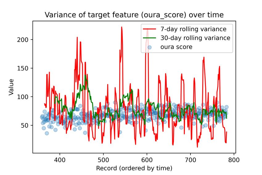
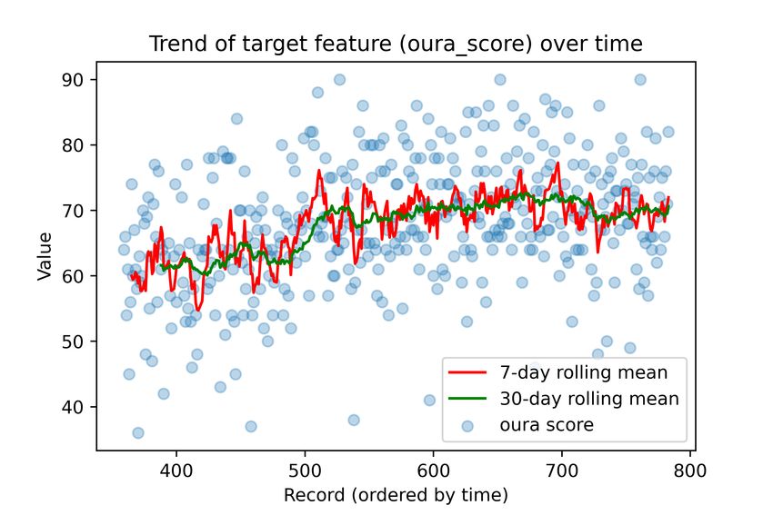
Quantified Sleep : 4 ANALYSIS OF DATASET PROPERTIES Gianluca Truda

of a number of features, such as habits and temporally-derived features like sleep_balance. What
is worth noting is the lag point at which the autocorrelation becomes statistically insignificant.
This gives us a rough indication of how many days of history may be relevant for our model.
Finally, we can see that some features displayed prominent periodicity (Fig. 9c). Productivity time
is derived from time spent on my laptop working with specific software or websites that are marked
as productive. We can see from the spikes in the plot that the periodicity had a peak-to-peak
length of exactly 7 days. This makes a great deal of sense, as my productivity levels are highly
influenced by the day of the week.

4.5 Stationarity
A key principle of modelling time series data is that it should be stationary. Specifically, it should
exhibit no periodicity or trends, leaving only irregular variations that we attempt to predict using
other features [3]. However, most real-world data is not stationary. As we have already seen, many
of the relevant features in this dataset are periodic.

 (a) Trend of mean for target. (b) Trend of variance for target.

Figure 10: Scatterplots of target features (oura_score) over time (indexed observations). The left
figure superimposes trends of the 7- and 30- day rolling mean. The right figure superimposes trends
of the 7- and 30- day rolling variance.

The augmented Dickey-Fuller test can be used to assess the stationarity of a sequence of data [30].
This test was applied to each feature in the dataset. A total of 34 input features were found to be
non-stationary (p > 0.05). Many of these were explicitly temporal features like the year, month, or
day. Many were naturally non-stationary data like weather patterns.
What we are most concerned with, however, is whether the target feature is stationary. If not,
techniques like statistical differencing need to be applied before building a model [3]. Unfortu-
nately, such applications make interpretation much more difficult. Fortunately, the target feature
(oura_score) was found to be stationary with reasonable confidence (p < 0.01). This means that
variations had no major periodic or trending patterns. This is illustrated visually with rolling
averages of both the mean and variance in Fig. 10. This was very fortunate for this study, as the
interpretation step is easier if we do not have to transform the target feature. This stationarity
of the sleep features was likely a happy result of the pandemic conditions. The data included for
modelling begins from October 2019. When including data back to December 2018, the target was
less likely to be stationary (p ≈ 0.09).

 Page 21

Quantified Sleep : 5 OVERCOMING MISSING DATA Gianluca Truda

5 Overcoming missing data

5.1 Theory of missing data
There are three main types of missing data identified in the statistics literature [31]. Understanding
their different properties is integral to selecting robust imputation techniques for filling in the
missing values [11].
Missing completely at random (MCAR): Missing values are considered MCAR if the events
that caused them are independent of the other features and occur entirely at random. This means
that the nullity (missingness) of the values is unrelated to any of our study features and we can
treat the data this is present as a representative sample of the data as a whole. Unfortunately,
most missing values are not MCAR [11].
Missing at random (MAR): Despite the name, MAR occurs when the nullity is not random,
but can be fully accounted for by other features that have no missing values. For instance, I did not
explicitly log the city where I slept every night, but the data is MAR because it is fully accounted
for by the date index and geohash features, from which I can accurately infer the missing values for
the city.
Missing not at random (MNAR): Data is MNAR when the nullity of the value is related to
the reason that it is missing. This makes the dataset as a whole biased. For instance, I am more
likely to forget to log my mood when I am very happy or utterly miserable. The missing extreme
values in the data are thus MNAR.

5.2 Analysis of missing data
The absence of data points is a major factor in Quantified-Self (QS) projects [3], especially when
combining data from multiple sources. An upfront analysis of the quantity and distribution of
missing values is essential before missing values can be rectified. Missing data matrices are an
invaluable visualisation in this regard. They give an impression of the dataset in the same rows-as-
observations and columns-as-features format that we are accustomed to, with shading to indicate
where data is present. In Fig. 11, the entire dataset is rendered as on of these matrices using the
superb missingno library [32]. It is important to note that this version of the dataset included more
than the 15-month timeline of the final dataset. This was for illustrative purposes. Much of the top
half of the dataset was ultimately discarded before modelling. In Fig. 12, the columns are grouped
by the source prefix (Table 1) in order to get a better understanding of which data sources are to
blame for which missing data. When combining columns from the same source, missing values took
precedence. In other words, the simplified matrix represents the worst-possible combination of the
columns from that source, in terms of nullity.
Anecdotally, these patterns are typical of multiple-source QS projects. New data sources are added
over time, whilst others fall out of use. Some data is tracked very consistently (often automatically),
whilst many of the manually-tracked sources have short sequences of missing values spread all over
— due to poor adherence to tracking protocols.
We can see from the missing data matrices that the sources used changed dramatically over time.
The AWARE (aw), Nomie, and Zero sources were only adopted later on. Fortunately for the focus
of this study, the sleep data (oura) was complete and had no missing data, as it was automatically
tracked and the ring was worn every night. By having a target feature free of missing data, this
study was well-positioned to mitigate the missing data in the other features.

 Page 22

Quantified Sleep : 5 OVERCOMING MISSING DATA Gianluca Truda

 1 123

 285

 789

Figure 11: Missing data matrix for the entire raw dataset. The vertical axis represents rows in the
dataset (corresponding to daily observations). The horizontal axis represents columns in the dataset
(corresponding to features). The dashed blue line indicates the start of the period of time considered
for this study. The sparkline on the right indicates the general shape of the data completeness,
with the rows of minimum and maximum nullity labelled with a count of the non-missing values in
the rows.

Figure 12: Missing data matrix for groups of features in the raw dataset. The vertical axis represents
rows in the dataset (corresponding to daily observations). The horizontal axis represents columns
in the dataset (corresponding to features). The dashed blue line indicates the start of the period
of time considered for this study. The sparkline on the right indicates the general shape of the
data completeness, with the rows of minimum and maximum nullity labelled with a count of the
non-missing values in the rows. The column names are the prefixes of each source (see Table 1).

 Page 23