Large-scale features of Last Interglacial climate: results from evaluating the lig127k simulations for the Coupled Model Intercomparison Project ...
←
→
Page content transcription
If your browser does not render page correctly, please read the page content below
Clim. Past, 17, 63–94, 2021
https://doi.org/10.5194/cp-17-63-2021
© Author(s) 2021. This work is distributed under
the Creative Commons Attribution 4.0 License.

Large-scale features of Last Interglacial climate: results from
evaluating the lig127k simulations for the Coupled Model
Intercomparison Project (CMIP6)–Paleoclimate Modeling
Intercomparison Project (PMIP4)
Bette L. Otto-Bliesner1 , Esther C. Brady1 , Anni Zhao2 , Chris M. Brierley2 , Yarrow Axford3 , Emilie Capron4 ,
Aline Govin5 , Jeremy S. Hoffman6,7 , Elizabeth Isaacs2 , Masa Kageyama5 , Paolo Scussolini8 , Polychronis C. Tzedakis2 ,
Charles J. R. Williams9 , Eric Wolff10 , Ayako Abe-Ouchi11 , Pascale Braconnot5 , Silvana Ramos Buarque12 , Jian Cao13 ,
Anne de Vernal14 , Maria Vittoria Guarino15 , Chuncheng Guo16 , Allegra N. LeGrande17 , Gerrit Lohmann18 ,
Katrin J. Meissner19 , Laurie Menviel19 , Polina A. Morozova20 , Kerim H. Nisancioglu21,22 , Ryouta O’ishi11 ,
David Salas y Mélia12 , Xiaoxu Shi18 , Marie Sicard5 , Louise Sime15 , Christian Stepanek18 , Robert Tomas1 ,
Evgeny Volodin23 , Nicholas K. H. Yeung19 , Qiong Zhang24 , Zhongshi Zhang16,25 , and Weipeng Zheng26
1 Climate   and Global Dynamics Laboratory, National Center for Atmospheric Research, Boulder, 80305, USA
2 Environmental   Change Research Centre, Department of Geography, University College London,
London, WC1E 6BT, UK
3 Department of Earth & Planetary Sciences, Northwestern University, Evanston, Illinois, USA
4 Physics of Ice, Climate and Earth, Niels Bohr Institute, University of Copenhagen, Copenhagen, 2200, Denmark
5 LSCE-IPSL, Laboratoire des Sciences du Climat et de l’Environnement (CEA-CNRS-UVSQ),

University Paris-Saclay, Gif sur Yvette, 91190, France
6 Science Museum of Virginia, Richmond, Virginia 23220, USA
7 Center for Environmental Studies, Virginia Commonwealth University, Richmond, Virginia 23220, USA
8 Institute for Environmental Studies, Vrije Universiteit Amsterdam, Amsterdam, the Netherlands
9 School of Geographical Sciences, University of Bristol, Bristol, UK
10 Department of Earth Sciences, University of Cambridge, Cambridge, CB2 3EQ, UK
11 Atmosphere and Ocean Research Institute, University of Tokyo, 5-1-5, Kashiwanoha, Kashiwa-shi, Chiba 277-8564, Japan
12 CNRM (Centre National de Recherches Météorologiques), Université de Toulouse, Météo-France,

CNRS, 31057 Toulouse, France
13 Earth System Modeling Center, Nanjing University of Information Science and Technology, Nanjing, 210044, China
14 Geotop & Département des sciences de la Terre et de l’atmosphère, Université du Québec à Montréal,

Montréal, Québec, H3C 3P8 Canada
15 British Antarctic Survey, High Cross, Madingley Road, Cambridge, CB3 0ET, UK
16 NORCE Norwegian Research Centre, Bjerknes Centre for Climate Research, 5007 Bergen, Norway
17 NASA Goddard Institute for Space Studies and Center for Climate Systems Research,

Columbia University, New York City, USA
18 Alfred Wegener Institute – Helmholtz Centre for Polar and Marine Research, Bussestr. 24, 27570 Bremerhaven, Germany
19 Climate Change Research Centre, ARC Centre of Excellence for Climate Extremes,

The University of New South Wales, Sydney, NSW 2052, Australia
20 Institute of Geography, Russian Academy of Sciences, Staromonetny L. 29, Moscow, 119017, Russia
21 Department of Earth Science, University of Bergen, Bjerknes Centre for Climate Research,

Allégaten 41, 5007 Bergen, Norway
22 Centre for Earth Evolution and Dynamics, University of Oslo, Oslo, Norway
23 Marchuk Institute of Numerical Mathematics, Russian Academy of Sciences, Moscow, 119333, Russia

Published by Copernicus Publications on behalf of the European Geosciences Union.
64                                                 B. L. Otto-Bliesner et al.: Large-scale features of Last Interglacial climate

24 Department  of Physical Geography and Bolin Centre for Climate Research,
Stockholm University, Stockholm, 10691, Sweden
25 Department of Atmospheric Science, School of Environmental studies,

China University of Geoscience, Wuhan, 430074, China
26 LASG (State Key Laboratory of Numerical Modeling for Atmospheric Sciences and Geophysical Fluid Dynamics),

Institute of Atmospheric Physics, Chinese Academy of Sciences, Beijing, 100029, China

Correspondence: Bette Otto-Bliesner (ottobli@ucar.edu)

Received: 1 January 2020 – Discussion started: 21 January 2020
Revised: 17 October 2020 – Accepted: 1 November 2020 – Published: 11 January 2021

Abstract. The modeling of paleoclimate, using physically          1   Introduction
based tools, is increasingly seen as a strong out-of-sample
test of the models that are used for the projection of future
                                                                  Quaternary interglacials can be thought of as natural exper-
climate changes. New to the Coupled Model Intercompari-
                                                                  iments to study the response of the climate system to vari-
son Project (CMIP6) is the Tier 1 Last Interglacial experi-
                                                                  ations in forcings and feedbacks (Tzedakis et al., 2009).
ment for 127 000 years ago (lig127k), designed to address
                                                                  The current interglacial (Holocene, the last 11 600 years)
the climate responses to stronger orbital forcing than the mid-
                                                                  and the Last Interglacial (LIG; ∼ 129 000–116 000 years be-
Holocene experiment, using the same state-of-the-art models
                                                                  fore present) are well represented in the geological record
as for the future and following a common experimental pro-
                                                                  and provide an opportunity to study the impact of differ-
tocol. Here we present a first analysis of a multi-model en-
                                                                  ences in orbital forcing. Two interglacial time slices, the
semble of 17 climate models, all of which have completed the
                                                                  mid-Holocene (midHolocene or MH, ∼ 6000 years before
CMIP6 DECK (Diagnostic, Evaluation and Characterization
                                                                  present) and the early part of the LIG (lig127k; 127 000 years
of Klima) experiments. The equilibrium climate sensitivity
                                                                  before present), are included as Tier 1 simulations in the
(ECS) of these models varies from 1.8 to 5.6 ◦ C. The sea-
                                                                  Coupled Model Intercomparison Project (CMIP6) and Pale-
sonal character of the insolation anomalies results in strong
                                                                  oclimate Modeling Intercomparison Project (PMIP4). These
summer warming over the Northern Hemisphere continents
                                                                  equilibrium simulations are designed to examine the impact
in the lig127k ensemble as compared to the CMIP6 piCon-
                                                                  of changes in the Earth’s orbit and hence the latitudinal and
trol and much-reduced minimum sea ice in the Arctic. The
                                                                  seasonal distribution of incoming solar radiation (insolation)
multi-model results indicate enhanced summer monsoonal
                                                                  at times when atmospheric greenhouse gas levels and con-
precipitation in the Northern Hemisphere and reductions in
                                                                  tinental configurations were similar to those of the prein-
the Southern Hemisphere. These responses are greater in
                                                                  dustrial period. They test our understanding of the inter-
the lig127k than the CMIP6 midHolocene simulations as ex-
                                                                  play between radiative forcing and atmospheric circulation
pected from the larger insolation anomalies at 127 than 6 ka.
                                                                  and the connections between large-scale and regional climate
   New synthesis for surface temperature and precipitation,
                                                                  changes giving rise to phenomena such high-latitude ampli-
targeted for 127 ka, have been developed for comparison to
                                                                  fication in temperature changes and responses of the mon-
the multi-model ensemble. The lig127k model ensemble and
                                                                  soons, as compared to today.
data reconstructions are in good agreement for summer tem-
                                                                     The modeling of paleoclimate, using physically based
perature anomalies over Canada, Scandinavia, and the North
                                                                  tools, has long been used to understand and explain past envi-
Atlantic and for precipitation over the Northern Hemisphere
                                                                  ronmental and climate changes (Kutzbach and Otto-Bliesner,
continents. The model–data comparisons and mismatches
                                                                  1982; Braconnot et al., 2012; Harrison et al., 2015; Schmidt
point to further study of the sensitivity of the simulations to
                                                                  et al., 2014). In the first phase of PMIP, the MH and the Last
uncertainties in the boundary conditions and of the uncertain-
                                                                  Glacial Maximum (LGM, ∼ 21 000 years ago) were identi-
ties and sparse coverage in current proxy reconstructions.
                                                                  fied as important time periods to compare data reconstruc-
   The CMIP6–Paleoclimate Modeling Intercomparison
                                                                  tions and model simulations (Joussaume et al., 1999; Bra-
Project (PMIP4) lig127k simulations, in combination with
                                                                  connot et al., 2000). A novel aspect in CMIP5 was applying
the proxy record, improve our confidence in future projec-
                                                                  the same models and configurations used in the paleoclimate
tions of monsoons, surface temperature, and Arctic sea ice,
                                                                  simulations as in the transient 20th-century and future simu-
thus providing a key target for model evaluation and opti-
                                                                  lations, providing consistency – both in the overall forcings
mization.
                                                                  and in how they are imposed – between experiments. In ad-
                                                                  dition to MH and LGM experiments, CMIP5 and PMIP3 in-
                                                                  cluded coordinated protocols for the last millennium (LM,

Clim. Past, 17, 63–94, 2021                                                            https://doi.org/10.5194/cp-17-63-2021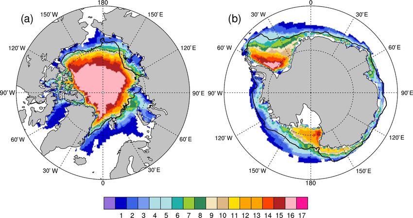
B. L. Otto-Bliesner et al.: Large-scale features of Last Interglacial climate                                                   65

850–1850 CE) and the mid-Pliocene Warm Period (mPWP,               piControl simulations. A new syntheses of surface tempera-
3.3–3.0 × 10⁶ years ago) experiments.                              ture and precipitation proxies, targeted for 127 ka, is used for
   The LIG is recognized as an important period for testing        comparison to the model simulations. We also explore dif-
our knowledge of climate and climate–ice-sheet interactions        ferences in the responses of surface temperature, monsoon
to forcing in warm climate states. Although the LIG was            precipitation, and Arctic sea ice to the different magnitudes
discussed in the First Assessment Report of the IPCC (Fol-         and seasonal character of the insolation anomalies at 127 ka
land et al., 1990), it gained more prominence in the IPCC          versus 6 ka. We then conclude with a discussion of possible
Fourth and Fifth Assessments (AR4 and AR5) (Jansen et al.,         reasons for the model–data differences and implications for
2007; Masson-Delmotte et al., 2013). Evidence in the geo-          future projections.
logic record indicates a warm Arctic (CAPE, 2006; Turney
and Jones, 2010) and a global mean sea level highstand at
                                                                   2     Methods
least 5 m higher (but probably no more than 10 m higher)
than the present for several thousand years during the LIG         2.1    Experimental design
(Dutton et al., 2015). The ensemble of LIG simulations ex-
amined in the AR5 (Masson-Delmotte et al., 2013) was not           The CMIP DECK piControl for 1850 CE (see Eyring et al.,
wholly consistent; the orbital forcing and greenhouse gas          2016, for description of this experiment) is the preindus-
(GHG) concentrations varied between the simulations. While         trial (PI) reference simulation to which the lig127k paleo-
it had been suggested that differences in regional tempera-        experiment is compared. The modeling groups were asked to
tures between models might reflect differences in cryosphere       use the same model components and follow the same proto-
feedback strength (Yin and Berger, 2012; Otto-Bliesner et al.,     cols for implementing external forcings as used in the piCon-
2013) or differences in the simulation of the Atlantic Merid-      trol. The boundary conditions for the lig127k and piControl
ional Overturning Circulation (AMOC) (Bakker et al., 2013),        experiments are described in Otto-Bliesner et al. (2017) and
differences between models could also have arisen because          the Earth System Documentation (2019). More detailed in-
of differences in the experimental protocols. Furthermore,         formation is given below and in Table 1.
the LIG simulations were mostly made with older and/or                 Earth’s orbital parameters (eccentricity, longitude of per-
lower-resolution versions of the models than were used for         ihelion, and obliquity) are prescribed following Berger and
future projections, making it more difficult to use the results    Loutre (1991). The DECK piControl simulations use the or-
to assess model reliability (Lunt et al., 2013).                   bital parameters appropriate for 1850 CE (Table 1, Fig. 1)
   For the first time an LIG experiment is included as a           (Eyring et al., 2016), when perihelion occurs close to the bo-
CMIP6 simulation, setting a common experimental proto-             real winter solstice. The orbit at 127 ka is characterized by
col and asking modeling groups to run with the same model          larger eccentricity than at 1850 CE, with perihelion occur-
and at the same resolution as the DECK simulations (Otto-          ring close to the boreal summer solstice (Table 1, Fig. 1). The
Bliesner et al., 2017). At the PAGES QUIGS workshop in             tilt of the Earth’s axis was maximal at 131 ka and remained
Cambridge in 2015, the community identified the 127 ka             higher than in 1850 CE through 125 ka; obliquity at 127 ka
time slice for the CMIP6–PMIP4 LIG experiment for sev-             was 24.04◦ (Table 1). The solar constant for the lig127k sim-
eral reasons: large Northern Hemisphere seasonal insolation        ulations is prescribed to be the same as in the DECK piCon-
anomalies, no (or little) remnants of the North American and       trol simulation.
Eurasian ice sheets, and sufficient time to allow for dating un-       The orbital parameters affect the seasonal and latitudinal
certainties to minimize the imprint of the previous deglacia-      distribution and magnitude of solar energy received at the
tion and the Heinrich 11 (H11) meltwater event (Marino et          top of the atmosphere, resulting in large positive insolation
al., 2015). The Tier 1 lig127k experiment addresses the cli-       anomalies during boreal summer at 127 ka as compared to
mate responses to stronger orbital forcing, relative to the mid-   1850 CE (Fig. 1). Positive insolation anomalies are present
Holocene. It also provides a basis to address the linkages be-     from April to September and from 60◦ S to 90◦ N. These
tween ice sheets and climate change in collaboration with          anomalies peak at over 70 W m−2 in June at 90◦ N. Insola-
the Ice Sheet Model Intercomparison Project for CMIP6 (IS-         tion in the Arctic (defined here as 60–90◦ N) is more than
MIP6) (Nowicki et al., 2016).                                      10 % greater at 127 ka than 1850 CE during May through
   In this paper, we start with a brief overview of the exper-     early August. The higher obliquity at 127 ka contributes to
imental design of the lig127k (Otto-Bliesner et al., 2017).        a small but positive annual insolation anomaly compared to
We briefly summarize the simulation of temperature, pre-           1850 CE at high latitudes in both hemispheres and negative
cipitation, and sea ice, in the subset of CMIP6 piControl          annual insolation anomaly at tropical latitudes. The global
simulations that have a corresponding lig127k simulation, as       difference in annual insolation forcing between the lig127k
compared to observational datasets. We then provide an ini-        and piControl experiments is negligible.
tial analysis of the multi-model ensemble mean and model               Ice core records from Antarctica provide measurements of
spread in the lig127k surface temperature, precipitation, and      the well-mixed GHGs: CO2 , CH4 , and N2 O. By 127 ka, the
Arctic sea ice responses as compared to the CMIP6 DECK             concentrations of atmospheric CO2 and CH4 had increased

https://doi.org/10.5194/cp-17-63-2021                                                               Clim. Past, 17, 63–94, 2021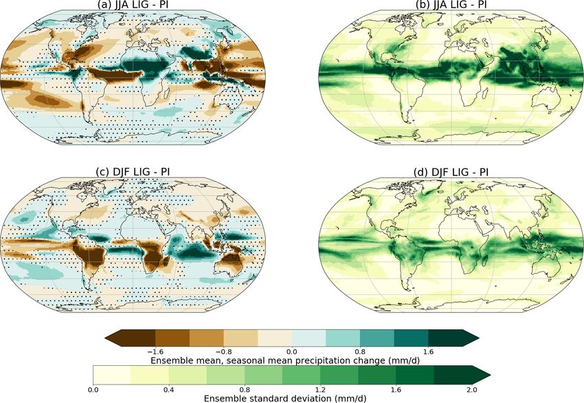
66                                                                B. L. Otto-Bliesner et al.: Large-scale features of Last Interglacial climate

Table 1. Protocols: forcings and boundary conditions.

                                                            1850 CE (DECK piControl)                 127 ka (lig127k)
                 Orbital parameters∗
                 Eccentricity                               0.016764                                 0.039378
                 Obliquity (degrees)                        23.459                                   24.040
                 Perihelion – 180                           100.33                                   275.41
                 Vernal equinox                             Fixed to noon on 21 March                Fixed to noon on 21 March
                 Greenhouse gases
                 Carbon dioxide (ppm)                       284.3                                    275
                 Methane (ppb)                              808.2                                    685
                 Nitrous oxide (ppb)                        273.0                                    255
                 Other GHG gases                            CMIP DECK piControl                      0
                 Solar constant (W m−2 )                    TSI: 1360.747                            Same as piControl
                 Paleogeography                             Modern                                   Same as piControl
                 Ice sheets                                 Modern                                   Same as piControl
                 Vegetation                                 CMIP DECK piControl                      Prescribed or interactive as in piControl
                 Aerosols (dust, volcanic, etc.)            CMIP DECK piControl                      Prescribed or interactive as in piControl
               ∗ The term “orbital parameters” is used to denote the variations in the Earth’s eccentricity and longitude of perihelion as well as changes
               in its axial tilt (obliquity).

Figure 1. (a, b) Orbital configurations for the piControl and lig127k experiments. The number of days between the vernal equinox and
summer solstice, summer solstice and autumnal equinox, etc., are indicated along the periphery of the ellipse. Latitude–month insolation
anomalies 127 ka–1850 in (c) W m−2 and (d) percentage change from PI.

from their minimum levels during the previous glacial pe-                                deMenocal et al., 2000; Kohfeld and Harrison, 2000). Model-
riod to values comparable to, albeit somewhat lower than,                                ing groups were asked to implement changes in atmospheric
preindustrial levels (Table 1).                                                          dust aerosol in their lig127k simulations following the treat-
   Natural aerosols show large variations on glacial–                                    ment used for their DECK piControl simulations (see Table 2
interglacial timescales, with low aerosol loadings during in-                            for details). The background volcanic stratospheric aerosol
terglacials compared to glacials and during the peak of the in-                          used in the CMIP6 DECK piControl was also to be used
terglacials compared to the present day (Albani et al., 2015;                            for the lig127k simulation. Other aerosols included in the

Clim. Past, 17, 63–94, 2021                                                                                            https://doi.org/10.5194/cp-17-63-2021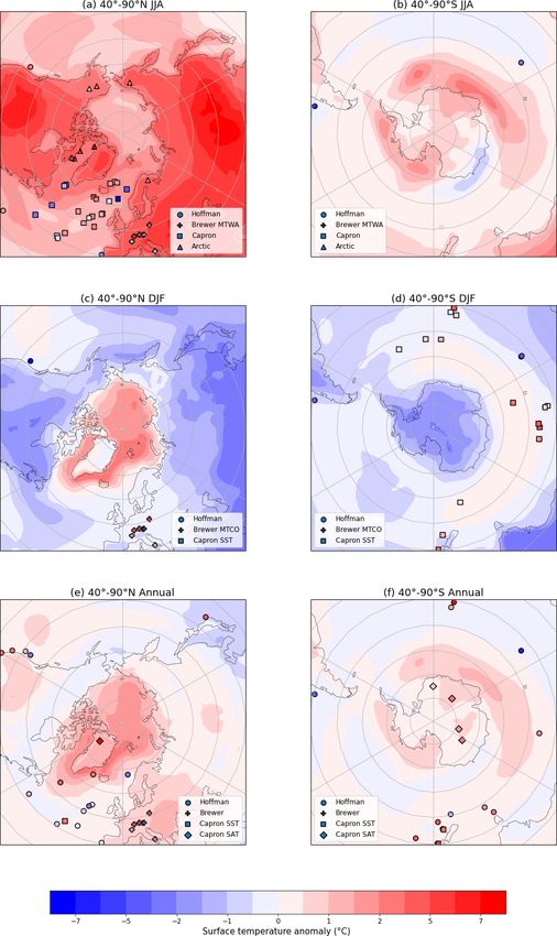
B. L. Otto-Bliesner et al.: Large-scale features of Last Interglacial climate                                                                                          67

Table 2. Summary of CMIP6–PMIP4 models in this intercomparison.

  Climate model                   Institution          Citation for                    Equilibrium (Effective)          Citation for lig127k
                                  name                 model description               climate sensitivity1             experiment and notes2
  ACCESS-ESM1-5                   UNSW and             Ziehn et al. (2017,             3.9 ◦ C                          Yeung et al. (2020); fixed vegetation
                                  CSIRO                2020)                                                            with interactive leaf area index, pre-
                                                                                                                        scribed
                                                                                                                        aerosols
  AWI-ESM-1-1-LR                  AWI                  Sidorenko et al. (2015)         3.1 ◦ C                          Interactive vegetation
  AWI-ESM-2-1-LR                  AWI                  Sidorenko et al. (2019)         3.1 ◦ C                          Interactive vegetation, prescribed
                                                                                                                        aerosols
  CESM2                           NCAR                 Danabasoglu et al.              5.2 ◦ C                          Otto-Bliesner et al. (2020);
                                                       (2020)                                                           prescribed potential vegetation (crops
                                                                                                                        and urban areas removed), interactive
                                                                                                                        phenology, simulated dust
  CNRM-CM6-1                      CNRM-                Voldoire et al. (2019)          4.8 ◦ C                          PI atmospheric GHGs,
                                  CERFACS              Decharme et al. (2019)                                           prescribed vegetation and aerosols
  EC-Earth3-LR                    Stockholm                                            4.2 ◦ C                          Zhang et al. (2020);
                                  University                                                                            prescribed vegetation and aerosols
  FGOALS-f3-L                     CAS                  He et al. (2020)                3.0 ◦ C                          Zheng et al. (2020);
                                                                                                                        prescribed vegetation and aerosols
  FGOALS-g3                       CAS                  Li et al. (2020)                2.8 ◦ C                          Zheng et al. (2020);
                                                                                                                        prescribed vegetation and aerosols
  GISS-E2-1-G                     NASA-GISS            Kelley et al.                   2.7 ◦ C                          –
                                                       (2020)
  HadGEM3-GC31-LL                 BAS                  Kuhlbrodt et al. (2018)         5.6 ◦ C                          Guarino et al. (2020);
                                                       Williams et al. (2017)                                           Williams et al. (2020);
                                                                                                                        prescribed vegetation and aerosols
  INM-CM4-8                       INM RAS              Volodin et al. (2018)           1.8 ◦ C                          Prescribed vegetation,
                                                                                                                        simulated dust and sea salt
  IPSL-CM6A-LR                    IPSL                 Boucher et al. (2020)           4.6 ◦ C                          Prescribed vegetation, interactive
                                                                                                                        phenology, prescribed aerosols
  MIROC-ES2L                      AORI                 Hajima et al. (2020)            2.7 ◦ C                          Ohgaito et al. (2020);
                                  University                                                                            O’ishi et al. (2020);
                                  of                                                                                    prescribed vegetation and aerosols
                                  Tokyo
  MPI-ESM1-2-LR                   AWI                  Giorgetta et al. (2013)         3.0 ◦ C                          Scussolini et al. (2019);
                                  MPI-Met                                                                               interactive vegetation,
                                                                                                                        prescribed aerosols
  NESM3                           NUIST                Cao et al. (2018)               4.7 ◦ C                          Interactive vegetation,
                                                                                                                        prescribed aerosols
  NorESM1-F                       Norwegian            Guo et al. (2019)               2.3 ◦ C                          Prescribed vegetation and aerosols
                                  Climate
                                  Centre, NCC
  NorESM2-LM                      Norwegian            Seland et al. (2020)            2.5 ◦ C                          Prescribed vegetation and aerosols
                                  Climate
                                  Centre, NCC
1 ECS uses the Gregory method from a 150-year run of an instantaneously quadrupled CO simulation (Meehl et al., 2020; Wyser et al., 2020). 2 Unless otherwise noted,
                                                                                     2
prescribed vegetation and aerosols are as in each model’s piControl simulation.

https://doi.org/10.5194/cp-17-63-2021                                                                                               Clim. Past, 17, 63–94, 2021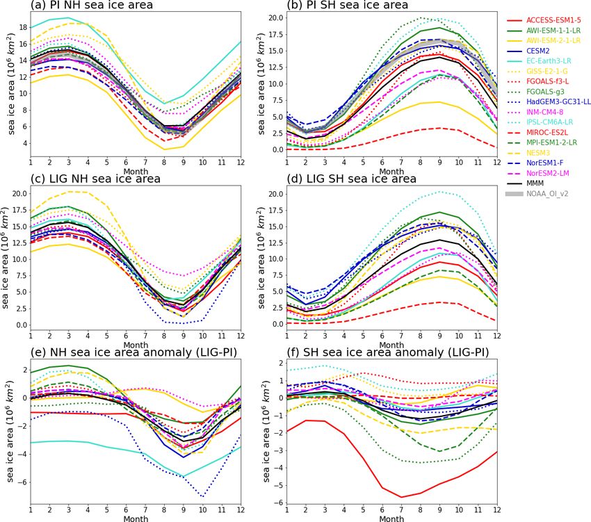
68 B. L. Otto-Bliesner et al.: Large-scale features of Last Interglacial climate
DECK piControl simulations should similarly be included in 3 Simulation results
the lig127k simulations.
There is evidence for changes in vegetation distribution 3.1 Preindustrial simulations
during the LIG (e.g., LIGA Members, 1991; CAPE, 2006;
Larrasoana, 2013). However, there is insufficient data cover- Brierley et al. (2020) provide an extensive evaluation of the
age for many regions to be able to produce reliable global CMIP6 preindustrial simulations as compared to observa-
vegetation maps. Furthermore, given the very different levels tional datasets: reanalyzed climatological temperatures (be-
of complexity in the treatment of vegetation properties in the tween 1871–1900 CE; Compo et al., 2011) for the spatial
current generation of climate models, paleo-observations do patterns, zonal averages of observed temperature for the pe-
not provide sufficient information to constrain their behavior riod 1850–1900 CE from the HadCRUT4 dataset (Morice et
in a comparable way. The treatment of natural vegetation in al., 2012; Ilyas et al., 2017), and climatological precipitation
the lig127k simulations was therefore to be the same as in data for the period between 1970 and the present day (Adler
the DECK piControl simulation. Accordingly, depending on et al., 2003). In summary, they find that the PMIP4–CMIP6
what was done in the DECK piControl simulation, vegetation models are in general cooler than the observations, most no-
could either be prescribed to be the same as in that simula- ticeably at the poles, over land, and over the NH oceans. The
tion, prescribed but with interactive phenology, or predicted poleward extent of the North African monsoon, in particular,
dynamically (see Table 2 for implementations in the models). is underestimated in the CMIP6 preindustrial simulations.
Paleogeography and ice sheets were to be kept at their The CMIP6 midHolocene and lig127k have 14 models in
present-day configuration. common (see Fig. 4a in Brierley et al., 2020, and Fig. 2a in
this paper). The piControl multi-model mean (MMM), zonal-
2.2 Model evaluation average temperature is slightly cooler than observed at high
(60–90◦ N) Northern Hemisphere (NH) latitudes (Fig. 2a).
The 17 modeling groups that have completed CMIP6 lig127k There is a large spread across the models though, with eight
simulations are presented in this paper (Table 2). All used the of the models simulating colder (up to 4 ◦ C) than observed
CMIP6 version of their model also used for their DECK ex- temperatures and nine of the models simulating warmer (up
periments. The equilibrium climate sensitivity (ECS) varies to 2 ◦ C) than observed temperatures. The piControl MMM,
from 1.8 to 5.6 ◦ C. The years analyzed for each model and zonal-average temperature is noticeably warmer than ob-
DOIs for each of the simulations are given in Table S1 in the served at high (60–90◦ S) Southern Hemisphere (SH) lati-
Supplement. The analysis uses data available on the CMIP6 tudes, again with a large spread across the models. Two mod-
ESGF (Earth System Grid Federation) for surface air tem- els – MIROC-ES2L and EC-Earth3-LR – have biases in ex-
perature (tas), precipitation (pr), and sea ice concentration cess of 5 ◦ C. Hajima et al. (2020) attribute the MIROC-ES2L
(siconc). piControl warm bias over the Southern Ocean to it being
mainly associated with the model’s representation of cloud
2.3 Calendar adjustments radiative processes. The spread of the piControl simulations
is smaller at low and midlatitudes (Fig. 2a).
The output is corrected following Bartlein and Shafer (2019),
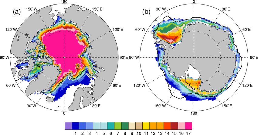
We adopt the definition of sea ice area of the Sea Ice
to account for the impact that the changes in the length of
Model Intercomparison Project (SIMIP; SIMIP Community,
months or seasons over time have on the analysis (Fig. 1).
2020), i.e., sea ice concentration times the cell area. The
This correction is necessary to account for the impact of the
multi-model ensemble of piControl simulations of minimum
changes in the eccentricity of the Earth’s orbit and the pre-
(August–September) Arctic sea ice distribution (Figs. 3a,
cession when using the “celestial” calendar. Not consider-
S2) show good agreement with the 15 % contour from the
ing the “paleo-calendar effect” can prevent the correct inter-
HadISST data averaged over the 1870–1920 period (Fig. S1)
pretation of data and model comparisons at 127 ka, with the
(Rayner et al., 2003). Two models – FGOALS-g3 and EC-
largest problems occurring in boreal fall/austral spring (Jous-
Earth3-LR – show noticeably greater minimum summer sea
saume and Braconnot, 1997; Bartlein and Shafer, 2019). A
ice extent in the Nordic Seas as compared to the HadISST
more detailed discussion of the application of the PaleoCal-
period (Fig. S2). Further, evaluation of the piControl simu-
Adjust software to past time periods with strong orbital forc-
lations can be found in Kageyama et al. (2021). In partic-
ing can be found in Bartlein and Shafer (2019) and Brierley
ular, they find that in comparison to sea ice reconstruction
et al. (2020).
sites, the models generally overestimated sea ice cover at
sites close to the sea ice edge.
Figure 4 shows the seasonal cycle of Arctic sea ice area
in the piControl simulations for each model and the MMM.
These are compared to the NOAA OI_v2 observational
dataset, with higher temporal and spatial coverage than the
HadISST dataset. The NOAA_OI_v2 dataset (Reynolds et
Clim. Past, 17, 63–94, 2021 https://doi.org/10.5194/cp-17-63-2021
B. L. Otto-Bliesner et al.: Large-scale features of Last Interglacial climate                                                            69

Figure 2. (a) Comparison of the preindustrial zonal mean temperature profile of individual climate models and MMM to the 1850–1900
observations. The area-averaged, annual mean surface air temperature for 30◦ latitude bands in the CMIP6 models and a spatially complete
compilation of instrumental observations over 1850–1900 (black; Ilyas et al., 2017; Morice et al., 2012). (b) Changes in zonal average, mean
annual surface air temperatures (lig127k minus piControl).

al., 2002), also used in Kageyama et al. (2021), only extends           tica, however, show less consensus among the models
back to 1981. It should be noted that atmospheric CO2 con-              and less agreement with the HadISST data, with many
centrations had already risen to 340 ppm by 1981, as com-               models significantly underestimating the observed austral
pared to 284.7 ppm specified in the piControl simulations.              summer minimal extent (Figs. 3b, 4b, S4). The range
We find a large spread across the piControl simulations. The            in February is 0.02 to 3.82 × 10⁶ km2 and the MMM is
range in March is 12.27 to 19.16 × 10⁶ km2 and the MMM                  1.65 ± 1.21 × 10⁶ km2 . Antarctic sea ice melts back largely
is 15.30 ± 1.89 × 10⁶ km2 . The range in September is 3.56              to the continent’s edge in February–March in four mod-
to 9.73 × 10⁶ km2 , and the MMM is 6.13 ± 1.66 × 10⁶ km2 .              els (AWI-ESM-2-1-LR, EC-Earth3-LR, MIROC-ES2L, and
Generally, those models with less sea ice in March than the             MPI-ESM1-2-LR) (Fig. S5). The spread of models is even
MMM also have less sea ice in September than the MMM.                   greater in their simulations of piControl austral winter sea
Observed estimates of sea ice area from the NOAA-OI_v2                  ice area around Antarctica, ranging from 3.27 × 10⁶ km2
dataset for 1982–2001 are 14.7 × 10⁶ km2 for March and                  in September in MIROC-ES2L to over 19 × 106 km2 in
5.1 × 10⁶ km2 for September.                                            IPSL-CM6-LR and FGOALS-g3. The September MMM
   The MMM piControl simulations of austral summer min-                 is 17.13 ± 5.21 × 10⁶ km2 . Observed estimates of sea ice
imum (February–March) sea ice distribution around Antarc-               area from the NOAA-OI_v2 dataset for 1982–2001 are

https://doi.org/10.5194/cp-17-63-2021                                                                      Clim. Past, 17, 63–94, 2021
70 B. L. Otto-Bliesner et al.: Large-scale features of Last Interglacial climate
Figure 3. Comparison of the piControl sea ice distributions (a) in the Northern Hemisphere for August–September and (b) in the Southern
Hemisphere for February–March. For each 1◦ × 1◦ longitude–latitude grid cell, the figure indicates the number of models that simulate at
least 15 % of the area covered by sea ice. The observed 15 % concentration boundaries (black lines) are the 1870–1919 CE interval based on
the Hadley Centre Sea Ice and Sea Surface Temperature (HadISST; Rayner et al., 2003) dataset. See Figs. S2 and S4 for individual model
results.
2.7 × 10⁶ km2 for February and 16.5 × 10⁶ km2 for Septem- In response to the negative insolation anomalies at all lat-
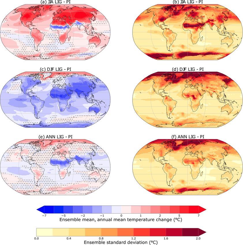
ber. itudes (Fig. 1), the lig127k MMM simulates cooling during
DJF over the continental regions of both hemispheres and
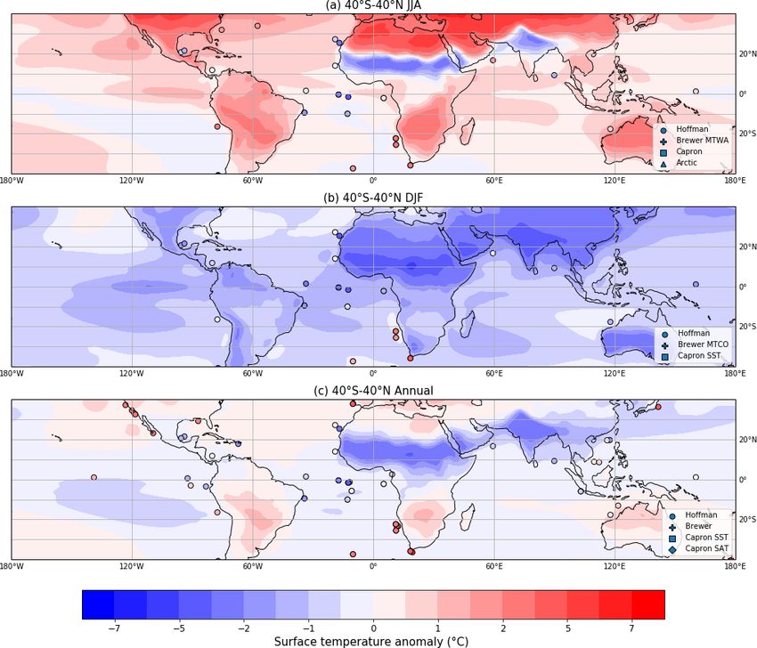
3.2 Surface temperature responses low and midlatitude oceans (Fig. 5c). The largest DJF tem-
perature anomalies occur over southeastern Asia and north-
The seasonal character of the insolation anomalies results in ern Africa. Ocean memory has been shown to provide the
warming and cooling over the continents in the lig127k en- feedback to maintain positive or neutral DJF temperature
semble (relative to the piControl) in June–July–August (JJA) anomalies in the Arctic and North Atlantic (see Serreze and
and December–January–February (DJF), respectively, except Barry, 2011, for further discussion). As indicated by the stan-
for the African and southeast Asian monsoon regions in JJA. dard deviations of the ensemble changes, large differences in
These patterns of seasonal, continental warming and cooling the magnitude of the DJF high-latitude, surface temperature
are a robust feature across the models, with more than 70 % responses and feedbacks exist among the models (Fig. 5d).
of the models agreeing on the sign of the temperature change Understanding these differences warrants further analyses in
(Fig. 5a, c). future studies.
The warming during JJA is greater than 6 ◦ C at midlat- These seasonal patterns of change are similar to those
itudes in North America and Eurasia (Fig. 5a), though with found in Lunt et al. (2013), though the warming is larger in
significant differences in the magnitude of the warming in the the CMIP6 simulations. It should be noted that the MMM
southeast US, Europe, and eastern Asia among the models in Lunt et al. (2013) includes simulations that have varying
(Fig. 5b). Further investigation of the effects of preindustrial orbital years (between 125 and 130 ka) and greenhouse gas
vegetation, including crops, for these regions in the lig127k concentrations.
protocol would be useful (Otto-Bliesner et al., 2020). Sub- Annually, the MMM surface temperature changes between
tropical land areas in the Southern Hemisphere (SH) also re- the lig127k and piControl are generally less than 1 ◦ C over
spond to the positive (but more muted) insolation anomalies, most of the globe, with two exceptions (Fig. 5e): greater neg-
with JJA temperature anomalies more than 2 ◦ C warmer than ative surface temperature anomalies across the North African
PI. JJA warming over most of the oceans is a robust feature and Indian monsoon regions and positive surface tempera-
across the models. This warming is greatest in the North At- ture anomalies in the Arctic. Although more than 70 % of the
lantic and the Southern Ocean, though with large differences models agree on the sign of the changes in these regions, as
across the ensemble of models (Fig. 5b). Cooling over the well as in the Indian sector of the Southern Ocean (Fig. 5e),
Sahel and southern India in JJA is associated with the in- the across-ensemble standard deviations indicate differences
creased cloud cover associated with the enhanced monsoons in the magnitudes of the annual surface temperature re-
(see Sect. 3.4). sponses (Fig. 5f). Globally, the MMM change in annual sur-
face air temperature is close to zero (−0.2 ± 0.32 ◦ C), though
Clim. Past, 17, 63–94, 2021 https://doi.org/10.5194/cp-17-63-2021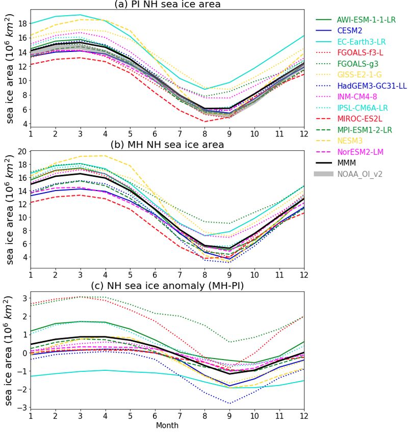
B. L. Otto-Bliesner et al.: Large-scale features of Last Interglacial climate                                                           71

Figure 4. The simulated Arctic (a, c, e) and Antarctic (b, d, f) annual cycle of sea ice area (106 km2 ) for the (a, b) PI, (c, d) LIG, and
(e, f) LIG minus PI. The monthly mean sea ice areas from the NOAA_OI_v2 dataset for 1982–2001 (Reynolds et al., 2002) are shown in
panels (a) and (b).

with a large spread among the models (−0.48 to 0.56 ◦ C) (Ta-           FGOALS-f3-L are cooler in their lig127k simulations as
ble 3). Conclusions about the land versus ocean or NH versus            compared to their piControl simulations. The spread (and
SH annual temperatures changes are complicated by mean                  magnitude) of mean annual temperature change for the SH
changes being close to zero and not consistently positive or            polar region is less, with 7 of 17 models simulating a mod-
negative (Table 3).                                                     est warming of 0–1 ◦ C and 3 models simulating a cool-
   The large spread of mean annual surface temperature                  ing of the mean annual surface temperature (Fig. 2b). The
change among the models in the polar regions (60–90◦ lat-               MMM is 0.38 ± 0.63 ◦ C. The change in the NH latitudinal
itude) is further illustrated in Fig. 2b. Annual Arctic surface         gradient is positive from all models: 1.27 ◦ C in the MMM
temperature changes in the lig127k simulations range from               though ranging quite significantly among models for 0.30 ◦ C
−0.39 to 3.88 ◦ C. The MMM is 0.82 ± 1.20 ◦ C. Notably,                 in FGOALS-f3-L and 3.94 ◦ C in EC-Earth3-LR (Table 3).
EC-Earth3-LR and HadGEM3-GC3.1-LL have anomalies                        The change in the SH latitudinal gradient is smaller (0.47 ◦ C
greater than 3 ◦ C in their lig127k simulations as compared             in the MMM), reflecting the prescription of a modern Antarc-
to their piControl simulations, while AWI-ESM-1-1-LR and                tic ice sheet in the lig127k experiment (Table 3). Changes in

https://doi.org/10.5194/cp-17-63-2021                                                                     Clim. Past, 17, 63–94, 2021
72                                                     B. L. Otto-Bliesner et al.: Large-scale features of Last Interglacial climate

Figure 5. Multi-model ensemble average changes (a, c, e) and across-ensemble standard deviations (b, d, f) of surface air temperatures (◦ C)
for lig127k minus piControl. Shown are June–July–August (a, b), December–January–February (c, d), and annual mean (e, f) changes. Dots
indicate where less than 12 (70 %) of the 17 models agree on the sign of the change.

the size of the Antarctic ice sheet during the Last Interglacial        sea ice area. HadGEM3-GC31-ll simulates an ice-free Arctic
would be expected to result in warming at polar latitudes in            in August–September–October, with the largest reduction in
the SH and an increase in the SH latitudinal gradient (Bradley          October (Fig. 4c, e). EC-Earth3-LR has the largest reduction
et al., 2012; Otto-Bliesner et al., 2013; Stone et al., 2016)           of March sea ice area for lig127k as compared to its piCon-
                                                                        trol, and AWI-ESM2-1-LR has a notable increase (Fig. 4e).
                                                                        As shown also in Kageyama et al. (2021), PI biases in simu-
3.3   Sea ice responses                                                 lation of the minimum Arctic sea ice are not always a good
                                                                        predictor of reductions at lig127k (Fig. 4c).
Boreal insolation anomalies at 127 ka enhance the seasonal
                                                                           The individual model lig127k minimum (August–
cycle of Arctic sea ice (Fig. 4c). There is a ∼ 50 % re-
                                                                        September) Arctic sea ice area anomalies show negative cor-
duction and shift of minimum area in the MMM from
                                                                        relations (−0.65) with the Arctic (60–90◦ N) annual sur-
6.1 × 10⁶ km2 in August–September for PI to 3.1 × 10⁶ km2
                                                                        face temperature anomalies from their respective piControl
in September for lig127k, with a range of 0.22 to
                                                                        simulations and negative correlation (−0.53) with the cor-
7.47 × 10⁶ km2 in the individual lig127k simulations. The
                                                                        responding JJA temperature anomalies, both significant at
lig127k MMM maximum winter sea ice area in the Arctic
                                                                        the 0.05 significance level (Fig. 7). Memory in the ocean
in March is 15.68 ± 2.08 × 10⁶ km2 with a range of 12.27
                                                                        and cryosphere memory provide feedbacks to maintain pos-
to 20.28 × 10⁶ km2 . The INM-CM4-8 and AWI-ESM2-1-LR
                                                                        itive temperature anomalies, DJF and annually, in the Arc-
have small reductions in sea ice area in all seasons with
                                                                        tic (Fig. 5). Analyzing the summer atmospheric heat budgets
the largest decrease in October (Fig. 4e). HadGEM3-G31-ll
                                                                        across the models, Kageyama et al. (2021) find that the dif-
and EC-Earth3-LR have large reductions in minimum Arctic

Clim. Past, 17, 63–94, 2021                                                                    https://doi.org/10.5194/cp-17-63-2021
B. L. Otto-Bliesner et al.: Large-scale features of Last Interglacial climate 73
Table 3. Metrics for surface air temperature change (◦ C) for CMIP6–PMIP4 lig127k simulations.
Climate Model Global Global Global NH NH NH SH SH SH NH SH
land ocean land ocean land ocean meridional meridional
gradient1 gradient2
ACCESS-ESM1-5 0.33 0.42 0.29 0.43 0.34 0.48 0.23 0.58 −0.05 1.61 1.89
AWI-ESM-1-1-LR −0.25 −0.47 −0.16 −0.55 −0.81 −0.37 0.04 0.25 −0.08 0.38 0.86
AWI-ESM-2-1-LR −0.20 −0.34 −0.14 −0.39 −0.59 −0.25 −0.01 0.20 −0.14 0.8 0.78
CESM2 −0.11 −0.16 −0.09 −0.22 −0.31 −0.16 0.00 0.18 −0.08 1.02 0.47
CNRM-CM6-1 0.4 0.39 0.4 0.33 0.15 0.46 0.46 0.89 0.26 1.21 0.55
EC-Earth3-LR 0.45 0.71 0.34 0.99 0.92 1.03 −0.07 0.32 −0.17 3.94 0
FGOALS-f3-L −0.48 −0.57 −0.44 −0.60 −0.77 −0.48 −0.37 −0.16 −0.35 0.3 −0.28
FGOALS-g3 0.38 0.6 0.29 0.38 0.51 0.29 0.48 0.89 0.24 2.42 1.14
GISS-E2-1-G −0.12 −0.1 −0.13 −0.07 −0.17 0.00 −0.18 0.06 −0.20 1.59 −0.11
HadGEM3-GC31-LL 0.56 0.71 0.49 0.89 0.76 0.97 0.22 0.62 0.08 3.08 0.37
INM-CM4-8 −0.2 −0.3 −0.15 −0.30 −0.54 −0.14 −0.09 0.20 −0.12 0.45 −0.23
IPSL-CM6A-LR −0.29 −0.3 −0.29 −0.29 −0.43 −0.19 −0.30 −0.03 −0.31 0.89 −0.02
MIROC-ES2L −0.4 −0.55 −0.33 −0.52 −0.73 −0.38 −0.26 −0.12 −0.29 0.92 0.55
MPI-ESM1-2-LR −0.12 −0.24 −0.07 −0.33 −0.54 −0.19 0.10 0.42 −0.05 0.95 0.83
NESM3 0.07 −0.02 0.11 −0.25 −0.43 −0.12 0.39 0.86 0.22 0.83 0.57
NorESM1-F −0.24 −0.35 −0.2 −0.33 −0.55 −0.18 −0.15 0.08 −0.21 0.59 0.24
NorESM2-LM −0.11 −0.04 −0.14 −0.13 −0.13 −0.12 −0.09 0.16 −0.16 0.69 0.39
Mean −0.02 −0.04 −0.01 −0.06 −0.20 0.04 0.02 0.32 −0.08 1.27 0.47
SD 0.32 0.44 0.28 0.48 0.54 0.45 0.26 0.34 0.19 1.00 0.55
Max 0.56 0.71 0.49 0.99 0.92 1.03 0.48 0.89 0.26 3.94 1.89
Min −0.48 −0.57 −0.44 −0.60 −0.81 −0.48 −0.37 −0.16 −0.35 0.30 −0.28
1 60–90◦ N minus 0–30◦ N. 2 60–90◦ S minus 0–30◦ S.
ferent Arctic sea ice responses can be related to the sea ice 1.84 ± 1.42 × 10⁶ km2 (Fig. 4d). This is similar to the MMM
albedo feedback, i.e., phasing of the downward solar insola- of the piControl simulations (Fig. 4b). In both the lig127k
tion changes associated with the orbital forcing and reflected and piControl, the models exhibit widely different sea ice
upward shortwave flux changes associated with the sea ice areas (0.06 to 4.65 × 10⁶ km2 ) and distributions for the aus-
cover changes. As has been done for evaluating simulations tral summer (Fig. S5). Those models that simulate summer
of present sea ice distributions, it would be useful for further sea ice in the Weddell Sea in the piControl (Fig. S4) retain
studies to also explore model differences in the simulated this sea ice in their lig127k simulation. The maximum austral
changes in high-latitude cloudiness, boundary layer, winds, winter sea ice around Antarctica also varies widely among
and ocean processes (Kattsov and Källén, 2005; Arzel et al., the models, with the MIROC-ES2L simulating the smallest
2006; Chapman and Walsh, 2007). area (and seasonal cycle) and IPSLCM6 simulating the high-
Previous studies suggest that the mean-ice state in the con- est areal extent (and seasonal cycle) (Fig. 4b, d) in the pi-
trol climate can influence the magnitude and spatial distribu- Control and lig127k simulations. ACCESS-ESM1-5 has the
tion of warming in the Arctic in future projections (Holland greatest sensitivity to the lig127k forcings (Fig. 4f).
and Bitz, 2003). Thinner Arctic sea ice is more susceptible The consensus from the lig127k sea ice distributions is a
to summer melting than thicker Arctic sea ice. Arctic sea reduced minimum (August–September) summer sea ice ex-
ice thickness varies substantially across the 1850 CE ensem- tent (defined as 15 % concentration) in the Arctic (Fig. 6) as
ble, ranging from 1–1.5 m in CNRM-CM6-1 and NESM3 to compared to the piControl simulations (Fig. 3). It is interest-
∼ 7.5 m in MIROC-ES2L (not shown). No robust relation- ing to compare the MMM simulated summer sea ice extents
ship to the August–September lig127k minimum Arctic sea in the lig127k simulations to the observed sea ice extents
ice area anomaly is present. This is also true for the CMIP6– for 2000–2018 (black lines in Fig. 6). More than half of the
PMIP4 mid Holocene simulations (Brierley et al., 2020). One models simulate a retreat of the Arctic minimum (August–
reason for a lack of any relationship may be the seasonal na- September) ice edge at 127 ka, similar to the average of
ture of the lig127k and midHolocene insolation forcings as the last 2 decades. The pattern of February–March Southern
compared to the annual forcing by greenhouse gas changes Ocean sea ice extent is broadly similar in the lig127k simu-
in future projections. lations to 2000–2018, though four models simulate a larger
The lig127k austral summer sea ice around Antarc- sea ice area.
tica has a minimum in February in the MMM of
https://doi.org/10.5194/cp-17-63-2021 Clim. Past, 17, 63–94, 202174 B. L. Otto-Bliesner et al.: Large-scale features of Last Interglacial climate
Figure 6. Comparison of the lig127k sea ice distributions (a) in the Northern Hemisphere for August–September and (b) in the Southern
Hemisphere for February–March. For each 1◦ × 1◦ longitude–latitude grid cell, the figure indicates the number of models that simulate at
least 15 % of the area covered by sea ice. The average 15 % concentration boundaries (black lines) are averaged for 2000–2018. See Figs. S3
and S5 for individual model results.
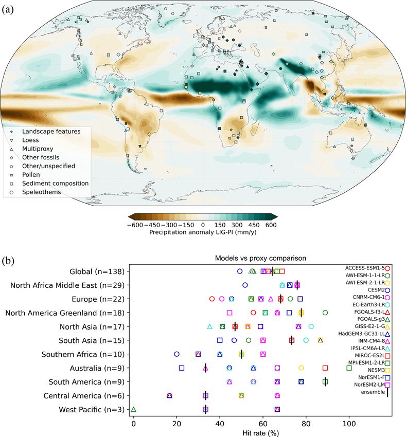
3.4 Precipitation responses
The seasonal character of the insolation anomalies results
in enhanced summer monsoonal precipitation in the lig127k
ensemble (relative to the piControl ensemble) over north-
ern Africa, extending into Saudi Arabia, India and south-
east Asia, and northwestern Mexico/the southwestern US
(Fig. 8a). In contrast, summer monsoonal precipitation de-
creases over South America, southern Africa, and Australia.
The spread among models is large, however, as shown by the
across-ensemble standard deviations (Fig. 8b, d) and percent-
age changes in area-averaged precipitation during the mon-
soon season for seven different regional monsoon domains
for the individual lig127k simulations (Fig. 16a). The mod-
els generally agree on the sign of the percentage changes
in the area-averaged precipitation rate during the monsoon
season for the monsoon regions, except for the East Asian,
South Asian, and Australian–Maritime Continent monsoons
where some models simulate increased monsoonal precipita-
tion whereas others show decreases.
Over the tropical Pacific Ocean, reduced DJF precipitation
over the Intertropical Convergence Zone (ITCZ) is a robust
feature across the ensemble of lig127k simulations (Fig. 8c).
The models simulate a shift of the tropical Atlantic ITCZ
Figure 7. (a) lig127k August–September sea ice NH area anomaly northward in JJA and southward in DJF, though with signifi-
(106 km2 ) versus lig127k annual 60–90◦ N surface air tempera- cant differences among the models of the ensemble (Fig. 8a,
ture anomaly (◦ C); (b) lig127k August–September NH sea ice area b). Over the Indian Ocean, the ensemble mean indicates more
anomaly (106 km2 ) versus lig127k JJA 60–90◦ N surface air tem- precipitation in DJF over the entire basin and less in JJA, par-
perature anomaly (◦ C). ticularly in the central and eastern basin, though again with
large standard deviations (Fig. 8).
Figure 9 shows the ensemble-averaged lig127k change in
monsoon-related rainfall rate and global monsoon domain.
Increases in the summer rainfall rate and areal extent of the
Clim. Past, 17, 63–94, 2021 https://doi.org/10.5194/cp-17-63-2021B. L. Otto-Bliesner et al.: Large-scale features of Last Interglacial climate 75 Figure 8. Multi-model ensemble average changes (a, c) and across-ensemble standard deviations (b, d) of precipitation (mm d−1 ) for lig127k minus piControl. Shown are June–July–August (a, b) and December–January–February (c, d) changes. Dots indicate where less than 12 (70 %) of the 17 models agree on the sign of the change. Figure 9. Ensemble-averaged Last Interglacial change in monsoon-related rainfall rate (in mm d−1 ). Red and blue contours show the bound- aries of lig127k and piControl monsoon domains, respectively, using the definitions of Wang et al. (2011). North Africa and East Asia monsoon are clear and are ro- cipitated in each monsoon season varying from ∼ 70 %– bust across the multi-model ensemble. The spread across 140 % (Fig. 16c). The models are in closer agreement for the multi-model ensemble is considerable, though, for the the East Asian monsoon (EAS), with the percentage change North African (NAF) monsoon, with the percentage change in the areal extent varying from ∼ 10 %–35 % (Fig. 16b) and in the areal extent varying from ∼ 40 %–120 % (Fig. 16b) the percentage change in the total amount of water precip- and the percentage change in the total amount of water pre- itated in each monsoon season varying from ∼ 25 %–40 % https://doi.org/10.5194/cp-17-63-2021 Clim. Past, 17, 63–94, 2021
76                                                B. L. Otto-Bliesner et al.: Large-scale features of Last Interglacial climate

(Fig. 16c). The lig127k and piControl simulations produce        variations observed in independently dated Asian speleothem
more muted changes for the other monsoon regions in the          records (Speleo-Age) (Barker et al., 2011) in the compila-
MMM, with regards to the regional monsoon-related rain-          tion by Hoffman et al. (2017). Note that the two reference
fall rate and the monsoon domains (Fig. 9). Four models          chronologies diverge by about 1 kyr at 127 ka (Capron et al.,
(AWI-ESM-1-1-LR, AWI-ESM-2-1-LR, MPI-ESM1-2-LR,                  2017).
NESM3) in the lig127k ensemble include interactive vege-            The two compilations then follow quite similar Monte
tation. Even then, these four models generally fall within the   Carlo approaches to propagate temperature and chronolog-
spread of the models with prescribed vegetation for the three    ical uncertainties. Indeed, both compilations generate 1000
metrics and seven monsoon regions (Fig. 16).                     realizations of the site-specific surface temperature records
                                                                 to integrate the uncertainty in the temperature reconstruc-
                                                                 tion’s method, and both produce 1000 possible chronologies
4     Data reconstructions
                                                                 to propagate the relative age uncertainty related to alignment
4.1    Marine temperatures
                                                                 of records. For a given site, the temperature at 127 ka is the
                                                                 temperature value directly taken at 127 ka in the compilation
The lig127k climate model simulations are assessed using         by Hoffman et al. (2017), using dated temperature time se-
two complementary compilations of sea surface tempera-           ries interpolated every 1 kyr. In the compilation of Capron et
ture (SST) anomalies at 127 ka (Tables S3–S5, S7), which         al. (2014, 2017), the temperature at 127 ka is taken as the
are both individually based on stratigraphically consistent      median temperature averaged over the 128–126 ka period.
chronologies (Capron et al., 2017; Hoffman et al., 2017).        Finally, temperature anomalies relative to the preindustrial
   The multi-archive high-latitude compilation by Capron         period are calculated in both cases for marine sites using
et al. (2014, 2017) includes 42 sea surface annual/summer        the HadISST dataset (Rayner et al., 2003), over the inter-
temperature records with a minimum temporal resolution of        vals 1870–1899 and 1870–1889 CE, in the compilations by
2 kyr for latitudes above 40◦ N and 40◦ S, along with five ice   Capron et al. (2017) and Hoffman et al. (2017), respectively.
core surface air temperature records. In contrast, the global    For both compilations, the provided 2σ uncertainties inte-
marine compilation by Hoffman et al. (2017) includes 186         grate errors linked to relative dating and surface temperature
annual, summer, and winter SST records from the Atlantic,        reconstruction methods.
Indian, and Pacific oceans, with a minimum temporal resolu-         Nevertheless, because of (1) the different reference
tion of 4 kyr on their published age models. Note that, in ad-   chronologies used, (2) the different tie points and associ-
dition to the annual microfossil assemblage SST records cal-     ated relative age uncertainties defined to derive the chronol-
culated for 41 sites as the average of the summer and winter     ogy of each site, and (3) the different calculation methods
records with a model- and observation-consistent correction      (Bayesian statistics versus linear interpolation between tie
for annual offsets (Hoffman et al., 2017), we also provide       points) used in the Monte Carlo age model analysis of each
here for these specific sites the updated seasonal (summer       site (despite apparently relatively similar approaches), the
and winter) SST estimates on the Hoffman et al. (2017) age       two compilations by Capron et al. (2014, 2017) and by Hoff-
models. SSTs from marine cores are reconstructed in both         man et al. (2017) are listed as such in Tables S2–S5, S7. Im-
compilations from foraminiferal Mg/Ca ratios, alkenone un-       plications of these methodological differences in the inferred
saturation ratios or microfossil faunal assemblage transfer      127 ka values are best illustrated when comparing the sur-
functions (Capron et al., 2014, 2017; Hoffman et al., 2017).     face temperature time series deduced from the two different
   To derive the LIG marine chronologies, both compila-          approaches for a same North Atlantic (62◦ N) site: at 127 ka,
tions make use of the climate-model-supported hypothesis         a temperature offset of ∼ 2 ◦ C is observed between the two
that surface-water temperature changes in the sub-Antarctic      reconstructions (see Fig. 4 of Capron et al., 2017).
zone of the Southern Ocean (respectively in the North At-
lantic) occurred simultaneously with air temperature varia-      4.2   Ice core temperatures
tions above Antarctica (respectively Greenland) (Capron et
al., 2014; Hoffman et al., 2017). The compilation by Hoff-       Surface air temperature records for one site (NEEM) on the
man et al. (2017) then uses basin-synchronous LIG changes        Greenland ice sheet and four sites on the Antarctic ice sheet
in the oxygen isotopic composition of benthic foraminifera,      are deduced from ice core water isotopic profiles (Capron
as observed in previous studies of benthic foraminiferal         et al., 2014, 2017) (Tables S2 and S4). For ice cores, prein-
isotope changes across glacial terminations (Lisiecki and        dustrial conditions are estimated using borehole temperature
Raymo, 2009) within the same ocean basins, to align intra-       measurements for Greenland and 1870–1899 CE water iso-
basin chronologies. However, a major difference is the un-       topic profiles for Antarctica (Capron et al., 2017). Tempera-
derlying reference chronology used in both compilations: the     tures are again the median for the 126–128 ka period and are
Antarctic Ice Core Chronology 2012 (AICC2012) (Bazin et          considered to represent annual averages. Uncertainty is esti-
al., 2013; Veres et al., 2013) in the compilation by Capron et   mated using the same Monte Carlo procedure as was used for
al. (2014, 2017) and a chronology based on millennial-scale      the marine cores in the compilation of Capron et al. (2017).

Clim. Past, 17, 63–94, 2021                                                           https://doi.org/10.5194/cp-17-63-2021
B. L. Otto-Bliesner et al.: Large-scale features of Last Interglacial climate 77
Because it uses the same reference timescale (AICC2012), time t (Brewer et al., 2008). Here we present the mean value
the ice core dataset can be considered coherent with the ma- and standard deviation for mean annual temperature, mean
rine SST dataset of Capron et al. (2017). temperature of the coldest month, and mean temperature of
the warmest month across all sites for 127 ka.
4.3 Terrestrial temperatures
Of the 15 terrestrial sites used by Brewer et al. (2008), 8
were excluded due to uncertainties over their chronostrati-
Calibrated, well-dated reconstructions of Last Interglacial graphical or chronological assignments or because they did
temperatures over the continents are quite limited. We have not extend to 127 ka.
assembled two distinct compilations of continental air tem- The Arctic dataset compiles the most stratigraphically
perature reconstructions: a dataset of air temperatures over complete, best time-constrained, and calibrated summer tem-
Europe at 127 ka based on Brewer et al. (2008) and a compi- perature reconstructions published from above 65◦ N lati-
lation of peak Last Interglacial summer temperatures recon- tude. We report the mean of the two warmest consecutive
structed at Arctic sites from pollen and insect assemblages reconstructions at each site, utilizing the original published
(Table S6). For both we report anomalies comparing recon- models and reconstructions. For sites where both insect-
structed temperatures with preindustrial climate estimated and pollen-based temperature reconstructions have been pub-
from 1871–1900. lished or where multiple models have been applied to the
In Europe, favorable geological conditions have led to the same proxy, we report here the average of those reconstruc-
accumulation of numerous LIG sediment sequences from a tions. We report the original published model uncertainties
variety of depositional environments (Tzedakis, 2007). These (e.g., root mean square error of prediction for weighted av-
include former kettle lakes overlying late Saalian (MIS 6) eraging models), including the most conservative (largest)
till, depressions left by the penultimate alpine glaciation or model uncertainties for sites where multiple proxies/models
local ice caps, and volcanic crater lakes or tectonic grabens are applied. This differs from error reporting for the Eu-
mainly in the unglaciated south. Over several decades, a sub- ropean dataset above. Importantly, the Arctic compilation
stantial body of pollen evidence has provided an insight into also differs from the other paleotemperature datasets used
the LIG vegetational development across Europe. A number here, in that it reports the warmest LIG conditions regis-
of pollen-based climate reconstructions based on reference tered at each site rather than temperatures at 127 ka. This ap-
sequences have been attempted, using a variety of methods. proach was necessitated by the coarse temporal resolutions
However, differences between underlying assumptions and and chronologies of the North American Arctic reconstruc-
data employed (e.g., taxon presence–absence versus abun- tions, which come from stratigraphically discontinuous de-
dance) mean that results have been difficult to compare. posits dated by 14 C (non-finite 14 C ages) and in some cases
Here, we include data from one study that has applied a luminescence or tephrochronology. In contrast to the North
multi-method approach to assess combined uncertainties of American Arctic sites, in northern Finland (Sokli) and north-
reconstruction and age models on a set of reference pollen east Russia (El’gygytgyn) correlative dating provides contin-
records (Brewer et al., 2008). The reconstruction methods uous chronologies. The reported peak warmth at those sites
used are (i) partial least squares, (ii) weighted average par- occurred at ∼ 125 and 127–125 ka, respectively (Melles et
tial least squares, (ii) generalized additive models, (iv) artifi- al., 2012; Salonen et al., 2018). Reconstructed temperature at
cial neural network, (v) unweighted modern analogue tech- Sokli at 127 ka was ∼ 1 ◦ C lower than the peak temperature
nique, (vi) weighted modern analogue technique, and (vii) re- reported here from that site. The Greenland ice-core-derived
vised analogue method using response surfaces. Timescales temperature reconstruction from NEEM complements the
for the pollen sequences were developed by transferring the Arctic terrestrial dataset, but it reflects annual rather than
marine chronology to land sequences for certain pollen strati- summer-specific climate.
graphical events on the basis of joint pollen and paleoceano- Despite an abundance of LIG pollen records from Eura-
graphic analyses in deep-sea sequences on the Portuguese sia and various attempts at pollen-based climate reconstruc-
Margin and Bay of Biscay (Shackleton et al., 2003; Sánchez tions (e.g., compilations Velichko et al., 2008; Turney and
Goñi et al., 2008). With particular reference to constraining Jones, 2010), chronological and methodological uncertain-
the 127 ka time slice, the pollen stratigraphical events used ties continue to complicate comparisons with climate model
were the onset of the Quercus (128.8 ± 1 ka) and Carpinus outputs. The lack of spatial coherence in the European tem-
(124.77 ± 1 ka) expansions (Brewer et al., 2008). For each perature reconstructions may reflect depth–age model issues
site, chronological uncertainties were estimated at each sam- at individual sites, which implies that the 127 ka time slice
ple by randomly sampling an age from the range around each had not been correctly identified. An alternative approach
control point, fitting a linearly interpolated age model and would have been to select peak temperatures from a wider
repeating this 1000 times (Brewer et al., 2008). Reconstruc- interval (e.g., 127 ± 2 ka) and assume that these are quasi-
tions were made at 500-year intervals by randomly sampling synchronous. In addition, the Arctic reconstruction may be
within the chronological uncertainties and reconstruction er- skewed towards warmer temperatures than the models, given
rors for each method, resulting in 1400 estimates for each
https://doi.org/10.5194/cp-17-63-2021 Clim. Past, 17, 63–94, 2021You can also read