The response of the corona to different spatial distributions of heat input
←
→
Page content transcription
If your browser does not render page correctly, please read the page content below
The response of the corona to different
  spatial distributions of heat input

                           Dissertation
zur Erlangung des mathematisch-naturwissenschaftlichen Doktorgrades

                    “Doctor rerum naturalium”

              der Georg-August-Universität Göttingen

                im Promotionsprogramm PROPHYS
      der Georg-August University School of Science (GAUSS)

                           vorgelegt von
                     Tijmen van Wettum
                 aus Nieuwegein / The Netherlands

                         Göttingen, 2013
Betreuungsausschuss

Prof. Hardi Peter
Max-Planck-Institut für Sonnensystemforschung, Göttingen, Germany

Prof. Jens Niemeyer
Institut für Astrophysik, Georg-August-Universität Göttingen, Germany

Mitglieder der Prüfungskommision

Referent: Prof. Hardi Peter
Max-Planck-Institut für Sonnensystemforschung, Göttingen, Germany

Korreferent: Prof. Jens Niemeyer
Institut für Astrophysik, Georg-August-Universität Göttingen, Germany

Weitere Mitglieder der Prüfungskommission:

Prof. Dr. Manfred Schüssler
Max-Planck-Institut für Sonnensystemforschung, Göttingen, Germany

Prof. Dr. Laurent Gizon
Max-Planck-Institut für Sonnensystemforschung, Göttingen, Germany

Prof. Dr. Ansgar Reiners
Max-Planck-Institut für Sonnensystemforschung, Göttingen, Germany

Prof Dr. Ulrich R. Christensen
Max-Planck-Institut für Sonnensystemforschung, Göttingen, Germany

Tag der mündlichen Prüfung: 26. 09. 2013
Bibliografische Information der Deutschen Nationalbibliothek
Die Deutsche Nationalbibliothek verzeichnet diese Publikation in der
Deutschen Nationalbibliografie; detaillierte bibliografische Daten
sind im Internet über http://dnb.d-nb.de abrufbar.

ISBN 978-3-942171-76-2

uni-edition GmbH 2013
http://www.uni-edition.de
c Tijmen van Wettum
          This work is distributed under a
          Creative Commons Attribution 3.0 License

Printed in Germany

                                                                       3
Contents

Summary                                                                                                                                 9

1   Introduction                                                                                                                       11
    1.1 Our central star . . . . . . . . . . . . . . . . . . . . . . . . . . . . . . .                                                 11
    1.2 Solar atmosphere . . . . . . . . . . . . . . . . . . . . . . . . . . . . . .                                                   12

2   Motivation                                                                                                                         15
    2.1 The hot Corona . . . . . . . .     .   .   .   .   .   .   .   .   .   .   .   .   .   .   .   .   .   .   .   .   .   .   .   15
    2.2 Coronal energy budget . . . .      .   .   .   .   .   .   .   .   .   .   .   .   .   .   .   .   .   .   .   .   .   .   .   16
    2.3 Heating mechanisms . . . . .       .   .   .   .   .   .   .   .   .   .   .   .   .   .   .   .   .   .   .   .   .   .   .   17
         2.3.1 AC heating . . . . . .      .   .   .   .   .   .   .   .   .   .   .   .   .   .   .   .   .   .   .   .   .   .   .   17
         2.3.2 DC heating . . . . . .      .   .   .   .   .   .   .   .   .   .   .   .   .   .   .   .   .   .   .   .   .   .   .   18
         2.3.3 No consensus . . . . .      .   .   .   .   .   .   .   .   .   .   .   .   .   .   .   .   .   .   .   .   .   .   .   19
    2.4 Modelling of the Solar corona      .   .   .   .   .   .   .   .   .   .   .   .   .   .   .   .   .   .   .   .   .   .   .   19
         2.4.1 1D models . . . . . .       .   .   .   .   .   .   .   .   .   .   .   .   .   .   .   .   .   .   .   .   .   .   .   19
         2.4.2 3D coronal box models       .   .   .   .   .   .   .   .   .   .   .   .   .   .   .   .   .   .   .   .   .   .   .   20
         2.4.3 Dopplershifts . . . . .     .   .   .   .   .   .   .   .   .   .   .   .   .   .   .   .   .   .   .   .   .   .   .   21
    2.5 Motivation for present study .     .   .   .   .   .   .   .   .   .   .   .   .   .   .   .   .   .   .   .   .   .   .   .   22

3   Magneto Hydro-Dynamics                                                                                                             23
    3.1 Maxwell Equations . . . . . . . . . . . . . .                      .   .   .   .   .   .   .   .   .   .   .   .   .   .   .   23
    3.2 Ohm’s law . . . . . . . . . . . . . . . . . . .                    .   .   .   .   .   .   .   .   .   .   .   .   .   .   .   24
    3.3 MHD equations . . . . . . . . . . . . . . . .                      .   .   .   .   .   .   .   .   .   .   .   .   .   .   .   25
        3.3.1 Continuity equation . . . . . . . . . .                      .   .   .   .   .   .   .   .   .   .   .   .   .   .   .   25
        3.3.2 Equation of motion . . . . . . . . . .                       .   .   .   .   .   .   .   .   .   .   .   .   .   .   .   26
        3.3.3 Energy equation . . . . . . . . . . .                        .   .   .   .   .   .   .   .   .   .   .   .   .   .   .   27
        3.3.4 Induction equation . . . . . . . . . .                       .   .   .   .   .   .   .   .   .   .   .   .   .   .   .   30
    3.4 Vector Potential . . . . . . . . . . . . . . . .                   .   .   .   .   .   .   .   .   .   .   .   .   .   .   .   31
    3.5 Ordering of plasma along the magnetic field. .                     .   .   .   .   .   .   .   .   .   .   .   .   .   .   .   31
    3.6 Poynting flux . . . . . . . . . . . . . . . . .                    .   .   .   .   .   .   .   .   .   .   .   .   .   .   .   32
    3.7 The flow of energy in the model . . . . . . .                      .   .   .   .   .   .   .   .   .   .   .   .   .   .   .   32

4   Treatment of model corona                                                                                                          35
    4.1 Model philosophy . . . . . . . . . . . . . . . . . . . . . . . . . . . . . .                                                   35
    4.2 Numerical scheme used by the Pencil Code . . . . . . . . . . . . . . . .                                                       35
         Time step . . . . . . . . . . . . . . . . . . . . . . . . . . . . . . . . . .                                                 36

                                                                                                                                       5
Contents
4.3 Implementation of the MHD equations . . . . . . . . . . . . . . . . . . . 36
Coronal module . . . . . . . . . . . . . . . . . . . . . . . . . . . . . . . 37
4.4 Numerical model setup . . . . . . . . . . . . . . . . . . . . . . . . . . . 38
4.4.1 Boundary conditions . . . . . . . . . . . . . . . . . . . . . . . . 38
4.4.2 Initial conditions . . . . . . . . . . . . . . . . . . . . . . . . . . 39
4.5 Heating parametrizations . . . . . . . . . . . . . . . . . . . . . . . . . . 40
4.5.1 Ohmic heating in the model . . . . . . . . . . . . . . . . . . . . 41
4.5.2 Alfvénic heating . . . . . . . . . . . . . . . . . . . . . . . . . . 41
4.5.3 MHD turbulence . . . . . . . . . . . . . . . . . . . . . . . . . . 42
4.6 Synthetic emission . . . . . . . . . . . . . . . . . . . . . . . . . . . . . 42
4.7 Mean atomic weight . . . . . . . . . . . . . . . . . . . . . . . . . . . . 43
4.8 Extraction of field-lines . . . . . . . . . . . . . . . . . . . . . . . . . . . 45
5 Heating along individual fieldlines 47
5.1 Goal . . . . . . . . . . . . . . . . . . . . . . . . . . . . . . . . . . . . . 47
5.2 Method . . . . . . . . . . . . . . . . . . . . . . . . . . . . . . . . . . . 47
5.2.1 Horizontal averages . . . . . . . . . . . . . . . . . . . . . . . . . 47
5.2.2 Heating along individual field-lines . . . . . . . . . . . . . . . . 49
5.2.3 The “random set” of field-lines . . . . . . . . . . . . . . . . . . . 51
5.2.4 From field-lines to loop models . . . . . . . . . . . . . . . . . . 53
5.3 Details of 1D coronal models . . . . . . . . . . . . . . . . . . . . . . . . 54
5.4 One-dimensional coronal loop models . . . . . . . . . . . . . . . . . . . 55
5.5 Conclusions . . . . . . . . . . . . . . . . . . . . . . . . . . . . . . . . . 58
6 Coronal heat input and magnetic activity 61
6.1 Goal . . . . . . . . . . . . . . . . . . . . . . . . . . . . . . . . . . . . . 61
6.2 Method . . . . . . . . . . . . . . . . . . . . . . . . . . . . . . . . . . . 62
6.3 Results . . . . . . . . . . . . . . . . . . . . . . . . . . . . . . . . . . . . 62
6.3.1 Heating in time . . . . . . . . . . . . . . . . . . . . . . . . . . . 63
6.3.2 Doppler shifts . . . . . . . . . . . . . . . . . . . . . . . . . . . . 68
6.3.3 Flux flux relation . . . . . . . . . . . . . . . . . . . . . . . . . . 68
6.4 Conclusion & Discussion . . . . . . . . . . . . . . . . . . . . . . . . . . 71
7 Testing parametrizations of coronal heating 73
7.1 Goal . . . . . . . . . . . . . . . . . . . . . . . . . . . . . . . . . . . . . 73
7.2 Model set-up . . . . . . . . . . . . . . . . . . . . . . . . . . . . . . . . 73
7.3 Results . . . . . . . . . . . . . . . . . . . . . . . . . . . . . . . . . . . . 74
7.3.1 Emission . . . . . . . . . . . . . . . . . . . . . . . . . . . . . . 78
7.3.2 Doppler shifts . . . . . . . . . . . . . . . . . . . . . . . . . . . . 78
7.3.3 Direct comparison of heat input for parametrizations . . . . . . . 79
7.4 Discussion and conclusion . . . . . . . . . . . . . . . . . . . . . . . . . 80
8 Discusion and conclusion 85
8.1 Conclusion . . . . . . . . . . . . . . . . . . . . . . . . . . . . . . . . . 85
8.2 Outlook . . . . . . . . . . . . . . . . . . . . . . . . . . . . . . . . . . . 86
Bibliography 87
6Contents
Publications 93
Acknowledgements 95
Curriculum Vitae 97
7Summary
Explaining the existence of the million degree corona on top of the much cooler Solar
surface has provided scientist with a challenge for a several decades. It is not possible for
a cooler object to heat something that is hotter by conduction, which implies that there is
another mean of energy transport into the corona. The general consensus is that this role
is taken by the magnetic fields that are ever present at the solar surface.
The focus of today’s research is on the actual mechanism that thermalizes the energy
transported by the magnetic field. Several mechanisms responsible for this conversion
into thermal energy are being put forward. These suggestions fall often in the Alternating
Current (AC) or Direct Current (DC) category. The first involves rapid changes of the
magnetic field relative to the Alfvén crossing time of a coronal loop, while the second
category involves slow changes. While a convincing case can be made for each suggested
heating mechanism from modelling alone, the observational confirmation is lacking. The
theoretical estimates on which scales the energy conversion happens in these models,
are on the order of centimetres to metres. Observations, however, reach a resolution of
100 km, at best, in the relevant wavelengths, and as such no direct observational confir-
mation of one heating mechanism over the other is possible.
Synthetic observations derived from self-consistent 3D MHD models can provide the link
between theory and observation. Investigation of the emission structures and distribution
of Doppler shifts of emission lines can provide insight on which of these mechanisms is
dominant. Fully self consistent 3D MHD models have already shown the feasibility of
this method. In this work we will expand this approach in two ways.
First we investigate the effect of the strength of the magnetic field at the photospheric
layer. We find that the behaviour of the Doppler shifts is strongly depended on the the
magnetic field strength. When interpreting the stronger photospheric magnetic fields as
higher magnetic activity, the patterns seen in the Doppler shifts as a function of formation
temperature are consistent with observation of magnetically active stars. Also comparing
the C IV emission with a proxy for the X-ray flux is roughly consistent with observations.
Next we explore the observational consequences of different heating mechanisms using
3D MHD numerical experiments. This provides some insight on which of these mech-
anisms is dominant. For this we replace the Ohmic heating term in the energy equation
with parametrized forms of the heating, which are derived from reduced MHD models.
These models involve heating through Alfvén wave dissipation and MHD-turbulence. We
find that the different heating parametrizations give similar coronae in terms of synthe-
sized emission as it would be observed e.g. by EUV imaging. Thus EUV imaging alone
are not sufficient to distinguish between these parametrizations. However, Doppler shift
observations acquired by e.g. Hinode/EIS can provide the pivotal information. In our
numerical experiments the different parametrizations of the heating leads to significantly
9Summary different distributions of the Doppler shifts of the synthesized emission lines in the tran- sition region and corona. In particular, this applies to the average redshifts seen in the transition region and the average blueshifts in the coronal lines. Based on this, our results favour the turbulent cascade over the Alfvén wave heating, at least when considering an active region. Future observational and numerical studies will have to show to what ex- tend this will hold in general. Combining the results from the two investigations we conclude that different heating dis- tributions produce different observables. But it is not trivial to conclude which distribution is the most likely. 10
1 Introduction

1.1     Our central star
The Sun has always played an important role in history, religion and science. Almost ev-
ery religion had major role for the Sun god of goddess. The occurrence of a solar eclipse
was often seen as a bad sign, and in many civilizations it was thought the Sun was being
eaten by a giant monster. Therefore the prediction of such an event was considered of ut-
ter importance. As such the Chinese civilization was able to predict these already around
2000 BCE. The Greeks followed around 600 BCE. This is very impressive considering
their ignorance on the nature of the cosmos. Around this time Chinese records mention
the appearance of a darkening or obscuration on the solar disk. These are now understood
to be sunspots.
The Dutch invention of the telescope in the beginning of the seventeenth century allowed
for systematic recording of Sun spots. These recordings are still used today to reconstruct
past solar activity. Some of the most well-known records of the sunspots are those by
Galileo. The number of spots on the Sun follows a cycle of roughly eleven years. This
was only found in the middle of the 19th century by a German astronomer Samuel Hein-
rich Schwabe. It might have been discovered as earlier as in the time of Galileo, if it
were not for the peculiar behaviour of the Sun at that time. From roughly 1600 until 1750
nearly no sunspots appeared on the surface, and the solar cycle seemed to have stopped.
Nowadays we know that the solar cycle is actually a 22 year cycle. In this cycle the
magnetic North and South pole of the sun reverses and back again. During a solar min-
imum the Solar magnetic field is close to a dipole, but during a reversal the magnetic
field becomes very chaotic. At this time strong patches of magnetic flux emerge from the
solar surface. The strongest of those are able to push away the plasma and inhibit convec-
tion, making these areas show up as cool, dark patches on the solar surface, e.g. sun spots.

Core

The energy radiated away by the Sun surface originates from the core. In this region the
temperature reaches well over 15 million degrees and together with the high pressure this
is enough to fuse hydrogen into helium. The small difference in mass between these two
atoms, is released as energy in the form of radiation and neutrinos. The latter provided the
pivotal evidence that the process of nuclear fusion actually occurred in the Sun. Before
that time it was thought the Sun was powered predominantly through the energy released
by the gravitational contraction. This would however not agree with the age found for

                                                                                         11
1 Introduction the Earth and evolution to occur. The gravity powered Sun would have an estimated life- time of roughly 10 million years, whereas the age of the earth was estimated to be of the order of 5 billion years. The detection of the Solar neutrinos confirmed fusion takes place in the core, and the age of the Sun shifted to 5 billion years. It is expected the that our star can be powered by fusion for another 5 billion years before the hydrogen runs out. Radiative zone It has been estimated that a photon (in the classic sense) remains between a hundred thou- sand and one million years inside the Sun. During this time the photon is scattered around by free electrons. This constant scattering provides a significant amount of pressure, as well as an important means of energy transport. In the radiative zone, just above the core, this is the dominant energy transport mechanism. If one would fall into the Sun, and not burn instantly, only halfway radiative zone you would come to a rest. At this point the density equals that of a human body, i.e. water. Convective zone In the convective zone this mode of energy transfer changes. Convective motion takes over from radiation at roughly 86% of the Solar radius as the most efficient way of energy transport. Bubbles of hot plasma rise up from the tachocline, the interface between the radiative and the convective zone. From there the bubbles of hot plasma move upward toward the solar surface. There energy is lost trough radiation. After cooling the cold plasma sinks back into the solar interior. This is what we observe as granular motion on the surface. 1.2 Solar atmosphere The Solar atmosphere is separated in three different zones, distinguished by their different physical properties. Photosphere In this layer the most of the energy from the Sun is lost through radiation. The temper- ature at the bottom of the photosphere is 6600 K and drops further to 4300 K at the top. Not all radiation is lost directly from the photosphere, radiation in certain wavelengths are again absorbed by the upper photosphere which holds most of the observed absorp- tion lines. The photospheric energy distribution characterizes the Solar spectrum which follows roughly a 6000 K Planck curve. Chromosphere The Chromosphere is named after its colourful appearance during a solar eclipse. The chromosphere is characterized by a rise in temperature, which is a result of acoustic waves dissipating. The chromosphere is very non-uniform, a view at the limbs sees this region 12
1.2 Solar atmosphere
as a mass of spicules, or mottles as they are called on-disk, which are small jets of plasma.
In contrast to the absorption-dominated photosphere the spectrum of the chromosphere is
emission dominated, mainly as a result of the increasing temperatures. The temperatures
in the chromosphere reach about 10,000 K.
Corona
The interface between the chromosphere and corona is the Transition Region (TR) in
which is characterized by a sudden increase of temperature by several orders of mag-
nitude. Here the temperature of the solar atmosphere surges from tens of thousands of
degrees to over several million degrees.
The first mention of the solar corona was by the Byzantine historian Leo Diaconus, who
mentioned a "dim and feeble glow like a narrow band shining in a circle around the
edge of the disk" around the darkened Sun during the 968 eclipse in Constantinople. The
corona is usually very faint and therefore only visible if the light of the Sun itself blocked,
as is the case during a Solar eclipse. The low intensities are a result of the extremely
low densities. Despite the clearly visible corona during an eclipse, the densities are lower
than the best vacuum we can create on Earth. Modern observatories use a small occulter
to block out the bright solar disk, or observe in high energy wavelengths in which the rest
of the Solar atmosphere is not emitting.
The corona is where magnetic fields have free play and are not prohibited by the dense
plasma as in the chromosphere and photosphere. This leads to coronal loops, bright loops-
like structures of plasma captured by the strong magnetic fields. Also prominences, cooler
and denser plasma hoovering above the solar surface, kept up by magnetic fields. The
magnetic fields lie at the source of extremely violent explosions, solar flares, which set
off coronal mass ejection. These launch plasma from the solar surface into the interplan-
etary space, and if it hits Earth would be able to knock out satellites or even power plants
on the surface. The extreme conditions the plasma is subject to in the corona is unique
and unreproducible in laboratory conditions. Studying the corona is therefore crucial to
fully understand the properties of plasma, the stuff where 99% of our universe is made of.
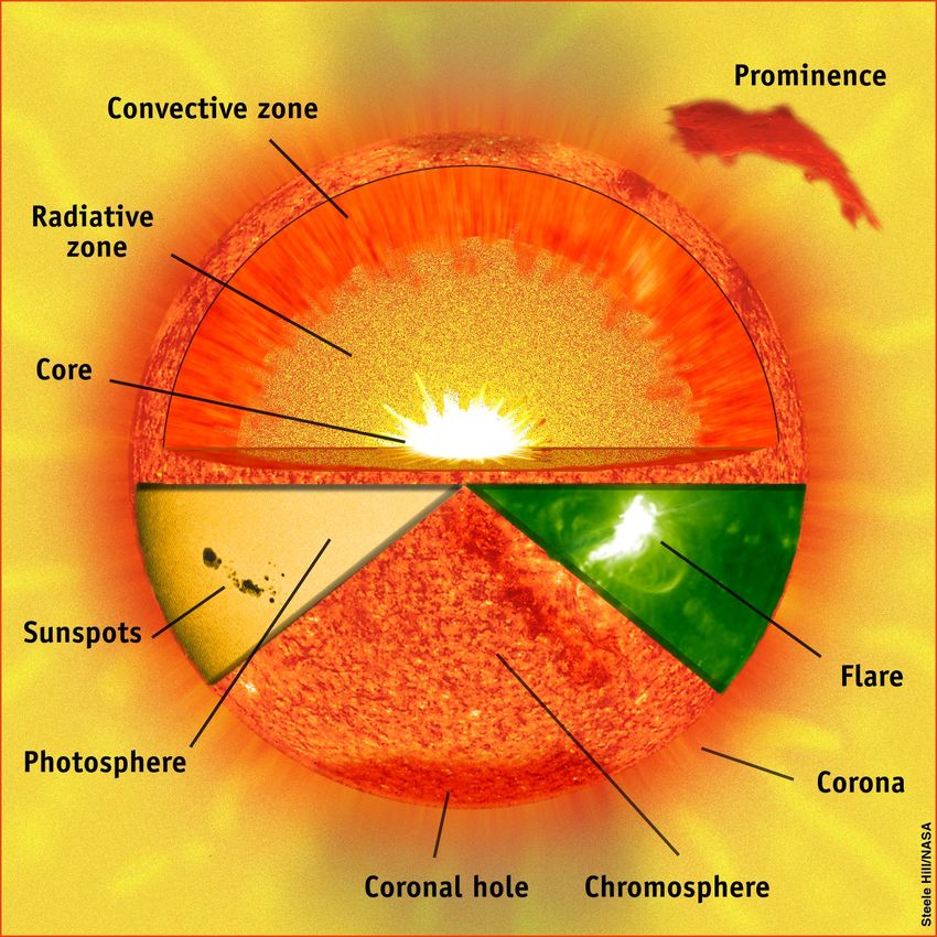
131 Introduction Figure 1.1: A cartoon depicting the different regions of the Sun. Image courtesy of SOHO consortium. SOHO is a project of international cooperation between ESA and NASA. 14
2 Motivation

In this chapter we discuss the context and motivation of our model. This is done by
introducing the coronal heating problem, and discussing the proposed solutions. Next we
give an overview on the current state of numerical models in this field and how our work
fits within.

2.1     The hot Corona
The nature of the corona has been a mystery for a very long time. Several anomalous
observations made this region hard to physically explain. The first to suggest the mil-
lion degree solar corona was Hannes Alfvén in 1941 (Alfvén 1941). This conclusion
was reached after examination of several of these anomalous observations. So was the
energy distribution of the continuum spectrum observed in the corona the same as the
photosphere. This would imply that the light from the photosphere was scatter off free
electrons in the corona.
This was supported by the near absence of the Fraunhofer (absorption) lines, scattering
on a distribution of high velocity electrons would wash out most of these lines, through
the wide distribution of Doppler shifts. Only remnants of the strongest absorption lines
could be observed, such as H and K absorption lines from singly ionized calcium, as was
discovered by Grotrian (1931). The degree of "washing out" is a measure of the mean
electron velocity, and thus the temperature of the coronal electrons. This way the author
found a mean electron velocity of 7.5 · 108 cm s−1 and later 4 · 108 cm s−1 (Grotrian 1934),
which would correspond to temperatures of respectively 1.2 · 106 and 0.35 · 106 degrees.
The existence of so-called "forbidden lines" was observed by Edlén (1943) to whom the
discovery of the million degree corona is usually attributed to. These lines belong to
atoms with an extremely high degree of ionization, such as Fe XIV and Ca XV. To reach
these levels of ionization through collisions would require very high electron energies.
These lines are called "forbidden" because of their relatively low change of spontaneous
de-excitation, which allows the ion to stay in an exited state for a long time. In higher den-
sities the collisional de-excitation rates are therefore much higher than the spontaneous
ones. The coronal densities are however very low, so that the collisions are so infrequent
as to allow the spontaneous (radiative) de-excitation of these excited states. The existence
of these highly ionized atoms, as well as the degree of Doppler broadening of the emis-
sion lines, would require temperatures of the order of a million degrees.
These, and several other lines of evidence, led to the conclusion that the corona actually
is one million degrees and over. Something that was not expected at that time. This dis-
covery led to a new question, "How is the corona heated?", which, in a slightly modified

                                                                                           15
2 Motivation
version, remains one of the greatest unanswered questions in physics.
2.2 Coronal energy budget
The temperature of the corona is remarkably robust. If we think of a simplified picture
of a coronal loop in equilibrium, with energy being deposited in the corona, a majority of
this energy is transported downward though heat conduction and subsequently lost in the
chromosphere through radiation. Scaling laws of coronal temperature and pressure based
on this principle were derived as the RTV-scaling laws (Rosner et al. 1978), who found
these as a result of early 1D models. They developed an order-of-magnitude estimate on
how the apex temperature of a coronal loop scales with the energy input. When assuming
all energy is transported downward and is lost there predominantly through radiation, we
can construct a energy-balance equation
Lrad ≈ ∇ · q ≈ H (2.2.1)
where, the radiative losses, Lrad ∝ ρ2 T α , are a function of the density ρ and temperature
T . α is a result of approximating the radiative losses by a piecewise power law. This is of
the same order as the second term, the energy conduction, which is given by q ∝ T 5/2 ∇T .
This term is again of the same order as the energy input, H. We ignore here all the
constants since our interest lies in how the terms scale with each other, not the absolute
values. The full equations, including the constants are discussed in chapter 3.
The values of α are approximated by −1/2, which provides a good fit over the range of
105 K to 107 K. We know that for a classical gas ρ ∝ p/T , where we take the pressure p
to be constant along the loop. Estimating ∇ with the loop length 1/L, leads to two scaling
laws:
T top ∝ H 2/7 L4/7 , (2.2.2)
p ∝ H 6/7 L5/7 . (2.2.3)
These laws relate the temperature are the top of the loop, T top and the pressure, p, with the
heating rate and loop length. The first scaling law shows that the temperature of a coronal
loop is rather insensitive to the energy input. In order to double the coronal temperature,
one needs to increase the energy input by more than a factor 10.
The coronal heating problem becomes apparent when considering the lower lying and
cooler photosphere. The heating requires an upward non-thermal transport of energy
through the lower cooler regions and a mechanism to deposit this energy into the corona.
To balance the energy losses of the corona trough radiation, particle acceleration and con-
duction, requires an energy flux of 3 · 102 Watt m−2 , for the quiet sun, to 104 Watt m−2 in
active regions (Withbroe and Noyes 1977).
The magnetic fields that are ever present on the Sun provide both the means of energy
transport and more than enough energy to keep the corona at one million degrees As-
chwanden (2004). There is, however, no consensus in what way the magnetic energy is
converted into thermal energy.
162.3 Heating mechanisms
2.3 Heating mechanisms
It is clear from various observations that the heating of the corona is closely linked to
the magnetic field. Strong enhancements in emission lines originating from hot plasma,
coincide with regions of strong magnetic field. This puts the magnetic field at the forefront
as the dominant energy carrier. This is reassuring, since acoustic waves are extremely
inefficient in crossing the transition region. The drop in density in the TR causes these
wave to shock and dissipate well before they reach the corona. Waves in the magnetic field
can travel partially into the corona and deliver sufficient energy across the TR. Changes in
the configuration of the field travel nearly unhindered through the transition region. Also
this allows the transport of sufficient energy Aschwanden (2004) into the corona. The
exact nature of this transport, and subsequent dissipation is still largely unknown. There
are however, many suggestions which general fall within either of the two categories,
alternating current (AC) heating and direct current (DC) heating. This depends on the
time scales involved in respect to the time needed for an Alfvén wave to travel the across
the whole loop.
2.3.1 AC heating
AC heating is characterized by fast changes in the magnetic field configuration, faster
than the field line can adapt to the changing conditions. These fast changes often take
the form of Alfvén waves which are exited by the convective motion at the solar sur-
face. The downflows in the inter-granular lanes are highly turbulent (Cattaneo et al. 2003;
Vögler et al. 2005; Stein and Nordlund 2006; Bushby et al. 2008) and as such causes
transverse motions within the flux elements. A fraction of these waves reach the corona
were, through some mechanism, they dissipate and convert the magnetic energy into ther-
mal.
These Alfvén waves, a pure magnetic wave, have no density perturbation associated with
it, and are therefore hard to detect. Tomczyk et al. (2007) reported the first observations
of these waves using the high temporal and spatial resolution of the AIA instrument on
SDO.
A problem with AC heating based on Alfvén waves is the strong increase of the Alfvén
speed that increases from 15 km s−1 in the photosphere to over 1000 km s−1 in the corona.
This leads, just as for sound waves, to a barrier. The strong reflection of the Alfvén waves
allows only a small fraction of the energy to be transported into into the corona. Due to
the low densities in the corona this leakage of energy through the TR should be sufficient
to heat the corona. The biggest obstacle for these suggestions it that Alfvén waves are
notoriously hard to dissipate because of the independence on the local density.
It is suggested that field-lines in resonance have unique eigen-frequencies. When two
neighbouring field-lines resonate out-of-phase, strong currents that form as a result of this
could dissipate the wave energy and heat the loop (Ionson 1978). Also resonances of
Alfvén waves with ions would deposit sufficient energy Aschwanden (2004). An attrac-
tive feature of the last suggestion is that it also work in open field-lines, and the deposited
energy would not only be sufficient to heat the corona but also to accelerate the solar wind.
172 Motivation
[h]
Figure 2.1: A schematic depiction of field line braiding. The cartoon depicts an unfolded
loop. Photospheric motions entangle the different field-lines. Stress induced by this en-
tanglement is released through reconnection events, which converts magnetic energy into
thermal and kinetic energy. Image taken from Parker (1983)
2.3.2 DC heating
DC heating involves slowly changing magnetic fields, so that the fields can adapt to the
changing conditions. These changes are thought to be induced by the granular motion of
the photosphere that shuffles the magnetic fields around. In the photosphere the thermal
pressure is stronger than the magnetic pressure and as such the magnetic field is forced
to follow the granular flows. In the corona the field-lines are braided which induces
currents which then dissipate and heat the corona. This model was first suggested by
Parker (1972). This is schematically drawn in figure 2.1. In this model the energy is not
continuously released, but will start when enough stress has been accumulated through
the entangling of the magnetic field by photospheric motions. At a critical angle two
braided magnetic field-lines will reconnect and release their stored energy as a short burst
of energy. These short burst of energy are also named "nanoflares" after their relative
strength in comparison to large scale flares.
The dissipation of magnetic energy in these models is thought of to occur through small
scale reconnection events. This change in connectivity of field-lines induces a sudden
contraction of field-lines, similar to letting go of a stretched rubber band. This causes an
acceleration of the charged particles, which then collide with other particles, and in this
way thermalizes the particle flow.
182.4 Modelling of the Solar corona
2.3.3 No consensus
The actual dissipation in both categories would happen on scales of well below metres,
whereas the highest resolution observations reach down to roughly a hundred kilometres.
Therefore all hypotheses for the heating mechanism eventually have to rely on indirect
observations of the heating as the means of confirmation or falsification. It is expected that
different rates and locations of heating lead to different dynamics of the corona, these can
then be used as a probe to give a clue about the underlying mechanism. These observables
can be Doppler shifts as a function of temperature, or the emission structure along a
coronal loop.
It is, however, not trivial to conclude from the various observables the most likely heating
mechanism. This is a result of the chaotic nature of the corona. Heating will cause a
response of the plasma as a result of a change in the pressure balance, which in turn
will change the radiative structure and subsequently influences the different observables
available to us.
Large scale 3D magneto hydrodynamic (MHD) simulations are able to bridge the gap
from heating to observables, but are limited by the same limitation as observations, the
length-scales on which the energy conversion acts. Therefore these models have to fall
back on parametrizations of the heating. Despite this limitation, the models are able
to treat the heating self-consistently in time and space. Therefore realistic large scale
simulations provide the link between theory and observation.
This is where this work makes a contribution. In changing the way the corona is heated,
we hope to produce different structures and dynamics. These can then be used to derive
several statistics that might give a hint on whether these heating mechanisms are feasible.
2.4 Modelling of the Solar corona
This subsection gives a short overview about the modelling done on the coronal heating
problem and the corona in general. This is based on Peter (2007).
2.4.1 1D models
The first models developed to investigate the heating of closed coronal loops were one di-
mensional models. The 1D approach was required because of the limited computational
power at that time, but such an approximation of a coronal loop is none-the-less a good
simplification. Since the plasma is frozen-in into the magnetic field, nearly no flow across
the magnetic field is allowed. The flow of plasma and the energy transport take place
almost exclusively along the field-lines, and therefore one field line can be considered
isolated from neighbouring lines.
Based on this principle of using the magnetic field line as a flow channel, a large amount
of successful 1D models were produced. One set of these are the RTV models, which
were mentioned in Sect. 2.2. Advances in computational capacity and power allowed
for a more complete treatment of the coronal loops by including additional physics, such
as radiative transfer and ionization. Very high resolutions are reached with the use of
adaptive mesh refinement. This led to very thin transition regions, which is a result of
the inefficient heat conduction at lower temperatures, which is compensated by a high
192 Motivation temperature gradient to accommodate the energy flux into the photosphere via heat con- duction. Besides closed coronal loops, the corona contains open field-lines. This means that the field-lines do not connect back in the nearby vicinity, but either far away or to the inter- planetary field. These open field-lines generally start from a funnel-like-structure in the corona. These originate from a concentrated magnetic field at the bottom of the corona and then fan out as a results of the difference in the pressure balance between magnetic and thermal pressure (Reeves 1976; Gabriel 1976). These funnels are believed R to be the source of the solar wind (Tian et al. 2009). The emission measure, EM = V ne dV, cal- culated from funnel models were unable to reproduce the observed emission measure. This was a result of the extreme thin TR, which resulted in a too low emission at lower temperature. This lead to the proposal by Dowdy et al. (1986) of a "magnetic junk yard", a region of short and cool coronal loops which can account for the missing emission. Despite the high resolution and high level of included physics of these 1D models, single coronal magnetic field-lines do not exist in a vacuum. Changes within one single strand has influence on neighbouring strands and vice-versa. 2.4.2 3D coronal box models Although the energy transport and mass balance is modelled well in a 1D set-up, these models fall short in the heating mechanisms. Especially in Parker’s braiding model the heating is a function of the 3D-configuration of the magnetic field. Therefore 1D models (as well as 2D models) have to rely on an ad-hoc parametrization of the heating, which often takes the form of an exponentially decreasing heating function. The ability of Parker’s field line braiding model to maintain a hot corona was demon- strated by Gudiksen and Nordlund (2002, 2005b,a). They developed a 3D MHD model which includes the photosphere and lower corona. By solving the full energy equation, including the field-aligned Spitzer heat conduction and optical thin radiative losses, the evolution of the corona is solved self-consistently. The model is driven by an evolving magnetic field at the bottom boundary, with the purpose of entangling the magnetic field- lines. This braiding results in the formation of current structures. These are assumed to dissipate and convert into thermal energy. This energy is sufficient to keep the coronal regions of the model at temperatures of the order of 1 million degrees. Statistical analysis of the results of these models show a good match with actual observations of e.g. emis- sion structures and Doppler shifts (Peter et al. 2004, 2006). The work presented in this thesis is based on the model developed by Bingert and Pe- ter (2011) which follows the concept originally developed by Gudiksen and Nordlund (2005a). Also in this numerical experiment the full MHD equations, are solved. The ma- jor difference between the earlier work is the inclusion of magnetic network elements. This type of model has proven itself successful in reproducing several observational con- strains. Figure 2.2, taken from Zacharias et al. (2011), shows the Dopplershifts as a function of formation temperature. The diamonds indicate the calculated Dopplershifts from Bingert and Peter (2011). The dashed line is the trend derived from actual obser- vations (Peter and Judge 1999). The observed red-shifts of several transition region lines are reproduced by the model. However, the observed blue shifts at higher temperature are not reproduced. This could be explained by the closed top boundary, which would 20
2.4 Modelling of the Solar corona

Figure 2.2: The Doppler shifts as a function of formation temperature of an active region.
The diamonds are the calculated Doppler shifts from a 3D MHD simulation. The dashed
line indicates the trend as derived from observations (Peter and Judge 1999). Image taken
from Zacharias et al. (2011)

constrain significant up-flows. Follow-up models at higher resolution and an extended
vertical range do find blue shifts at high temperature (P. Bourdin, 2013, Priv. Comm.).

Also the emission measure (EM), as derived from the model follows, the same trend
as in the observations. Synthetic observations derived from synthesised emission found
constant cross-sections of intensity for coronal loops as well as a similar intensity profile
along the loop (Peter and Bingert 2012). Statistical analysis of the energy release shows
a consistent scale-invariant distribution that is consistent with a nano-flare heated corona.
These similarities to observations make the results of both models very robust.

2.4.3    Dopplershifts

The cause of the observed blue and red-shifts on the Sun are still under debate. Athay
(1984) proposed that these observation could be explained by the down flows of plasma
draining of cooling coronal loops. An alternative suggestion was proposed by Boris and
Mariska (1982), which involved syphon flows along the coronal loops.
Spadaro et al. (2006); Hansteen et al. (2010) suggested that a localized heating would push
mass up and down, away from the point of heating. This would cause lower lying, and
this cooler, plasma to move downward, whereas the the higher, and hotter, plasma would
move upward. This could explain the excess of observed redshift for cooler plasma, a
blue shifts for hotter plasma.

                                                                                          21
2 Motivation 2.5 Motivation for present study In this work we want to investigate whether it is possible to use 3D-MHD models to investigate alternative heating mechanisms, such as Alfvén wave dissipation and MHD turbulence. Whether these different heating models produce observationally distinct or similar patterns is a crucial step in bridging the gap between model and observations. For this purpose we use the set up from Bingert and Peter (2011) as a starting point to investi- gate the effect on the corona and its dynamics as a result of different heating distributions and different levels of magnetic activity. First we start with an investigation on the difference between the heating as a result Ohmic dissipation, and heating according to two different parametrizations presented in Sect. 4.5. We do that by investigating the different heating distributions along individual field-lines in the model from Bingert and Peter (2011), which is done in chapter 5. Next we investigate the effect of a different magnetic field strength on the dynamics of the corona in chapter 6. We find a clear difference in Doppler shift for the models with different field strengths. This is relevant in the context of different stellar coronae for stars with different magnetic activity. Increasing the magnetic field strength, while keeping everything else constant is a first step for such an investigation. We find that the relation between the photospheric field strength and the total energy deposition in the corona is non-trivial. Additionally we find significantly different Doppler shift patterns for different magnetic field strengths. One of these models is then used as a reference model for the the next chapter. The possibility to observationally distinguish between different heating distribution is piv- otal to answer the question of the coronal heating. We want to find out if, and how, a different heating distribution changes the observables. For this purpose in chapter 7 we replace the heating though Ohmic dissipation with a parametrized for of the heating. The different distribution of heating leads similar coronal structures but to different dynam- ics. This makes emission structures unable to accurately distinguish between different heating mechanisms. Doppler shifts, however, show clearly distinct patters for different heating distributions. Further more the heating through MHD-turbulence produces the most Solar-like pattern in the Doppler shifts. 22
3 Magneto Hydro-Dynamics

In this section we describe the MHD equations and the corresponding physics that are
used in our model. The actual mathematical implementation of these equations might
differ, and will partially be discussed in the next chapter, the physics described by these
equation do not change. A more complete introduction into solar MHD is provided by
Priest (1982).

3.1      Maxwell Equations
The Maxwell equations for in a vacuum are, in differential form, given by

                               ∇·B=            0          No monopoles,                           (3.1.1)
                                               ρe
                               ∇·E=            0
                                                          Gauss,                                  (3.1.2)
                              ∇×E=            − ∂B
                                                ∂t
                                                          Faraday,                                (3.1.3)
                              ∇×B=        µ0 j + c12 ∂E
                                                     ∂t
                                                          Ampère.                                 (3.1.4)

In here E and B denote respectively the electric and magnetic field, ρe the charge dis-
tribution, j the current density, and t the time. 0 and µ0 represent the permittivity and
permeability of the vacuum, they relate with the speed of light, c2 = 01µ0 .
The first equation tells us that magnetic field-lines (imaginary lines that follow the mag-
netic vector field) are closed, which excludes the existence of monopoles 1 . Or, in other
words, the same amount of field-lines that enter an arbitrary volume in space also leave
that volume.
The second equation shows that any distribution of charge in space is accompanied by an
electric field radiating in- or outward. The third and last equation couple the magnetic and
electric fields. Any change in one, will induce the other field. These equations give rise
to electromagnetic waves, also known as photons. The last equation includes, besides the
time derivative of the electric field, also the current, j. This expresses a flow of charges
particles.
In our setting the typical velocities, v0 are much smaller than the speed of light, c. From
this we can make some order-of-magnitude estimates. From Eq. (3.1.3) we get
                                               E0 B0
                                                  ≈ ,                                             (3.1.5)
                                               l0  t0
   1
     Recent developments in particle physics, such as grand unified theories and super string theories, do
predict the existence of monopoles. However, at the moment of writing, there is no (conclusive) evidence
of their existence.

                                                                                                       23
3 Magneto Hydro-Dynamics
with l0 and t0 a typical length and time. Applying this to the most right term of Eq. (3.1.4)
we get
1 E0 v20 B0 v20
!
≈ 2 ≈ 2 |∇×B|. (3.1.6)
c2 t0 c l0 c
We can therefore safely neglect the displacement current, ∂E
∂t
, since it is much smaller than
the other terms. As a result of this simplification, currents are always closed, since the
divergence of a curl is always zero. This way Maxwell’s version of Ampére’s law then
reverts back to it’s original pre-Maxwellian form,
∇ × B = µ0 j. (3.1.7)
Using the approximation of Eq. (3.1.5) we can estimate the fraction of the magnetic and
electric energy densities
0 E02 l02 v20
= = , (3.1.8)
B20 /µ0 t02 c2 c2
from which we see that the energy in the electric field is much smaller than in the mag-
netic field.
The small energy content of the electric field is also a result of the requirement of charge
neutrality. From Eq. (3.1.2) we can see that the electric field depends on the distribution
of charged particles. Any charge instability causes strong electric fields that move par-
ticles of opposed charge toward each other, and in doing so almost instantly negate the
charge-instability. Small scale charge instabilities can occur due to the thermal motion
of the particles. Typical lengths on which these thermal charge instabilities can occur are
expressed by the Debye length r
0 kT
λD ≡ , (3.1.9)
e2 n
where n denotes the electron density and e their charge, k represents the Boltzmann con-
stant and T the temperature. For a coronal plasma this is roughly 0.07 metre. In our
simulations the typical lengths are of the order hundreds of kilometres, and thus the as-
sumption of charge neutrality is justified.
3.2 Ohm’s law
For a free moving particle in a perfectly conduction fluid the electric field vanishes in the
local rest frame (denoted by a prime),
E0 = E + v × B = 0 (3.2.1)
where v the velocity of the gyrocentre of the particle. A charged particle in a constant
magnetic field with a perpendicular electric field will exhibit a drifting motion in the
direction perpendicular to both. This drift velocity is given by
E×B
v= . (3.2.2)
B2
243.3 MHD equations
Inserting this in Eq. (3.2.1) shows the electric field vanishes. In the reference frame of the
particle the currents are connected with the electric field through Ohm’s law
j0 = σe E0 , (3.2.3)
here σe is the electric conductivity. Combining this equation with the invariance of the
magnetic field and the currents,
B0 = B j0 = j, (3.2.4)
this leads to Ohm’s law in its simplified form
j = σe (E + u × B) . (3.2.5)
1
Since we can express j by µ0
∇ × B, the electric field has been reduced to a secondary
quantity.
3.3 MHD equations
The four MHD equations are given by
Dρ
= −ρ(∇ · u), (3.3.1)
Dt
Du
ρ = j × B − ∇p + ρg, (3.3.2)
Dt
DT
cV (γ − 1)ρ = p(∇ · u) + S, (3.3.3)
Dt
∂B
= ∇ × (u × B) − ∇ × η (∇ × B) . (3.3.4)
∂t
where ρ denotes the mass density, and u the velocity vector. The thermal pressure is in-
dicated by p and the gravity by g. In the energy Eq. (3.3.3) cV denotes the heat capacity
at constant volume and γ the adiabatic index. S includes all energy sinks and sources,
which are further discussed in Sect. 3.3.3. Finally, η represents the magnetic resistivity.
The different equations are discussed in the following subsections.
In the above equations we have used the Lagrangian time derivative for a comoving ob-
server, which relates to the Eulerian time derivative for an observer at a fixed position
through,
D ∂
≡ + ∇ · u. (3.3.5)
Dt ∂t
3.3.1 Continuity equation
The general continuity equation is in the form of
∂φ
= −∇ · fφ . (3.3.6)
∂t
253 Magneto Hydro-Dynamics
This shows that any change of a conservative physical quantity φ in time is only due to a
non-zero divergence in the flux, f, of that quantity. In the case of the equation mass this
flux is the mass flow, thus f = uρ.
Eq. (3.3.1) therefore expresses that the only change in density is due to either an inflow
or outflow of mass, and is not created. There are no sinks or sources for the mass, and
therefore the total mass is conserved.
3.3.2 Equation of motion
Eq. (3.3.2) describes the effect of the different force densities on the plasma. These forces
include the pressure, gravity and the Lorentz force.
In a rotating body other forces, such as Coriolis or centrifugal force, also act on the
plasma. These are, however, too small, to be included in our model. The centrifugal
force in the corona, for example, is about 0.004% of the gravitational force, and can thus
be safely be neglected.
Pressure and the equation of state
In order to calculate the pressure from the density and temperature we need an equation
of state. For an ideal gas, which is discussed in more detail in Sect. 4.7 this is given by
p = cp − cV ρT, (3.3.7)
which relates the temperature and density with the pressure through the specific heats.
These are the specific heat at constant pressure, cp and at constant volume, cV . They
represent the ratio of energy input and the the change in temperature as a result of this
energy input, when keeping either the volume or pressure constant. The ratio between
these specific heats are given by adiabatic index
cp
γ≡ , (3.3.8)
cV
which is the case of an ideal gas is 53 . The pressure force is a result of a gradient in the
pressure field.
Gravity
The gravitational force is defined as the gradient of a scalar field
fg = −ρ∇φ. (3.3.9)
The vertical extend of our model is about 50 Mm and is located at the solar surface.
With this the gravitational force at the bottom is roughly 1.13 times stronger than at the
top. Since we assume that this difference in gravity from bottom to top does not play a
significant role in our modelled setting,we simplify this to
fg = −ρg ẑ, (3.3.10)
where g is the gravity at the solar surface.
263.3 MHD equations
Lorentz force
The existence of currents that are not parallel to the magnetic field give rise to the Lorentz
force,
fLor = j × B. (3.3.11)
Replacing j with equation Eq. (3.1.7) and expanding leads to
1 h 2 i
fLor = ∇B − 2(B · ∇)B . (3.3.12)
2µ0
The first term on the right side is the gradient of the magnetic energy density, and can thus
be interpreted as the magnetic pressure force. This pressure, B2 /2µ0 term acts isotropic in
space.
The second term on the right side is a tension term, and cancels the magnetic pressure in
the direction of the magnetic field. This term is also a straightening force for when the
magnetic field is curved. The Lorentz force only acts perpendicular to the magnetic field.
Viscosity
A fluid with a non-uniform flow is subject to viscous forces. These are calculated via the
non-isotropic rate-of-strain tensor, given by
∂ui ∂u j 2
!
S ij = µ + − δi j ∇ · u , (3.3.13)
∂x j ∂xi 3
where µ represents the dynamic visosity. The force related to the viscosity is then
Du 1
ρ = ∇ · S i j = ρν(∇2 u + ∇(∇ · u)) (3.3.14)
Dt 3
where ν is the kinematic viscosity, which has the same units as a diffusion constant and
relates to the dynamic viscosity via
1 m2
" #
ν= µ . (3.3.15)
ρ s
We can therefore think of this as ’momentum-diffusion’, as it tends to remove strong
gradients of momentum. The loss of momentum by viscous forces has a counter part in
the energy equation, Eq. (3.3.25).
3.3.3 Energy equation
Equation (3.3.3) only considers the thermal energy. A full description of the energy flows
and conversions is given in Sect. 3.7. The S-term representing the different energy sinks,
sources and transport terms includes the conduction, radiative losses, viscous heating, and
Ohmic heating,
S = ∇ · q + Lrad + QOhm + Qvisc . (3.3.16)
The following discusses these four terms.
273 Magneto Hydro-Dynamics
Conduction
The basic equation for the diffusion of a quantity φ(x, t) is
∂φ
= −∇ · (D∇φ) (3.3.17)
∂t
where D the diffusion factor, which could be either a scalar or a tensor.
Conduction is the manifestation of diffusion for thermal energy. In a magnetized plasma
this is different from a normal gas in the sense that the majority of the conduction takes
place exclusively along the magnetic field-lines. This is explained by the electrons being
’captured’ by the magnetic field, as they are forced to gyrate around a magnetic field line.
The larger gyro radius of the ions allows some conduction perpendicular to the magnetic
field, but at a very low rate because of their limited movement range in that direction. It is
therefore justified to think of conduction in an MHD gas as exclusively along the magnetic
field-lines. Spitzer (1962) derived the diffusion constant for a magnetized plasma as
κSpitzer ≈ κk δi j + (κ⊥ − κk )bi b j , (3.3.18)
which is for a coronal plasma
! 52 " #
T W
κk ≈ 2 · 10 −11
. (3.3.19)
[K] mK
The ratio of perpendicular over parallel conduction is depending on temperature, density
and magnetic field
κ⊥ n2
= 2 × 10⁻³¹ 3 2 (3.3.20)
κk T B
is, under coronal conditions, in general a very small number, and thus it is justified to
think of thermal conduction to be pure field aligned.
The change in thermal energy as a result of conduction is the diffusion equation, such as
Eq. (3.3.17), and in its final form given as
q = κSpitzer ∇T = κk T 5/2 ∇T, (3.3.21)
where the last equality is for conduction along the magnetic field-lines.
Radiative losses
For our model we assume an optical thin medium, this implies that the radiation is a pure
loss-function; no absorption takes place. For certain wavelengths the corona is slightly
more opaque, but the very low density prevents thermalization of absorbed photons. Ex-
cited states will spontaneously de-excite by emitting a photon before being de-exited
through a collision with another particle.
The radiative loss curve is calculated assuming ionization equilibrium. This assumption
is justified when the dynamic time scales are larger than the recombination time, as is the
case in the corona. This leads to radiative losses being an energy sink only, in the form of
283.3 MHD equations
-34
Radiative losses, Log(Q) [W m3]
-35
-36
-37
3 4 5 6 7 8
Log temperature [K]
Figure 3.1: The radiative losses as a function of temperature approximated by a piecewise
powerlaw. The actual radiative losses of the plasma scales with ρ2 .
Lrad = ne nH Q(T ) ≈ ρ2 Q(T ). (3.3.22)
The last approximation holds in case of a fully ionized plasma where ne = nH ∝ ρ.The
radiative loss function Q(T ) can be approximated by a piecewise power law
Q(T ) = χT α Wm3
h i
(3.3.23)
where the coefficients α and χ are specified for a number of temperature regimes. In our
simulation we use the continuous loss function Q(T ) following Cook et al. (1989), shown
in Fig. 3.1.
Ohmic heating
The plasma is heated through the dissipation of the magnetic field. Currents induced by
the magnetic field are assumed to be dissipated within the grid scales. This implies that
any current structure is directly thermalized, the Ohmic heating then enters the energy
equations as
QOhm = µ0 ηj2 . (3.3.24)
This follows self-consistently from the induction equation, which will be discussed below.
In two of our runs this heating term is turned off and replaced by an alternative heating,
these are described in more detail in Sect. 4.5.
Viscous heating
The momentum lost by viscosity in the equation of motion is converted into thermal
energy through
Qvisc = 2ρνS 2 , (3.3.25)
293 Magneto Hydro-Dynamics
with the rate of strain tensor defined in Eq. 3.3.13.
3.3.4 Induction equation
The induction equation follows straightforward from the two Maxwell equations, Eq. (3.1.4)
and Eq. (3.1.2) in the MHD approximation. In combination with Ohms law, Eq. (3.2.5),
this results in
∂B
= ∇ × (v × B) − ∇ × (η∇ × B) . (3.3.26)
∂t
For a constant resistivity, η, this simplifies to
∂B
= ∇ × (v × B) − η∇2 B. (3.3.27)
∂t
In this equation the second term on the right hand side is the diffusion of the magnetic
field, which we earlier encountered in the the energy equation as the Ohmic heating term
in Eq. (3.3.24). In the induction equation his term is always negative and destroys the
magnetic field. The first term on the right hand side represents the advection of magnetic
field and the Lorentz force, this term can be negative as well as positive.
In rotating planets with a liquid inner core, the first term on the right hand side can be
much stronger than the diffusion term and because of this could give gives rise to a global
magnetic field. This also holds for the convective layer of the Sun. Here the magnetic
fields are produced, which we later see the effects of at the Solar surface when they
emerge.
Magnetic diffusion
Now that we have introduced the induction equation we quickly look back to the previous
section where we mention that Ohmic diffusion follows self- consistently from the induc-
tion equation. Taking the time derivative of the magnetic energy, eB = B2 /(2µ0 ), leads
to
1 ∂B2 1 ∂B
= B· . (3.3.28)
2µ0 ∂t µ0 ∂t
We can now insert the induction equation for the time derivative of the magnetic field.
Then using a vector identity 2 and Ampére’s law, Eq. (3.1.7), to find
∂eB 1
= u · (B × j) − ηµ0 j2 . (3.3.29)
∂t µ0
In this a change in magnetic energy, can occur through the action of the Lorentz force,
which can be both positive or negative, which is the first therm on the right side. The sec-
ond term on the right side changes the magnetic energy through the diffusion of magnetic
field. The energy lost by the magnetic field adds to the thermal energy in our case. In a
less simplified case this energy also goes into particle acceleration.
2
∇ · (a × b) = b · (∇ × a) − a · (∇ × b)
303.4 Vector Potential
3.4 Vector Potential
Instead of using B in the MHD equations we can also write the equations as a function of
the vector potential A instead. They relate trough
A = ∇ × B. (3.4.1)
The requirement of a divergent free magnetic field is automatically satisfied since the
divergence of a curl is always 0. This is a strong motivation to use the vector potential in-
stead of the magnetic field, as one does not have to worry about violating the solenoidality
of the field. Then Ampère’s law, Eq. (3.1.7) can be written as
∇ × B = ∇ × (∇ × A) = ∇(∇ · A) − ∇2 A = µ0 j. (3.4.2)
We can add any function to A whose curl vanishes, without having any effect on B. Taking
the gradient of a scalar field satisfies this condition (the curl of a gradient is 0), such as
A = A0 + ∇φ, (3.4.3)
with A0 the original field and φ the scalar field.
We can exploit this to eliminate the divergence of A by requiring
∇2 φ = −∇ · A0 (3.4.4)
so that
∇ · A = ∇ · (A0 + ∇φ) = ∇ · A0 + ∇2 φ = 0. (3.4.5)
This way Ampére’s law reverts to
∇2 A = −µ0 j. (3.4.6)
On our simulation the gauge is chosen as φ = 0, also known as the Weyl gauge.
3.5 Ordering of plasma along the magnetic field.
The use of field-lines to visualize and understand the magnetic field is an often employed
tool, and as such it is worthwhile to explore the physical significance of this concept of
magnetic field-lines. This is discussed in more detail by Longcope (2005).
The existence of a magnetic field limits a charged particle’s freedom of movement. The
Lorentz force on a charged particle in the presence of magnetic field is F = q(v × B).
Along the direction of the field the particle is free to move, but its perpendicular velocity
is constantly deflected in the direction perpendicular to v̂ and B̂. Therefore this force
causes the particle to gyrate around a hypothetical line.
This effect severely limits the mean free path perpendicular to the magnetic field, and
effectively quenches the thermal conduction in that direction. This results in neighbouring
volumes of plasma to be thermally isolated from each other, if they are not connected by
the magnetic field. This effect lies behind the strand-like structure of coronal loops. Any
heating event will only heat the plasma through thermal conduction along the direction
31You can also read