The Solar Flare: A Strongly Turbulent Particle Accelerator
←
→
Page content transcription
If your browser does not render page correctly, please read the page content below
The Solar Flare: A Strongly Turbulent Particle
Accelerator

Loukas Vlahos1 , Sam Krucker2 and Peter Cargill3,4
1
    Department of Physics, University of Thessaloniki, 54124 Thessaloniki, Greece
    vlahos@astro.auth.gr
2
    Space Physics Research Group, University of California, Berkeley, USA
    krucker@apollo.ssl.berkeley.edu
3
    Space and Atmospheric Physics, The Blackett Laboratory, Imperial College,
    London SW7 2BW, UK
4
    School of Mathematics and Statistics, University of St Andrews, St Andrews,
    KY16 9SS UK p.cargill@imperial.ac.uk

1 Introduction
The topics of explosive magnetic energy release on a large scale (a solar flare)
and particle acceleration during such an event are rarely discussed together
in the same article. Many discussions of magnetohydrodynamic (MHD) mod-
elling of solar flares and/or CMEs have appeared (see [143] and references
therein) and usually address large-scale destabilisation of the coronal mag-
netic field. Particle acceleration in solar flares has also been discussed exten-
sively [74, 164, 116, 166, 87, 168, 95, 122, 35] with the main emphasis being on
the actual mechanisms for acceleration (e.g. shocks, turbulence, DC electric
fields) rather than the global magnetic context in which the acceleration takes
place.
    In MHD studies the topic of particle acceleration is often presented as an
additional complication to be addressed by future studies due to: (a) its in-
herent complexity as a scientific problem and (b) the difficulty in reconciling
the large MHD and small (kinetic) acceleration spatial and temporal scales.
The former point leads to the consideration of acceleration within a frame-
work of simple plasma and magnetic field configurations, with inclusion of
the complex magnetic field structures present in the real corona being often
deemed intractible. For example, it is often assumed that large monolithic
current sheets appear when an eruption drives simultaneously a CME and a
flare. The connection of such topologies with the extremely efficient transfer of
magnetic energy to high energy particles remain an open question. The latter
point is best seen by noting that models of energy release and acceleration re-
quires methods that can handle simultaneously the large-scale magnetic field
structures (∼ 104 km) evolving slowly (over the course of hours and days)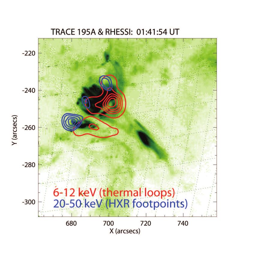
2      Loukas Vlahos, Sam Krucker and Peter Cargill

and the small-scale dissipation regions (≤ km) that evolve extremely rapidly
(seconds to minutes).
    The issues are well summarised in [143] where it is stated that “In fu-
ture, we hope for a closer link between the macroscopic MHD of the flare and
the microscopic plasma physics of particle acceleration. The global environ-
ment for particle acceleration is created by MHD, but there is a feedback, with
the MHD affected by the nature of the turbulent transport coefficients”. We
draw attention in particular to the word “feedback”: the fundamental ques-
tion which needs to be fully addressed is the following: can we disengage
the macroscopic MHD physics from the microscopic plasma physics
responsible for particle acceleration? Current observational and theoret-
ical developments suggest that for the case of explosive energy release in the
solar atmosphere, such a separation is not possible.
    The extraordinary efficiency of converting magnetic energy to energetic
particles during solar flares (almost 50% of the dissipated magnetic energy
will go into energetic particles, see Sect. 2), raises questions about the use of
macroscopic (ideal or resistive MHD) theories as the description of impulsive
energy release. The nonlinear coupling of large and small scales is extremely
difficult to handle just by the use of transport coefficients. This is a problem
which extends beyond solar physics and is one reason that our progress in
understanding solar flares has been relatively slow over the last hundred years
[34]. The overall goal of this paper is to show how alternative approaches
to the “flare problem” can begin to show how the integration of large-scale
magnetic field dynamics with particle acceleration processes is possible.
    In this review we present a radically different approach, used less in the
current literature, that connects the impulsive energy release in the corona
with the complexity imposed in active regions by the turbulent photospheric
driver [165]. The flare problem is thus posed differently, since it emerges nat-
urally from the evolution of a complex active region. The convection zone ac-
tively participates in the formation and evolution of large scale structures by
rearranging the position of the emerged magnetic field lines. At the same time
the emergence of new magnetic flux rearranges the existing magnetic topolo-
gies in complex ways. 3-D magnetic topologies are thus constantly forced away
from a potential state (if they were ever in one at all) due to slow (or abrupt)
changes in the convection zone. Within these stressed large-scale magnetic
topologies, localized short-lived magnetic discontinuities (current sheets) form
spontaneously, and dissipate the excess energy in the form of small or large
scale structures (nanoflares and flares/CMEs). We stress that the concept
of the sudden formation of a distribution of unstable discontinuities inside a
well organized large-scale topology is relatively new in the modeling of the
solar flare phenomenon (see for example [137, 128] for important steps in the
development of this approach).
    The scenario of spatially distributed self-similar current sheets with lo-
calized dissipation evolving intermittently in time is supported by observa-
tions which indicate that flares and intense particle acceleration are associ-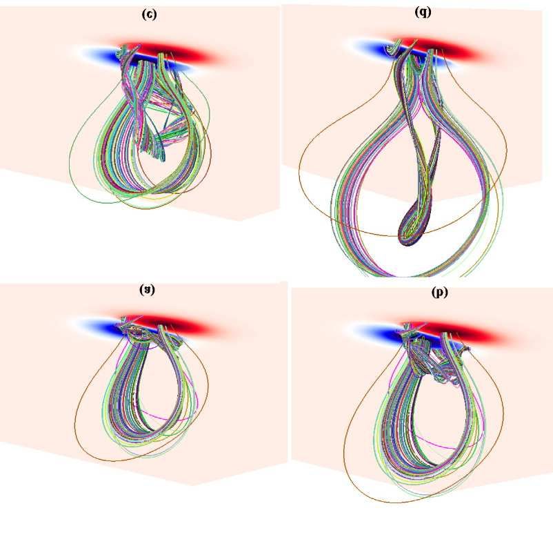
The Solar Flare: A Strongly Turbulent Particle Accelerator        3

ated with fragmented energy dissipation regions inside the global magnetic
topology [168, 25]. There is strong evidence that narrow-band milli-second
spike-emission in the radio range is directly associated with the primary en-
ergy release. Such emission is fragmented in space and time, as seen in radio-
spectrograms and in spatially resolved observations [173]. It can then be sug-
gested that the energy release process is also fragmented in space and time,
to at least the same degree as the radio spike-emission [24]. Also type III
burst radio-emission, caused by electron beams escaping from flaring regions,
appear in clusters, suggesting that fragmentation is a strong characteristic of
the flaring region [23].
    One approach which is able to capture the full extent of this interplay of
highly localized dissipation in a well-behaved large scale topology (‘sporadic
flaring’) is a special class of models [109, 110, 167, 115, 81, 82] which implement
the concept of Self-Organized Criticality (SOC), proposed initially by Bak et
al. [19]. The main idea is that active regions evolve smoothly until at some
point(s) inside the large scale structure magnetic discontinuities (of all sizes)
are formed and the currents associated with them reach a critical threshold.
This causes a fast rearrangement of the local magnetic topology and the release
of excess magnetic energy at the unstable point(s). This rearrangement may
in turn cause a lack of stability in the immediate neighborhood, and so on,
leading to the appearance of flares (avalanches) of all sizes that follow a well
defined statistical law which agrees remarkably well with the observed flare
statistics [38].
    Based on the current observational and theoretical evidence discussed in
this review, we suggest that our inability to describe properly the coupling be-
tween the MHD evolution and the kinetic plasma aspects of a driven flaring
region is the main reason behind our lack of understanding of the mecha-
nism(s) which causes flares and the acceleration of high energy particles. Let
us now define the ‘acceleration problem’ during explosive energy release in
the sun: We need to understand the mechanism(s) which transfer more than
50% of magnetic energy to large numbers (1039 particles in total) of ener-
getic electrons and ions, to energies in the highly relativistic regime (> 100
MeV for electrons and tens of GeVs for ions) on a short time scale (seconds
or minutes), with specific energy-spectra for the different isotopes and charge
states.
    In Section 2 we briefly describe the key observational constrains. In Section
3 we present a brief overview of the main theories for impulsive magnetic
energy release and in Section 4 we concentrate on the mechanisms on particle
acceleration inside a more realistic and complex magnetic topologies. Finally
in in Section 5 we discuss the ability of the proposed accelerators to explain
the main observational results and in Section 6 we report the main points
stressed in this review.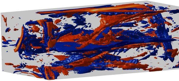
4                   Loukas Vlahos, Sam Krucker and Peter Cargill

2 Observational Constraints

2.1 X-rays observations: diagnostics of energetic electrons and
thermal plasmas

Energetic electrons produce X-ray emission by collisions (the radiation mecha-
nism responsible for the emission is non-thermal bremsstrahlung). The denser
the plasma, the more collisions, and the more X-rays are produced (see Fig.
1). Therefore, X-rays produced by non-thermal electrons are strongest from
the chromospheric footpoints of loops where the density increases rapidly.
Indeed as the energetic electrons move into the chromosphere, they eventu-
ally lose all their energy through collisions. This scenario is usually called the
“thick-target model” [30]. X-ray bremsstrahlung emission is in principle
also emitted in the corona but the lower density there (∼ 109 particles/cm3 )
is not big enough to stop energetic electrons or indeed to make them lose a
significant amount of their energy (“thin-target model”). The estimated mean
free path of an electron in the corona is > 105 km. In general present day in-
strumentation does not have a high enough signal to noise ratio to detect faint
thin-target bremsstrahlung emission from the corona next to much brighter
footpoints.

                              TRACE 195A: 29-Oct-2003 20:52:15.000 UT                               TRACE 171A: 15-Aug-2004 03:29:49.000 UT
                   -300
                                                                                            -220

                   -320
                                                                                            -240

                   -340
                                                                                            -260
                                                                              Y (arcsecs)
     Y (arcsecs)

                   -360
                                                                                            -280

                   -380
                                                                                            -300

                   -400
                                                                                            -320

                   -420
                               15-20 keV                                                    -340   PIXON 25-100 keV (grid 1-6; 30,50,...%)
                               50-100 keV                                                          PIXON 6-12 keV (grid 1-6; 3,5,10,30,...%)
                   -440
                          0      20    40    60      80    100   120    140                         600   620   640       660     680   700   720
                                             X (arcsecs)                                                              X (arcsecs)

Fig. 1. Two examples of X-ray imaging in solar flares: (left) a large flare near disk
center, (right) a small compact flare. Thermal emission in X-rays is shown by red
contours, while non-thermal emission is shown as blue. The green images show EUV
emission observed by TRACE with dark colors corresponding to enhanced intensity.

     Thermal plasmas with temperatures above 1 MK also radiate in X-rays
by collisions (thermal bremsstrahlung). Thermal X-ray spectra have a steeply
falling continuum component plus some line emissions. In solar flares, thermal
emission generally dominates the X-ray spectrum below 10-30 keV. At higher
energies, the flare spectra are generally flatter, having power laws with indices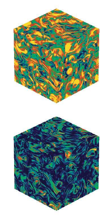
The Solar Flare: A Strongly Turbulent Particle Accelerator                                         5

between 3-5, sometimes with breaks (see Fig. 2). This is the non-thermal
bremsstrahlung component produced by energetic electrons.

                                                                                                               flare peak: 20-Jan-2005 06:45:10.994 UT
                                                   104                                             320

         X-ray spectrum [photons s-1 cm-2 keV-1]
                                                                                                   300

                                                        2
                                                   10                                              280

                                                                                     Y (arcsecs)
                                                                                                   260

                                                        0                                          240
                                                   10

                                                                                                   220

                                                                                                   200                       12-15 keV (thermal)
                                                   10-2
                                                                                                                             250-500 keV (non-thermal)
                                                                                                   180                       TRACE 1600A (image)
                                                                                                         780     800   820     840     860   880   900   920
                                                                10             100                                             X (arcsecs)
                                                                     energy [keV]

Fig. 2. Spectroscopy and imaging in X-rays: (left) a spatially integrated X-ray
spectrum with a thermal fit in red and a broken power law fit (non-thermal emission)
in blue. The data is shown in black and the instrumental background emission is
shown in grey. (right) X-ray imaging with thermal emission in red and non-thermal
in blue.

2.2 Energy estimates

Spectral X-ray observations provide quantitative estimates of the energy con-
tent. The non-thermal energy (i.e. the energy in the accelerated energetic
electrons) can be estimated by inverting the photon spectrum to get the elec-
tron spectrum. The total energy is then derived by integrating the electron
spectrum above a cutoff energy. The largest uncertainties in this derivation are
due to the not-well-known cutoff energy. Often only an upper limit is known,
giving lower limits to the non-thermal energy. Current estimates suggest that
almost 50% of the total flare energy is deposited in energetic particles [56, 57].
    Thermal flare energies are derived by fitting the thermal part of the X-ray
spectra with a single temperature model, thus providing estimates of tem-
perature and emission measure EM ∼ n2 V . Here V is an estimate of the
volume occupied by the thermal plasma, usually obtained from images. From
the emission measure and the volume, the number of heated electrons can be
determined, each of which contains 1.5kT J. Assuming     pthe same number of
ions are heated, the total thermal energy becomes 3kT EM/V . This energy
estimate is equal to the total energy needed to obtain the observed heated
flare plasma and does not account for radiative and conductive losses. The
derived energies are therefore only lower limits.
    In solar flares, the thermal and non-thermal energy estimates are generally
correlated and are often the same order of magnitude. This is consistent with
6      Loukas Vlahos, Sam Krucker and Peter Cargill

the picture that flare energy release first accelerates electrons which later lose
their energy by collisions, heating chromospheric plasma (see [149] for recent
results and references therein).

2.3 Temporal correlation

Neupert effect

If the flare-accelerated energetic electrons indeed heat the flare plasma, the
X-ray time profile of the thermal and non-thermal emission should reflect
this: the non-thermal X-ray time profile should be a rough measure of how
much energy is released in non-thermal electrons, and this is then the energy
available for heating. So the larger the non-thermal X-ray flux, the more
heating is expected. The time history of the integrated non-thermal X-ray
flux roughly corresponds to the time profile of the thermal X-ray emission
(this is called Neupert effect: see [162] for recent results).

Fig. 3. Top: The spectral index (thin line) and flux (thick line) obtained from the
uncalibrated total count rates flux in the energy bands 26-35 keV and 35-44 keV
and their ratio. Bottom: the spectral index γ (thin line) and non-thermal flux F35
at 35 keV in photons s−1 cm−2 keV−1 (thick line) for the event of 9 November 2002,
obtained by spectral fitting [70].
The Solar Flare: A Strongly Turbulent Particle Accelerator       7

Spectral evolution: soft-hard-soft

A very strong temporal correlation is observed between the non-thermal X-
ray flux and the power law index of the photon spectrum: for each individual
peak in the time series, the spectral shape hardens (flatter spectrum) until
the peak and then softens (steeper spectrum) again during the decay (Fig.
3). This is referred to as the soft-hard-soft effect [70, 71] and seems to be a
specific characteristic of the acceleration process. It is not understood. In some
flares, the spectral behavior is different showing a gradual hardening during
rise, peak, and decay for each individual burst. These events tend to be large
and have a very good correlation with flares related to solar energetic particle
(SEP) events [86]. Their behavior is also not understood. Note that spectral
hardening can occur if electrons are trapped and low energy particles are lost
first.

2.4 Location of energy release

Coronal Hard X-ray (HXR) sources

Coronal X-ray emission is most often from hot thermal loops as described
above. However, for some events an additional X-ray source is observed orig-
inating above the thermal X-ray loops [112], called an ‘above the loop top
source’ (ALT). First observed by Yohkoh, and only seen in a few flares (see
Fig. 4), these sources are generally fainter with a softer spectrum than X-ray
footpoints sources. There is no agreed interpretation of them at this time.
If the footpoints and the ALT source are all produced by the same popula-
tion of energetic electrons, the location of the ALT source indicates that the
acceleration does not happen inside the flare loop. Therefore, it is generally
speculated that the acceleration occurs above that loop. The relatively small
number of flares with ALT sources might be because of the limited dynamic
range of the observations alluded to earlier.
    Several events do not follow this simple picture and the source is more
complicated (see Fig. 5). RHESSI observations show several clear examples of
ALT sources: the time evolution of these sources shows fast variations with
several peaks of tens of second duration. The observed spectra are rather soft
with power law indices around 5 and are better represented by non-thermal
(power law) spectra than by thermal fits, although multi-thermal fits with
temperatures up to 100 MK can represent the data almost as well. The fast
time variations are very difficult to explain for a thermal interpretation (i.e.
repeated heating to 100 MK and cooling on the same time scale). However,
there are also difficulties with the non-thermal interpretation: the HXR pro-
ducing electrons should significantly heat the ALT, but the hot thermal loops
are observed below it.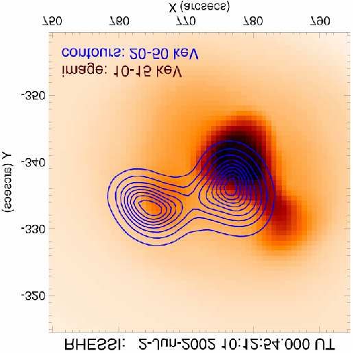
8       Loukas Vlahos, Sam Krucker and Peter Cargill

Fig. 4. Hard X-ray and soft X-ray images of the 13 January 1992 flare. The leftmost
panel shows a soft X-ray image taken with the Yohkoh/SXT Be filter at 17:28:07 UT.
From left to right, the remaining three panels show images contours at 14-23, 23-33,
and 33-53 keV, respectively, taken from 17:27:35 - 17:28:15 UT by Yohkoh/HXT,
overlaid on the same soft X-ray image. The contour levels are 6.25, 12.5, 25.0 and
50% of the peak value. The field of view is 59′′ × 79′′ for all panels.

Fig. 5. X-ray imaging of a complex flare: the image (red) shows the thermal emission
as seen by RHESSI at 10-15 keV, and the non-thermal emission is again given by
blue contours

Time of flight

Further support for acceleration above the thermal flare loops is provided by
timing studies of HXR footpoints at different energies. If energetic electrons at
different energies are accelerated almost simultaneously at the same location,
time of flight effects from the acceleration site to the HXR footpoints should
be observed. This is indeed observed and it allows one to estimate the path
length from the acceleration site to the HXR footpoints. The derived path
lengths are generally longer than half the length of the flare loops connecting
the HXR footpoints [16]. Although the error bars are large, this again suggests
that the acceleration occurred above the flare loops.
The Solar Flare: A Strongly Turbulent Particle Accelerator      9

Temperature structure

Recent RHESSI observations also show support for particle acceleration above
the main flare loop [157]. Evidence was found for a temperature gradient with
decreasing temperatures from the possible coronal acceleration site towards
lower and higher altitudes [156]. The hottest flare loops are expected to be the
newly reconnected loops at largest altitude. Previously heated flare loops are
at lower altitude and have already partly cooled down. For energetic electrons
released upwards, the opposite is expected with the hottest emission at lowest
altitude, as observed. Another explanation could be that there is direct heating
at the particle acceleration site (as a by-product of the main acceleration
process) that would produce a similar temperature profile.

2.5 Footpoint motions

Standard magnetic reconnection models predict increasing separation of the
footpoints during the flare [143] as longer and larger loops are produced. If the
reconnection process results in accelerated electrons [131], the HXR footpoints
should show this motion. The motion is only apparent; it is due to the HXR
emission shifting to footpoints of neighboring newly reconnected field lines.
Hence, the speed of footpoint separation reflects the rate of magnetic recon-
nection and should be roughly proportional to the total HXR emission from
the footpoints. Sakao, Kosugi, & Masuda [150] analyzed footpoint motions
in 14 flares observed by Yohkoh HXT, but did not find a clear correlation
between the footpoint separation speed and the HXR flux. Recently, how-
ever, source motion seen in Hα was studied by Qiu et al. [146]. They found
some correlation with HXR flux during the main peak, but not before or after.

    RHESSI results [59, 91, 92, 71] show systematic but more complex foot-
point motions than a simple flare model would predict. Krucker, Hurford, &
Lin [93] analyzed HXR footpoint motions in the July 23, 2002 flare (GOES
X4.8-class). Above 30 keV, at least 3 HXR sources are observed during the
impulsive phase that can be identified with footpoints of coronal magnetic
loops that form an arcade. On the northern ribbon of this arcade, a source
is seen that moves systematically along the ribbon for more than 10 minutes.
On the other ribbon, at least two sources are seen that do not seem to move
systematically for longer than half a minute, with different sources dominat-
ing at different times. The northern source motions are fast during times of
strong HXR flux, but almost absent during periods with low HXR emission.
This is consistent with magnetic reconnection if a higher rate of reconnection
(resulting in a higher footpoint speed) produces more energetic electrons per
unit time and therefore more HXR emission. The absence of footpoint motion
in one ribbon is inconsistent with simple reconnection models, but can be
explained if the magnetic configuration is more complex. Also the motion of
the northern footpoint is rather along the ribbon, contrary the perpendicular
10      Loukas Vlahos, Sam Krucker and Peter Cargill

motions predicted by simple reconnection models. In some events the motion
during the whole flare is clearly along the ribbons [71].

2.6 Gamma Rays (emission above > 300 keV)
Electron bremsstrahlung
The non-thermal electron bremsstrahlung component can extend up to and
above 10 MeV. This component is produced in the same way as the emission
seen above 20 keV, but from electrons with higher energies. Generally the
spectrum shows a hardening (flatter spectrum) above 0.5-1 MeV. Because
the spectrum decreases steeply with energy, electron bremsstrahlung in the
gamma-ray range is only observed for very large flares. Rarely, however, is it
the dominant emission in the gamma-ray range. For most gamma ray flares,
emission produced by energetic ions is present as well.

Fig. 6. Composite X-ray/gamma-ray spectrum from 1 keV to 100 MeV for a large
flare. At energies up to 10-30 keV, emission from hot (107 )and ’superhot’ (3 × 10⁷ )
thermal flare plasmas (the two curves at the left) dominate. Bremsstrahlung emission
from energetic electrons produces the X-ray/gamma-ray continuum (straight lines)
up to tens of MeV. Broad and narrow gamma-ray lines from nuclear interactions
of energetic ions sometimes dominate the spectrum between 1 to 7 MeV. Above a
few tens of MeV the photons produced by the decay of pions (curve at the right)
dominates. RHESSI observations cover almost four orders of magnitude in energy
(3 keV to 17 MeV) [104].
The Solar Flare: A Strongly Turbulent Particle Accelerator    11

De-excitation lines
Flare-accelerated ions (protons, alphas, heavier ions) are responsible for the
production of gamma ray emission when they collide with ambient ions and
produce excited nuclei that emit nuclear de-excitation lines. Again, the emis-
sion process depends on the density of the ambient plasma and therefore the
emission is expected from dense regions (i.e. the chromosphere). Since the
de-excitation is happening almost instantaneously after the collision, these
gamma ray lines are also referred to as prompt lines. Depending on the ratio
of the mass of the accelerated ion to the target ion, the line emission can be
narrow or broad. Narrow lines are produced when a flare-accelerated proton
or alpha particle hit a heavy ambient ion. The width of the emitted line is
then produced by the recoil of the heavy ambient ion, and a narrow line is
produced. On the other hand, if a heavy flare-accelerated ion hits an am-
bient proton or alpha particle, the emitted radiation is Doppler-shifted and
therefore broad.
    RHESSI provides for the first time spectrally resolved observations of nar-
row de-excitation lines. Statistics are generally limiting the observations, but
the narrow lines can still be fitted and the red shift of the lines can be mea-
sured. Heavier nuclei are expect to recoil less and therefore show less redshift
[155].

Neutron Capture Line
The most prominent line emission in the gamma ray spectrum is the neutron
capture line at 2.223 MeV. This line is produced by the capture of thermalized
neutrons that were produced by nuclear reactions after flare-accelerated ions
hit ambient ions (the dominant neutron production at high energies comes
from the breakup of He). The thermalized neutrons are captured by ambient
protons and a deuterium and a photon at 2.223 MeV are produced. Since the
neutrons are thermalized (i.e. have a low velocity) the 2.223 MeV line is very
narrow. Since initially the neutrons have to first thermalize before they can
be captured, the time profile of the 2.223 MeV line is delayed relative to the
prompt lines.

Energy estimates
The different gamma-ray lines can be used to get information about the flare
accelerated ion spectrum. Estimates of the total energy in non-thermal ions
can again be derived by integrating over the ion spectrum. The lower energy
cutoff, however, is even more uncertain than for the electron spectrum.

Comparing electron and ions acceleration
Comparing the fluence of > 300 keV emission with the fluence of the 2.2 MeV
line, the electron and ion acceleration in flares can be compared. A rough cor-
12 Loukas Vlahos, Sam Krucker and Peter Cargill
Fig. 7. RHESSI gamma ray spectrum of the July 23, 2002 flare.
relation is observed indicating that at least in very large flares (gamma-ray
emission from small flares are not detectable with present day instrumenta-
tion), both electrons and ions are always accelerated.
Gamma ray imaging
RHESSI provides for the first time spatial information of gamma ray emission,
the only direct indication of the spatial properties of accelerated ions near the
Sun. The most powerful tool for gamma ray imaging is the 2.223 MeV neutron
capture line, because of good statistics and a narrow line width which limits
the non-solar background to a minimum compared to broad lines. However,
the spatial resolution of 35” is much poorer than the 2” resolution in the hard
X-ray range
For the event with best statistics (October 28, 2003 [79]), the 2.223 MeV
source structure shows two footpoints similar to the HXR source structure
but clearly displaced by ∼15” (see Fig. 8). This indicates that electrons and
ions are accelerated in similar-sized magnetic structures. The displacement
could be explained by different accelerator sites for electrons and ions, or by
different transport effects from a possibly common acceleration site to the
location where the electrons and ions lose their energy by collisions.The Solar Flare: A Strongly Turbulent Particle Accelerator 13
TRACE & RHESSI: 28-Oct-2003 11:06:46.000 UT
-250
-300
-350
Y (arcsecs)
-400
-450
2223 keV
100-200 keV
-200 -150 -100 -50 0
X (arcsecs)
Fig. 8. Imaging of the 2.223 MeV neutron-capture line and the HXR electron
bremsstrahlung of the flare on October 28, 2003. The red or gray circles show the
locations of the event-averaged centroid positions of the 2.223 MeV emission with
1σ uncertainties; the blue or black lines are the 30, 50, and 90% contours of the
100 - 200 keV electron bremsstrahlung sources at around 11:06:46UT. The under-
lying EUV image is from TRACE at 195Å with offset corrections applied. The
gamma-ray and HXR sources are all located on the EUV flare ribbons seen with
TRACE.
2.7 Energetic particles escaping from the sun
Flare accelerated electrons escaping the Sun
X-rays are remote sensing diagnostics of energetic electrons that lose their
energy by collisions. Upward moving energetic electrons that have access to
field lines extending into interplanetary space (often referred to as “open field
lines”) only suffer a few collisions (the density is decreasing rapidly) and can
therefore escape from the Sun and be observed in-situ near the Earth with
particle detectors. These events show fast rise times with slow decays and are
called ‘impulsive electrons events’ when observed near Earth [105]. They are
seen with energies from above 1 keV up to the highly relativistic regime. Quite
often the first electrons to arrive are observed to travel without suffering any
collisions (ballistic transport) and they are therefore referred to as “scatter-
free” events. The ballistic transport means that high energy electrons arrive
earlier than lower energy ones, indicating that electrons at all energies left
the Sun around the same time. The observed dispersion in the onset times of14 Loukas Vlahos, Sam Krucker and Peter Cargill
the different energy channels can therefore be used to approximate when the
energetic electrons left the Sun. In some case (about one third of all events) a
clear temporal correlation exists with the occurrence of HXR emission during
solar flares and the release of energetic electrons into interplanetary space
(Fig. 9a).
This indicates that possibly the same acceleration mechanism produces
the energetic electrons that create HXR emission in the chromosphere and
those energetic electrons that escape into interplanetary space. This picture
can be further corroborated by comparing the HXR spectrum with the in situ
electron spectrum. If the chromospheric X-ray spectrum is flat (hard), the
electron spectrum observed near Earth ia also flat (Fig. 9b).
10-5
frequency [MHz]
1.6 keV 12
GOES flux [Watt m-2]
10
10-6 8
6
3.1 keV 4
10-7 2
frequency [Hz]
10-8 105
150
counts s-1
100 104
50
electron flux [s-1 cm-2 ster-1 eV-1]
27 keV
40 keV
0 25-80 keV 10-2
66 keV
12
frequency [MHz]
10 10-3 108 keV
8
181 keV
6
510 keV
4 10-4 310 keV
2
2110 2115 2120 2130 2200
Fig. 9. Impulsive electron event observed on October 19, 2002: (left) From top
to bottom, GOES soft X-ray light curves, RHESSI 25-80 keV light curve, and
WIND/WAVES radio spectrogram in the 1 to 14 MHz range are shown [29]. (right)
An expanded view of the WIND/WAVES data including low frequency observations
is presented in the top two panels, while the bottom panel shows in-situ observed
energetic electrons from 30 to 500 keV detected by WIND/3DP. This event (like
all events selected in this survey) shows a close temporal correlation between non-
thermal HXR emission, radio type III emission in interplanetary space, and in-situ
observed electrons.
For particles to escape into interplanetary space, they must have access
to open field lines. How that happens is not well understood. In the “classic”
flare scenario (e.g. [153]) no open field lines are shown. For flares with aThe Solar Flare: A Strongly Turbulent Particle Accelerator 15
good temporal and spectral correlation with electron events observed in situ,
the flare geometry indeed looks different. These events show hot flare loops
with HXR footpoints, plus an additional HXR source separated from the loop
by 15” with only little heating. This source structure can be explained by
a simple magnetic reconnection model with newly emerging flux tubes that
reconnect with previously open field lines, so-called interchange reconnection.
The previously open field lines form the flare loops, while the newly opened
field lines show less heating since material can be easily lost because the field
is open. Upwards moving energetic electrons escape along the newly opened
field line (see Fig. 10).
T R A C E 1 9 5 A & R H E S S I: 0 1 :3 9 :2 2 .0 U T
-2 2 0
HXRs
-2 4 0
Y (a rc s e c s )
HXRs
-2 6 0
escaping electrons
acceleration
region
HXRs EUV jet
-2 8 0
6 -1 2 k e V
-3 0 0 2 0 -5 0 k e V
660 680 700 720 740
X (a rc s e c s )
Fig. 10. EUV and X-ray sources of a flare that released energetic electrons into
interplanetary space that were later observed near the Earth.
Left figure: RHESSI contours at 6 - 12 keV (red or dark gray: thermal emission)
and 20 - 50 keV (blue or black: non-thermal emission) overlaid on a TRACE
195Å EUV image (dark region corresponds to enhanced emission). Located at
around [700, -245] arcsec, the X-ray emission outlines a loop with two presumably
nonthermal footpoints. The strongest footpoint source however, is slightly to the
southeast [683, -257] and shows a surprisingly lower intensity thermal source.
Right figure: Suggested magnetic field configuration showing magnetic reconnection
between open and closed field lines inside the red or dark gray box marked as the
“acceleration region” where downward moving electrons produce the HXR sources
and upward moving electrons escape into interplanetary space.16 Loukas Vlahos, Sam Krucker and Peter Cargill
Flare accelerated ions escaping from the Sun
Temporal and spectral comparisons can also be made for ions escaping from
the Sun in a similar way to escaping electrons. However, this is much more
difficult to do because of the poorer count statistics in the gamma ray range.
The timing of escaping ions is sometimes delayed relative to the flare emis-
sion, often significantly (1hour) [94]. Generally it is thought that the shocks
of Coronal Mass Ejections are mainly responsible for the energetic ions seen
near to the Earth. If this is indeed the case, then a spectral comparison be-
tween in-situ observed ion spectra and gamma ray line observations should
give no correlation. Surprisingly, in the two gamma-ray line flares observed
by RHESSI that are magnetically well-connected (2 Nov 2003 and 20 Jan
2005), the spectrum of the energetic protons producing the gamma-ray lines
was found to be essentially the same as that of the SEP protons observed at
1 AU. These two events had quite different spectral slopes, so this agreement
is unlikely to be a coincidence. It suggests that the gamma-ray producing
and in-situ energetic protons may have the same source (at least in these
two events), contrary to the standard two-class paradigm (i.e. flare acceler-
ated and CME accelerated ions). These results illustrate the present lack of
physical understanding regarding the SEP acceleration process(es).
2.8 Statistical properties of flares
Flares are not just simple explosions in the solar atmosphere. Even a sin-
gle “flare” shows many individual peaks during its evolution [70, 71]. When
observing an active region or the whole Sun for a certain period of time, a
number of flares with different total energy E (or peak energy Ep ) will be
recorded. If we define as F (E)dE the fraction of flares which released energy
between E and E +dE, then a very striking statistical feature of energy release
in active regions emerges [38]. The frequency distribution F (E) reconstructed
from UV, EUV and X-ray observations has a simple form (see Fig. 11)
F (E) = F0 E −a (1)
which holds for eight orders of magnitude in E. Similar laws are obtained
for the peak energy and the flare duration. The value of the exponent is
not constant and may range from 1.6 − 2.0, depending of the data set used.
Current instruments are not able to observe nano-flares (energies below 1024
ergs) and the lower part of the distribution, which plays a crucial role in
coronal heating, is uncertain. A key point for our discussion here is that the
energy release of the active region is self similar. This particular feature of
the observed characteristics of flares has created many heated discussions and
remain an open and difficult theoretical problem which will be discussed in
the next section.The Solar Flare: A Strongly Turbulent Particle Accelerator 17
Fig. 11. The frequency distribution of total flare energy, peak flux and duration
[38].
2.9 Summary of observational constrains and discussion
We now pull together the above results, and address their implications for
understanding flare particle acceleration. Of particular importance are the
implications arising from the thick target model:
1. The thick target model for HXR and its theoretical implica-
tions: The theoretical basis of the thick target model, as originally pre-
sented [30] and re-iterated recently [31], is based on the assumption that
the accelerator is located in the corona and the HXR source in the up-
per chromosphere. Thus the acceleration region is collision-free and the
radiation source is collision-dominated and electrons travel the distance
between acceleration region and radiation region ballistically [16]. A large
HXR burst flux suggests that the required electron flow rate is ≥ 103718 Loukas Vlahos, Sam Krucker and Peter Cargill
electrons/sec with electron energies above 20 keV. This amounts to a
total of 1039 electrons for a burst lasting several minutes. This result,
known as the number problem, implies that all the particles inside a
very large coronal volume (∼ 1030 cm3 , almost the entire corona above an
active region) are accelerated within a few minutes and stream towards
the chromosphere. Assuming that the acceleration is inside a large-scale
current sheet (see Fig. 12 and later discussion) with typical dimensions
1010 cm × 1010 cm × 105 cm, this monolithic current sheet must accelerate
all the particles entering it (the inflow velocity needs to be a fraction of
the local Alfven speed) and remain stable for tens of minutes. We return
to these points at the end of the Section.
2. Energetics: Assuming that ∼ 1039 electrons are accelerated with a mean
energy of 50 keV, the energy they carry is ∼ 1031 ergs. Since the accel-
erated particle fill a volume ∼ 1030 cm3 and if the mean magnetic field
available for dissipation in the corona is 30G, the available magnetic en-
ergy is ∼ 5 × 1031 ergs so a significant fraction of the magnetic energy in
this acceleration volume will go to the energetic electrons
3. Spectral index and low energy cut-off: The energetic particles form
a thermal distribution up to a critical energy Ec ∼ 1−30 keV and a power
law distribution above this energy. The spectral index (δ) varies both in
the course of the burst and from event to event but remains within the
range 2-6. The presence of multiple breaks at different energies is also
observed frequently.
4. The temporal evolution of the power law index: The power law
index varies during the impulsive phase of the flare, following a specific
evolution: soft-hard-soft.
5. Acceleration time: The accelerator should start on sub-second timescales
and remain on for tenths of minutes for the electrons. Ions are also accel-
erated in secs and the accelerator remains active (sometimes) for hours.
6. Maximum energy: The maximum energy achieved is close to hundreds
of MeV for the electrons and several GeV for the ions.
7. Flare statistics: The flares released in a specific active region are not
random. They follow a specific statistical law in energy, peak intensity
and duration.
8. Footpoint motion: According to the “standard model” (see below) re-
connection causes the footpoints to move smoothly away from each other
or along the filament. Some observations seem to support this prediction
but others not, so the motion of the footpoints is still an open question.
9. The coronal sources: Coronal sources at 20 - 30 keV are hard to confine
collisionally, therefore the fact that they persist as isolated blobs in space,
their characteristic spectral evolution, and their movement, remain open
theoretical challenges.
10. The close time and spectral evolution of the two footpoints: When
the two footpoints appear (usually in energies above 30 keV), they seem
to correlate in temporal and spectral evolution leaving the impressionThe Solar Flare: A Strongly Turbulent Particle Accelerator 19
that the accelerated particles moving in them are coming from the same
acceleration source.
11. Interplanetary energetic particles: There is a close correlation of the
HXR index with the properties of energetic particles detected in the inter-
planetary medium. This appears to need more complex magnetic topolo-
gies that currently discussed at the Sun.
12. High energy Ions: There is an observed shift in the location of ion and
electron footpoints. Sometimes, contrary to the electrons, the energetic
ions show a single foot point. The acceleration of ions and electrons in
different length loops and the loop anisotropy with the low sensitivity are
two explanations offered so far. There is an apparent correlation between
electron acceleration above 300 keV and ion acceleration. The correlation
of relativistic electron and ions, and the fact that the spectrum of electrons
above 300 keV remains a power law with harder spectrum, recalls an older
suggestion for two-stage acceleration, where shock acceleration may play
an active role in the second stage in some large flares.
From the above summary, several important points arise, many concerning
the efficiency requirements of the thick target model. It is especially interesting
to discuss this in the context of what is sometimes referred to the “standard
flare mode” as shown in Fig. 12. This orignated in old models for long-decay
flares [33, 90], and has been proposed as a generic scenario for coronal flaring.
In particular, the model invokes a monolithic current sheet, which, one must
assume, is where the particle acceleration takes place. In fact, as we will show
in the next section, it is rather difficult to achieve efficient acceleration in
simple magnetic topologies.
There are major electrodynamic constraints arising in the thick target
model. The large flux of energetic electrons (F37 ∼ 1037 electrons/sec) flowing
through a relatively small area (the observed footpoints are relatively compact
with characteristic area A17 ∼ 1017 cm2 ) suggests that the beam density of
the energetic electrons (mean velocity 1010 cm/sec), can be as high as nb ∼
1010 electrons/cm3. Assuming that the ambient density at the HXR source is
comparable or one order of magnitudes higher (n0 ∼ 1011 particles/cm3 ), a
neutralising return current is required with a characteristic velocity of vr ∼
109 cm/sec. The return current replenishes the already-accelerated particles
in the acceleration volume with hot plasma if the acceleration region and
radiation region are magnetically connected. The observed hot thermal loops
and the Neupent effect can be the observational tests for the reaction of the
chromosphere to this intense electron beam injected from the corona. This
vital point is not incorporated in current flare models, and the problem of
particle replenishment remains an open issue.
We also note that the scenario adopted for the thick target model for HXR
and the “standard flare model” leave number of open questions: (1) How is a
correlation between HXR and Type III bursts established? (2) The density of
the beams driving the normal type III burst (nb (III) ∼ 106 electrons/cm3 ) are20 Loukas Vlahos, Sam Krucker and Peter Cargill
Fig. 12. This cartoon, suggested several years ago remains the favorite model and
was elevated recently to the “standard flare cartoon”. It has been in the literature
for many years, it was revised to incorporate more recent observation and it has
been born out in simple 2-D simulations. [153]
several orders of magnitude less than the beam density needed to power the
3
HXR through the thick target (nb (HXR) ∼ 1010 electron/cm ). What caused
this large imbalance? (3) The chromospheric evaporation will refill the loops
with plasma in seconds, but if the acceleration and the energy release is above
the loop(s) and the collapsing process for the formation of the loops has been
completed, how is the plasma inside the loop is re-accelerated?
We conclude that the standard 2-D flare cartoon shown in Fig. 12 and/or
2-D simulations based on the cartoon, are not able to handle the relevant
physics question. Eruption in 3-D magnetic topologies is still an active research
project and the simple magnetic topology presented in Fig. 12 can mainly be
used to represent an idea of how the overall magnetic structure may respond
when energy is released during a CME/flare. We will return on this issue in
the next section.
The above constraints for the energy release and the subsequent acceler-
ation of high energy particles during large flares are hard to reconcile with
reconnection theory as hosted in a simple magnetic topology and associated
with a particular acceleration mechanism (DC electric fields, shocks or MHD
waves). However, this discussion should not be construed as an objection to
the role of reconnecting current sheets in flare acceleration and particle trap-
ping per se. It is a characteristic of the magnetohydrodynamic equations thatThe Solar Flare: A Strongly Turbulent Particle Accelerator 21
they are “self-similar” over a wide range of scales: in other words the accelera-
tion and heating is not just restricted to the large monolithic sheet, but occurs
at current sheets of all sizes. In the following sections we discuss in more detail
recent developments in the formation of the magnetic environment for particle
acceleration, and try to relate these topologies with mechanisms for particle
acceleration.
3 Models for impulsive energy release
3.1 3-D extrapolation of magnetic field lines and the formation of
unstable current sheets
The energy needed to power solar flares is provided by photospheric and sub-
photospheric motions and is stored in non-potential coronal magnetic fields.
Since the magnetic Reynolds number is very large in the solar corona, MHD
theory states that magnetic energy can only be released in localized regions
where the magnetic field forms small scales and steep gradients, i.e. in thin
current sheets (TCS).
Numerous articles (see recent reviews [46, 107]) are devoted to the anal-
ysis of magnetic topologies which can host TCSs. The main trend of current
research in this area is to find ways to realistically reconstruct the 3-D mag-
netic field topology in the corona based on the available magnetograms and
large-scale plasma motions at the photosphere. One must then search for the
location of special magnetic topologies, i.e. separatrix surfaces (places were
field lines form null points [99] and bald patches [158]), and more gener-
ally Quasi-Separatrix Layers (QSL) which are regions with drastic changes of
the field line linkage [46]. A variety of specific 3-D magnetic configurations
(fans, skeletons etc) have been analyzed, and their ability to host fast dif-
fusion of the magnetic field lines has also been investigated [143]. The main
analytical and computational approaches through which these structures are
analysed are based on prescribed and simple magnetic structures at the photo-
sphere, e.g. a quadrupole [17] (see Fig. 13). A realistic magnetic field generates
many “poles and sources” [107] and naturally has a relatively large number
of TCSs. We feel that this detailed representation of topological forms of
the TCSs is mathematically appealing for relative simple magnetic topologies
(dipoles, quadrupoles, symmetric magnetic arcades [17]). When such topo-
logical simplicity at the photosphere is broken, for example due to large-scale
sub-Alfv́enic photospheric motions or the emergence of new magnetic flux that
disturbs the corona, such tools may be less useful. All these constraints re-
strict our ability to reconstruct fully the dynamically evolving magnetic field
of an active region (and it is not clear that such a reconstruction will ever be
possible).
Many of the widely used magnetograms measure only the line of sight
component of the magnetic field. The component of the magnetic field vertical22 Loukas Vlahos, Sam Krucker and Peter Cargill
Fig. 13. Projected view of the two stressed magnetic field configurations used as
initial conditions for the search of QSL’s [17] .
to the surface matches the measured magnetic field only at the center of
the disk and becomes increasingly questionable as the limb is approached.
Extrapolating the measured magnetic field is relatively simple if we assume
that the magnetic field is a force-free equilibrium:
∇ × B = α(x)B (2)
where the function α(x) is arbitrary except for the requirement B ·∇α(x) = 0,
in order to preserve ∇ · B = 0. Eq. (2) is non-linear since both α(x) and
B(x) are unknown. We can simplify the analysis of Eq. 2 when α=constant.
The solution is easier still when α = 0, which is equivalent to assuming the
coronal fields contain no currents (potential field), hence no free energy, and
thus uninteresting.
A variety of techniques have been developed for the reconstruction of the
magnetic field lines above the photosphere and the search for TCSs [107, 113].
It is beyond the scope of this article to discuss these techniques in detail. For
instructive purposes, we use the simplest method available, a linear force
free extrapolation, and search for “sharp” magnetic discontinuities in the
extrapolated magnetic fields. Vlahos and Georgoulis [171] use an observed
active-region vector magnetogram and then: (i) resolve the intrinsic azimuthal
ambiguity of 180o [65], and (ii) find the best-fit value αAR of the force-free
parameter for the entire active region, by minimizing the difference between
the extrapolated and the ambiguity-resolved observed horizontal field (the
“minimum residual” method of [102]). They perform a linear force-free ex-
trapolation [6] to determine the three-dimensional magnetic field in the active
region. Although it is known that magnetic fields at the photosphere are not
force-free [67], they argue that a linear force-free approximation is suitable for
the statistical purposes of their study.
Two different selection criteria were used in order to identify potentially
unstable locations (identified as the afore-mentioned TCSs) [171]. These are
(i) the Parker angle, and (ii) the total magnetic field gradient. The angu-
lar difference ∆ψ between two adjacent magnetic field vectors, B1 and B2 , isThe Solar Flare: A Strongly Turbulent Particle Accelerator 23
given by ∆ψ = cos−1 [B1 ·B2 /(B1 B2 )]. Assuming a cubic grid, they estimated
six different angles at any given location, one for each closest neighbors. The
location is considered potentially unstable if at least one ∆ψi > ∆ψc , where
i ≡ {1, 6} and ∆ψc = 14o . The critical value ∆ψc is the Parker angle which, if
exceeded locally, favors tangential discontinuity formation and the triggering
of fast reconnection [136, 137]. In addition, the total magnetic field gradient
between two adjacent locations with magnetic field strengths B1 and B2 is
given by |B1 − B2 |/B1 . Six different gradients were calculated at any given
location. If at least one Gi > Gc , where i ≡ {1, 6} and Gc = 0.2 (an arbi-
trary choice), then the location is considered potentially unstable. When a
TCS obeys one of the criteria listed above, it will be transformed to an Un-
stable Current Sheet (UCS). A steep gradient of the magnetic field strength,
or a large shear, favors magnetic energy release in three dimensions in the ab-
sence of null points [144]. [Note that these thin elongated current sheets have
been given different names by different authors: e.g. in [17] they are called
Hyberbolic Flux Tubes.]
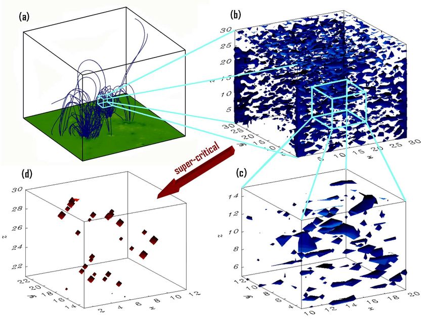
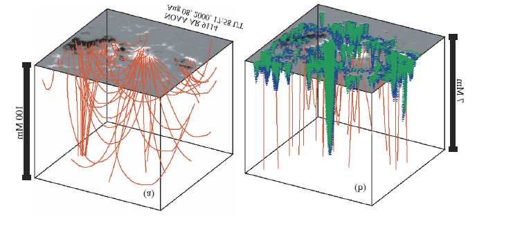
Fig. 14. (a) Linear force free field extrapolation in NOAA AR 9114, (b) Lower part
of the AR atmosphere. Shown are the magnetic field lines (red) with the identified
discontinuities for critical angle 10◦ [171].
Potentially unstable volumes are formed by the merging of adjacent se-
lected locations of dissipation. These volumes are given by V = N λ2 δh, where
N is the number of adjacent locations, λ is the pixel size of the magnetogram
and δh is the height step of the force-free extrapolation. The free magnetic
energy E in any volume V is given by
N
λ2 δh X
E= (Bff l − Bp l )2 (3)
2µ0
l=1
where Bff l and Bp l are the linear force-free and the potential fields at location
l respectively. The assumption used is that any deviation from a potential24 Loukas Vlahos, Sam Krucker and Peter Cargill
configuration implies a non-zero free magnetic energy which is likely to be
released if certain conditions are met. UCS are created naturally in active
Fig. 15. Typical distribution function of the total free energy in the selected volume,
on using a critical angle 14◦ [171].
regions even during their formation (Fig. 14) and the free energy available in
these unstable volumes follows a power law distribution with a well defined
exponent (Fig. 15). We can then conclude that active regions store energy in
many unstable locations, forming UCS of all sizes (i.e. the UCS have a self-
similar behavior). The UCS are fragmented and distributed inside the global
3-D structure. Viewing the flare in the context of the UCS scenario presented
above, we can expect, depending of the size and the scales of the UCS, to have
flares of all sizes. Small flares dominate, and have the potential to heat the
corona, and large flares occur when large-scale QSL complexes are formed.
The next step is to analyze the evolution of an isolated UCS. We already
stressed above that the method followed by [171] has several weak points,
but nevertheless provides a simple tool for the analysis of the statistical be-
haviour of the places hosting UCS and flares (see also [108]). Aulanier et al
[17, 18] started from a carefully prepared magnetic topology in the photo-
sphere (bipolar formed by four flux concentration regions) in which the po-
tential extrapolation contains QSLs, and observed and analyzed the formation
and the properties TCSs. The 3-D magnetic topology was driven by photo-
spheric motions and the end result was the formation of TCSs in the vicinity
of the QSLs. Unfortunately no statistical analysis of the characteristics of the
TCSs were reported since the MHD codes used do not have the ability to
resolve the transition from TCSs to UCSs.
3.2 The 3-D turbulent current sheet
Magnetic reconnection is the topological change of a magnetic field by the
breaking the magnetic field lines. It happens in regions where the assump-The Solar Flare: A Strongly Turbulent Particle Accelerator 25
tion of flux freezing in ideal magnetohydrodynamics (MHD) no longer holds
[142, 26]. Resistivity plays a key role in magnetic reconnection. The classical
(Spitzer) resistivity in the solar corona is extremely low (∼ 10−16 ) therefore
ideal MHD theory holds in general. Exceptions are the UCS where the resis-
tivity can jump by many orders of magnitude and ideal MHD theory becomes
invalid [132, 46]. [Of course the UCS should be analyzed ideally in the frame-
work of 3-D kinetic theory [28, 177].]
Onofri et al. [132] studied the nonlinear evolution of current sheets using
the 3-D incompressible and dissipative MHD equations in a slab geometry.
The resistive MHD equations in dimensionless form are:
B2
∂V 1 2
+ (V · ∇) V = −∇ P + + (B · ∇) B + ∇ V (4)
∂t 2 Rv
∂B
= −∇ × E (5)
∂t
j = ∇×B (6)
1
E+V ×B = j (7)
RM
∇·V =0 (8)
∇·B = 0 (9)
where V and B are the velocity and the magnetic field, respectively, P is
the pressure and Rv and RM are the kinetic and magnetic Reynolds numbers
with Rv = 5000 and RM = 5000. Here the density has been set to unity
(incompressible) and the constant µ0 absorbed into the magnetic field. The
initial conditions were established in such a way as to have a plasma that is at
rest in the frame of reference of the computational domain, permeated by an
equilibrium magnetic field B0 , sheared along the x-direction, with a current
sheet in the middle of the simulation domain:
B0 = Byo ŷ + Bzo (x)ẑ
where Byo is constant and Bzo is given by
x x/0.1
Bzo (x) = tanh( ) −
a cosh2 (a/0.1)
In the y and z directions, the equilibrium magnetic field is uniform and peri-
odic boundary conditions are imposed, since no boundary effects are expected
in the development of the turbulence. In the inhomogeneous x-direction, fixed
boundary conditions are imposed. These equilibrium fields were perturbed
with 3-D magnetic field fluctuations satisfying the solenoidal condition.
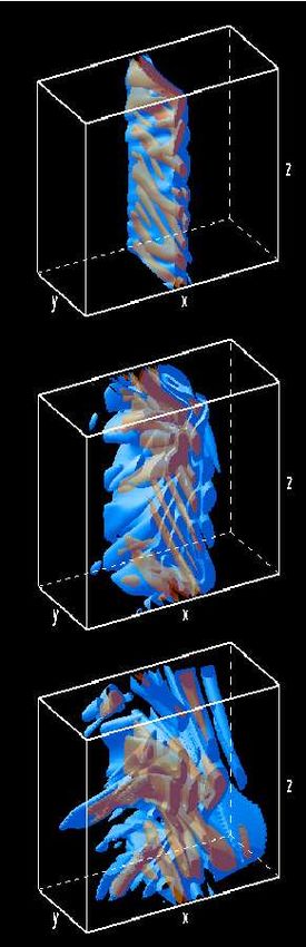
The nonlinear evolution of the system is characterized by the formation of
small scale structures, especially in the lateral regions of the computational
domain, and coalescence of magnetic islands in the center. This behavior is26 Loukas Vlahos, Sam Krucker and Peter Cargill
reflected in the 3-D structure of the current (see Fig. 16), which shows that
the initial equilibrium is destroyed by the formation of current filaments, with
a prevalence of small scale features. The final stage of these simulations is a
turbulent state, characterised by many spatial scales, with small structures
produced by a cascade with wavelengths decreasing with increasing distance
from the current sheet. In contrast, inverse energy transfer leads to the coa-
lescence of magnetic islands producing the growth of two-dimensional modes.
The energy spectrum approximates a power law with slope close to 2 at the
end of the simulation. Similar results have been reported by many authors
using several approximations [53, 119, 98, 154]. It is also interesting to note
that similar results are reported from magnetic fluctuations in the Earth’s
magnetotail [178].
Fig. 16. Current isosurfaces showing the formation of current filaments, [132]
It has become apparent over the years that the (theoretical) Ohm’s law
used in resistive MHD:
E + V × B = ηj (10)
where E and B are the electric and magnetic fields, V is the fluid velocity, j
is the current and η is the resistivity, breaks down near reconnection sites. The
main reason is that the region of electron demagnetization is much smaller
than the ion inertial length c/ωi , where c is the speed of light and ωi the ion
plasma frequency, and so Hall terms in the full version Ohm’s law become
important:
1 dj 1
= E+V ×B− j×B (11)
ωe2 dt neYou can also read