A MODEL FOR URBAN BIOGENIC CO2 FLUXES: SOLAR-INDUCED FLUORESCENCE FOR MODELING URBAN BIOGENIC FLUXES (SMURF V1) - GMD
←
→
Page content transcription
If your browser does not render page correctly, please read the page content below
Geosci. Model Dev., 14, 3633–3661, 2021
https://doi.org/10.5194/gmd-14-3633-2021
© Author(s) 2021. This work is distributed under
the Creative Commons Attribution 4.0 License.

A model for urban biogenic CO2 fluxes: Solar-Induced
Fluorescence for Modeling Urban biogenic Fluxes
(SMUrF v1)
Dien Wu1,a , John C. Lin1 , Henrique F. Duarte1,b , Vineet Yadav2 , Nicholas C. Parazoo2 , Tomohiro Oda3,4,5 , and
Eric A. Kort6
1 Department  of Atmospheric Sciences, University of Utah, Salt Lake City, UT, USA
2 NASA   Jet Propulsion Laboratory, California Institute of Technology, Pasadena, CA, USA
3 Goddard Earth Sciences Technology and Research, Universities Space Research Association, Columbia, MD, USA
4 Global Modeling and Assimilation Office, NASA Goddard Space Flight Center, Greenbelt, MD, USA
5 Department of Atmospheric and Oceanic Science, University of Maryland, College Park, MD, USA
6 Climate and Space Sciences and Engineering, University of Michigan, Ann Arbor, MI, USA
a now at: Division of Geological and Planetary Sciences, California Institute of Technology, Pasadena, CA, USA
b now at: Earth System Science Center, National Institute for Space Research, São José dos Campos, Brazil

Correspondence: Dien Wu (dienwu@caltech.edu)

Received: 8 September 2020 – Discussion started: 7 October 2020
Revised: 12 April 2021 – Accepted: 17 May 2021 – Published: 17 June 2021

Abstract. When estimating fossil fuel carbon dioxide            grained land cover classification in Los Angeles (r = 0.83).
(FFCO2 ) emissions from observed CO2 concentrations, the        Moreover, we compared SMUrF-based NEE with inventory-
accuracy can be hampered by biogenic carbon exchanges           based FFCO2 emissions over 40 cities and addressed the
during the growing season, even for urban areas where           urban–rural contrast in both the magnitude and timing of
strong fossil fuel emissions are found. While biogenic car-     CO2 fluxes. To illustrate the application of SMUrF, we used
bon fluxes have been studied extensively across natural veg-    it to interpret a few summertime satellite tracks over four
etation types, biogenic carbon fluxes within an urban area      cities and compared the urban–rural gradient in column CO2
have been challenging to quantify due to limited observa-       (XCO2 ) anomalies due to NEE against XCO2 enhancements
tions and differences between urban and rural regions. Here     due to FFCO2 emissions. With rapid advances in space-based
we developed a simple model representation, i.e., Solar-        measurements and increased sampling of SIF and CO2 mea-
Induced Fluorescence (SIF) for Modeling Urban biogenic          surements over urban areas, SMUrF can be useful to inform
Fluxes (“SMUrF”), that estimates the gross primary pro-         the biogenic CO2 fluxes over highly vegetated regions during
duction (GPP) and ecosystem respiration (Reco ) over cities     the growing season.
around the globe. Specifically, we leveraged space-based SIF,
machine learning, eddy-covariance (EC) flux data, and ancil-
lary remote-sensing-based products, and we developed algo-
rithms to gap-fill fluxes for urban areas. Grid-level hourly    1   Introduction
mean net ecosystem exchange (NEE) fluxes are extracted
from SMUrF and evaluated against (1) non-gap-filled mea-        Climate change and urbanization are two major worldwide
surements at 67 EC sites from FLUXNET during 2010–              phenomena in recent decades. In close connection with both
2014 (r > 0.7 for most data-rich biomes), (2) independent       themes, cities have attracted increasing attention from both
observations at two urban vegetation and two crop EC sites      researchers and policy makers. Urban ecosystems are unique
over Indianapolis from August 2017 to December 2018 (r =        and complex given the wide variety of land use and land
0.75), and (3) an urban biospheric model based on fine-         cover in cities, along with higher levels of atmospheric CO2

Published by Copernicus Publications on behalf of the European Geosciences Union.
3634                                                                   D. Wu et al.: A model for urban biogenic CO2 fluxes

concentration, air temperature, and vapor pressure deficit        (Miller et al., 2020; Turnbull et al., 2015). Carbonyl sulfide
than surrounding rural ecosystems (George et al., 2007).          (COS) shares a similar seasonal variation as CO2 over land
The consequences of climate change, such as severe heat,          as a result of biospheric sinks (Kettle et al., 2002). However,
drought, and water shortage events, may be particularly ex-       measurements of 14 C, COS, and CO2 fluxes are costly and
acerbated over (semi)arid and/or developing cities (Rosen-        lacking in most cities around the globe. Besides observa-
zweig et al., 2018), resulting in possible population move-       tions, many global terrestrial biospheric models provide in-
ment from increasingly hot and dry places to relatively cool      sights to inform and constrain CO2 fluxes at continental to
and moist ones. Meanwhile, rapid urban expansion and pop-         global scales (Huntzinger et al., 2013; Knorr and Heimann,
ulation growth contribute to the rise in total anthropogenic      2001; Philip et al., 2019), but their relatively coarse reso-
CO2 emissions into the atmosphere and the urban heat is-          lution and simplifications of the urban biosphere limit their
land, which further influences plant phenology (Meng et al.,      use for studying urban carbon cycles. Only a few biospheric
2020). Human activities have been continuously modifying          models are designed for simulating urban biogenic fluxes.
the urban and natural vegetation and soil, e.g., expansion of     Research has revealed urban–rural differences in vegetation
agricultural lands at the cost of the natural landscape, lead-    and soil properties, in part due to management strategies and
ing to less reversible ecological and climatic impacts (El-       environmental conditions, which complicate the flux quan-
lis and Ramankutty, 2008; Hutyra et al., 2014; Pataki et al.,     tification (Decina et al., 2016; Hardiman et al., 2017; Smith
2006). Hence, urban areas function as both biophysical and        et al., 2019; Vasenev and Kuzyakov, 2018). Among these few
socioeconomic systems, and studying their carbon sources          models, the urban Vegetation Photosynthesis and Respiration
and sinks facilitates understanding cities’ roles in the global   Model (urbanVPRM; Hardiman et al., 2017) is an empirical
carbon cycle.                                                     model that incorporates the urban heat island effect and im-
   To study the urban carbon pool and its exchange with the       pervious surface area into its flux calculations and currently
atmosphere, the top-down approach based on measured at-           uses conventional greenness indices, e.g., the enhanced veg-
mospheric CO2 concentrations is commonly used. McRae              etation index (EVI).
and Graedel (1979) noted over 4 decades ago that sepa-                Our work is primarily motivated by the relatively coarse
ration between anthropogenic and biogenic CO2 flux sig-           spatial grid spacing and the simplifications of urban ecosys-
nals is needed to interpret urban CO2 observations. Biogenic      tems in many models. We attempted to bridge the gap be-
CO2 fluxes are found to modify the surface CO2 and even           tween coarse-scale global biospheric models and highly cus-
atmospheric-column CO2 (XCO2 ) concentrations downwind            tomized local models to offer a global solution to modeling
(e.g., Lin et al., 2004; Turnbull et al., 2015; Hardiman et       biogenic CO2 fluxes within and around urban areas, which
al., 2017; Sargent et al., 2018; Ye et al., 2020). For exam-      would provide insight into CO2 partitioning between fossil
ple, the seasonal variation in biogenic CO2 signals in Los        fuel and biogenic components.
Angeles was found to be one-third of the observed annual              Thanks to advances in spaceborne and ground-based mea-
mean anthropogenic signal and further highlights the impor-       surements, solar-induced fluorescence (SIF) has been suc-
tance of urban irrigation (Miller et al., 2020). Over the Pearl   cessfully retrieved from various satellite platforms and has
River Delta in China, simulated biogenic contributions using      proven to be an effective proxy for photosynthesis and thus
15 different models in the Multi-scale Synthesis and Terres-      modeling gross primary production (GPP) (Frankenberg et
trial Model Intercomparison Project (MsTMIP; Huntzinger           al., 2011; Guanter et al., 2014; Joiner et al., 2013; X. Yang
et al., 2013) lead to downwind XCO2 anomalies ranging             et al., 2015). SIF tracks the unique seasonal and interan-
from nearly zero up to 1 ppm depending on seasons and mod-        nual variations in GPP across diverse plant functional types
els, which reveals the non-neglectable biogenic influence on      (PFTs) (Luus et al., 2017; Smith et al., 2018; Turner et al.,
XCO2 as well as the large inter-model uncertainty (Ye et al.,     2020; Zuromski et al., 2018) and their responses to phys-
2020). Thus, assessing the contributions from biogenic fluxes     iological stress (Magney et al., 2019). In an effort to im-
in observed signals is crucial for top-down estimates of urban    prove long-term, high-resolution spatial mapping capabil-
emissions yet remains challenging, especially given limited       ities, several spatially continuous SIF products have been
urban flux observations across the globe. Although decidu-        created using machine-learning (ML) techniques and light
ous trees are found to be the dominant tree type in urban areas   use efficiency modeling to combine satellite-retrieved SIF
based on a meta-analysis of 328 global cities (J. Yang et al.,    with ancillary vegetation data (Duveiller et al., 2020; Du-
2015), a more accurate approximation of the vegetation cov-       veiller and Cescatti, 2016; Li and Xiao, 2019a; Turner et
erages, types, and biological activities in cities is currently   al., 2021; Zhang et al., 2018). Moreover, the empirical and
hard to obtain.                                                   PFT-specific linear correlations between GPP and SIF, de-
   Existing approaches to separate biogenic and anthro-           rived from regressions of temporally aggregated (∼ monthly)
pogenic CO2 components involve the use of ancillary trac-         eddy-covariance GPP (Frankenberg et al., 2011; Guanter et
ers and terrestrial biospheric models. For instance, since ra-    al., 2014; Magney et al., 2019; Sun et al., 2017; Turner et
diocarbon (14 C) has decayed in fossil fuels, 14 C serves as      al., 2021; Zhang et al., 2018; Zuromski et al., 2018), have
a tracer for the combustion of fossil fuel (FF) emissions         spurred the development of upscaled GPP estimates (Li and

Geosci. Model Dev., 14, 3633–3661, 2021                                           https://doi.org/10.5194/gmd-14-3633-2021
D. Wu et al.: A model for urban biogenic CO2 fluxes                                                                        3635

Xiao, 2019b; Yin et al., 2020). SIF information has also been    2     Data and methodology
incorporated into existing process-based biospheric models
and data assimilation systems (MacBean et al., 2018; Van         SMUrF incorporates SIF as an indicator of photosynthesis,
Der Tol et al., 2009). Within the context of the urban bio-      along with possible drivers for Reco (i.e., air and soil temper-
sphere, SIF retrieved from space has been shown to reveal        atures and SIF-driven GPP), and performs hourly downscal-
the urban–rural gradient in photosynthetic phenology (Wang       ing using reanalysis-based temperature and radiation fields
et al., 2019). Given all these advantages, SIF would poten-      (Fig. 1). We accounted for variations in biome types and
tially benefit GPP estimates and CO2 flux partitioning over      Reco at 500 m before aggregating fluxes to the final grid spac-
cities.                                                          ing of 0.05◦ . Gridded uncertainties of daily mean fluxes are
   Ecosystem respiration (Reco ), the other component of net     quantified by assigning a biome-specific coefficient of vari-
ecosystem exchange (NEE), is defined as the sum of the au-       ation (CV) from model–data comparisons (Sect. 2.5). To
totrophic (RA ) and heterotrophic (RH ) components. In terms     gain insight into the column CO2 anomalies caused by an-
of modeling urban Reco , urbanVPRM follows the conven-           thropogenic and biogenic fluxes, we further adopted an at-
tional approach of VPRM (Mahadevan et al., 2008) to esti-        mospheric transport model to link fluxes and concentrations
mate an initial air-temperature-scaled (Tair -scaled) Reco and   (Sect. 2.6). Before introducing the steps for estimating indi-
splits Reco into equal components (RA and RH ) that will be      vidual flux components, we first go through the main input
further modified by considering impervious fractions and ur-     datasets (Sect. 2.1).
ban heat island effects (Hardiman et al., 2017). However, the
exact partitioning of Reco between RA and RH as well as the      2.1     Input datasets
separation between aboveground and belowground respira-
                                                                 Similar to many biospheric models, SMUrF estimates grid-
tion can be challenging and highly uncertain, as acknowl-
                                                                 ded GPP, Reco , and NEE (= Reco – GPP) fluxes based on
edged in Hardiman et al. (2017). The initial Reco that ur-
                                                                 land cover types. Main required data streams are summarized
banVPRM modified may be an overly simplistic function of
                                                                 in Fig. 1, including (1) the 500 m MODIS-based land cover
ambient air temperature. After all, the complexity of biolog-
                                                                 classification, (2) the 0.05◦ spatiotemporally contiguous SIF
ical and nonbiological processes of Reco and the lack of a
                                                                 (CSIF) product, (3) 100 m aboveground biomass (AGB) from
mechanistic understanding of how biotic and abiotic factors
                                                                 GlobBiomass, (4) eddy-covariance (EC) flux measurements
affect Reco render mechanistic modeling of Reco challeng-
                                                                 across continents, and (5) gridded products of air and soil
ing. Given the complexity in modeling Reco , we will turn
                                                                 temperatures.
instead to ML techniques that have been increasingly ap-
plied in many disciplines to help answer complicated, en-
                                                                 2.1.1    Land cover classification
tangled problems by extracting patterns from data streams
for predictions and generalizations. Reichstein et al. (2019)    Land cover classifications with more sophisticated algo-
provided a comprehensive review of the many applications         rithms in urban areas (e.g., NLCD 2016) are often avail-
of ML techniques in solving geoscience and remote sensing        able for limited regions. Thus, we adopted the land cover
problems and identified challenges in successfully adopting      types defined by the International Geosphere–Biosphere Pro-
ML approaches – e.g., interpretability, integration with phys-   gramme (IGBP) from MCD12Q1 v006 (Friedl and Sulla-
ical understanding and modeling, and the ability to cope with    Menashe, 2019) to inform biome types over global land.
model–data uncertainties. In the context of ecosystem mod-       The 12 biomes include croplands (CRO), closed and open
eling, an artificial neural network (NN) has been utilized to    shrublands (CSHR, OSHR), five types of forest (deciduous
generate SIF beyond satellite soundings (Li and Xiao, 2019a;     broadleaf – DBF, deciduous needleleaf – DNF, evergreen
Zhang et al., 2018), harmonize multiple SIF satellite instru-    broadleaf – EBF, evergreen needleleaf – ENF, mixed forests
ments (Wen et al., 2020), map carbon and energy fluxes (Tra-     – MF), grasslands (GRA), savannas (SAV), woody savannas
montana et al., 2016), and reveal and predict the trend in       (WSAV), and permanent wetlands (WET). Since MCD12Q1
global soil respiration (Zhao et al., 2017).                     simply treats the entire urban area as one category (URB), we
   In this paper, we present a model representation of GPP,      developed an algorithm to approximate the vegetation types
Reco , and NEE fluxes targeting urban areas around the globe,    and fractions in cities (Sect. 2.2.2).
the Solar-Induced Fluorescence (SIF) for Modeling Urban
biogenic Fluxes (“SMUrF”), by taking advantage of SIF and        2.1.2    Data for GPP estimates
the NN technique. Our main objectives include (1) examin-
ing the biogenic and anthropogenic CO2 fluxes and their tem-     We used the spatiotemporally contiguous SIF (CSIF; Zhang
poral variations over urban and surrounding rural areas and      et al., 2018) product and GPP fluxes from FLUXNET2015
(2) demonstrating one application of SMUrF to help inter-        (Pastorello et al., 2017) to calculate biome-specific GPP–
pret satellite CO2 observations by revealing the urban–rural     CSIF slopes (α, Fig. S1 in the Supplement). A total of 98
gradient in biogenic CO2 fluxes along satellite swaths of the    global EC tower sites with screened data points (quality flag
Orbiting Carbon Observatory 2 (OCO-2; Crisp et al., 2012).       < 3) from 2010 to 2014 are chosen to represent various

https://doi.org/10.5194/gmd-14-3633-2021                                            Geosci. Model Dev., 14, 3633–3661, 2021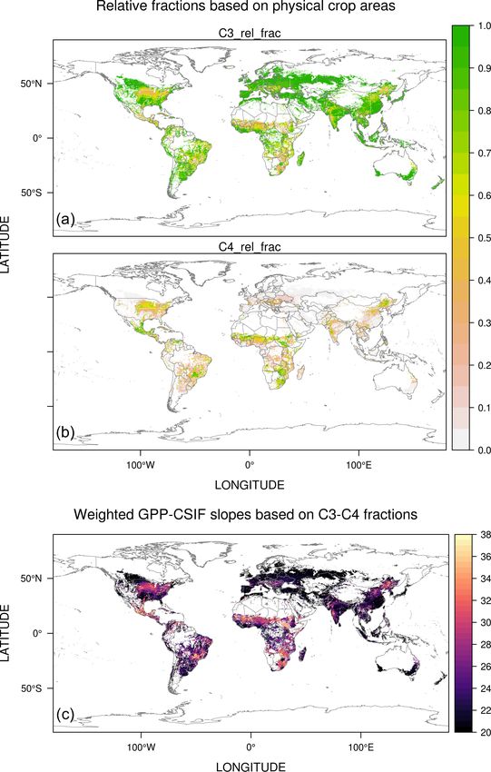
3636                                                                       D. Wu et al.: A model for urban biogenic CO2 fluxes

Figure 1. A demonstration of SMUrF (flowchart) and a description of input data products and observations (summarized in the table). The
temporal coverage in the table indicates the years used in this study.

biomes. CSIF offers global 4 d mean SIF at a grid spacing of          SIF retrievals from OCO-2 and GOME-2, considering the
0.05◦ during 2000–2018 using the NN approach (Zhang et                inevitable spatial mismatch between CSIF (0.05◦ ) and the
al., 2018). The NN model in CSIF is constructed based upon            direct sounding-level SIF measurements (OCO-2’s footprint
OCO-2 SIF and four broadband reflectances from MCD43C4                of ∼ 1 km × 2 km). The two largest biases of CSIF with re-
V006 under clear-sky conditions, and it is used for map-              spect to OCO-2 SIF arise from croplands (−12.72 %) and
ping SIF beyond sounding locations. CSIF agrees well with             urban areas (−14.59 %), caused by the saturation effect in

Geosci. Model Dev., 14, 3633–3661, 2021                                                https://doi.org/10.5194/gmd-14-3633-2021
D. Wu et al.: A model for urban biogenic CO2 fluxes 3637
broadband reflectances and built-up contamination in the re- 5 (ERA5, 0.25◦ ; Copernicus Climate Change Service Infor-
flectance signal, respectively (Zhang et al., 2018). To com- mation, 2017) for the entire globe or from Daymet (1 km;
pensate for the potential bias of urban CSIF, we scale up the Thornton et al., 2016) and the North American Land Data
GPP–SIF slope for urban areas (details in Sect. 2.2.2). Assimilation System (NLDAS; 0.125◦ ; Xia et al., 2012) as
In addition, the clear-sky instantaneous CSIF is com- alternative inputs for CONUS runs (Fig. 1). It is worth point-
pared to TROPOMI-based downscaled SIF for summer 2018 ing out that different models and reanalyses provide Tair at
(Turner et al., 2021) and vegetated fractions inferred from the 2 m above the ground but Tsoil at different soil depths. For
WUDAPT product (Appendix A). Despite some discrepan- instance, four soil depths from NLDAS are 10, 30, 60, and
cies over a few regions, these comparisons confirmed CSIF’s 100 cm below the ground, whereas ERA5 simulates mean
performance and capability in revealing the urban–rural gra- Tsoil over four vertical layers, i.e., 0–7, 7–28, 28–100, and
dient in biogenic activities (Figs. S2–S3). 100–289 cm. Measured soil depths from FLUXNET are even
more complicated and vary among sites, with the most com-
2.1.3 Data for approximation of urban vegetation mon shallowest soil depth at ∼ 2 cm below the ground. To
globally reconcile differences in soil depths, we chose measured Tsoil
from the shallowest layer in both the model and observational
To assign trees and grass within the MODIS-based urban do- datasets to separately build NN models (Sect. 2.3).
main, several steps are carried out to approximate the relative
fractions of (1) tree versus non-tree, (2) individual tree types, 2.1.5 Data for flux comparisons
and (3) grassland versus shrubland (details in Sect. 2.2.2).
Relative tree fractions (i.e., ratio of tree fractions to total veg- We further carried out flux comparisons against two inde-
etated fractions) can be obtained from two data sources: a pendent sets of eddy-covariance data, i.e., FLUXNET2015
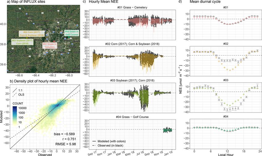
0.6 m urban land cover product (Coleman et al. 2020) based and the Indianapolis Flux Experiment (INFLUX; Davis et
on the National Agriculture Imagery Program (NAIP) and al., 2017; K. Wu, 2020), and one alternative urban biospheric
a 250 m vegetation continuous field (VCF) from MOD44B model (urbanVPRM) over Los Angeles in Sect. 3.2. Only
(Dimiceli et al., 2015). Both products offer estimated tree non-gap-filled measured NEE fluxes from FLUXNET2015
and vegetated fractions. The former one is produced only (with a quality flag of 0) are used for validation. Since NEE
over Los Angeles via random forest algorithms that trained fluxes measured from INFLUX have not been gap-filled, we
on Sentinel-2 (∼ 5 m) and NAIP (∼ 0.6 m) optical imagery only chose the hours from SMUrF when valid INFLUX data
(Coleman et al., 2020), and it possesses much higher tree are available.
fractions than MODIS VCF (see comparisons in Sect. 2.2.2). The INFLUX project includes EC flux measurements that
Thus, we decided not to utilize MODIS VCF for indicating accompany the tower- and aircraft-based greenhouse gas
urban vegetation in this work, only for comparing tree frac- (GHG) mole fraction measurements. These sites have been
tions from Coleman et al. (2020). periodically moved to sample different components of the
To approximate relative tree fractions (ftree ) in cities, we urban landscape. For the period from 10 August 2017 to
treat the gridded AGB at 100 m from GlobBiomass (San- 7 June 2019, these flux towers were deployed at two urban
toro et al., 2018) as the spatial proxy (see the methodology vegetation sites (no. 1 and no. 4) and two agricultural sites
explanation in Sect. 2.2.2). GlobBiomass deployed a com- (no. 2 and no. 3). Two urban vegetation (turf grass) sites were
plex retrieval algorithm system that involves a series of re- located in a cemetery area (site no. 1) and on a golf course
trieval algorithms using radar backscatter and several other (site no. 4). Because CSIF is not available beyond 2018 at
data types such as laser measurements from ICESAT (Schutz the time of writing, we cannot yet extend the flux compari-
et al., 2005), tree and land cover data (e.g., from Landsat), son into 2019. Fluxes from INFLUX sites were computed us-
and collections of reanalyses and models. AGB and its grid- ing EddyPro software (LI-COR Biosciences, 2012) and post-
level uncertainty [t ha−1 ] by definition describe the “oven- processed to filter out data when (a) the LI-COR gas analyzer
dry weight of the woody parts (stem, bark, branches, and signal strength was low and (b) during periods of weak tur-
twigs) of all living trees excluding stump and roots” (San- bulence (K. Wu, 2020). It is worth noting that INFLUX data
toro et al., 2018). GlobBiomass AGB has demonstrated good provide valuable independent evaluations as flux sites with
agreement with independent data products for different con- an urban imprint are lacking from FLUXNET2015, and ob-
tinents (Santoro et al., 2018). served fluxes from INFLUX sites were not used when cali-
brating parameters in SMUrF.
2.1.4 Reanalyses for Reco estimates The urbanVPRM, applied over Los Angeles, estimates
GPP from a light use efficiency modeling perspective
In an effort to train and predict Reco via neural network mod- driven by reanalysis-based photosynthetically active radia-
els, we chose GPP as well as air and soil temperatures (Tair tion (PAR) as well as the satellite-derived EVI and land sur-
and Tsoil ) as explanatory variables (details in Sect. 2.3). Mod- face water index (LSWI) for phenology and water availabil-
eled Tair and Tsoil are taken from the ECMWF ReAnalysis- ity. It estimates Reco via an air temperature function with ex-
https://doi.org/10.5194/gmd-14-3633-2021 Geosci. Model Dev., 14, 3633–3661, 2021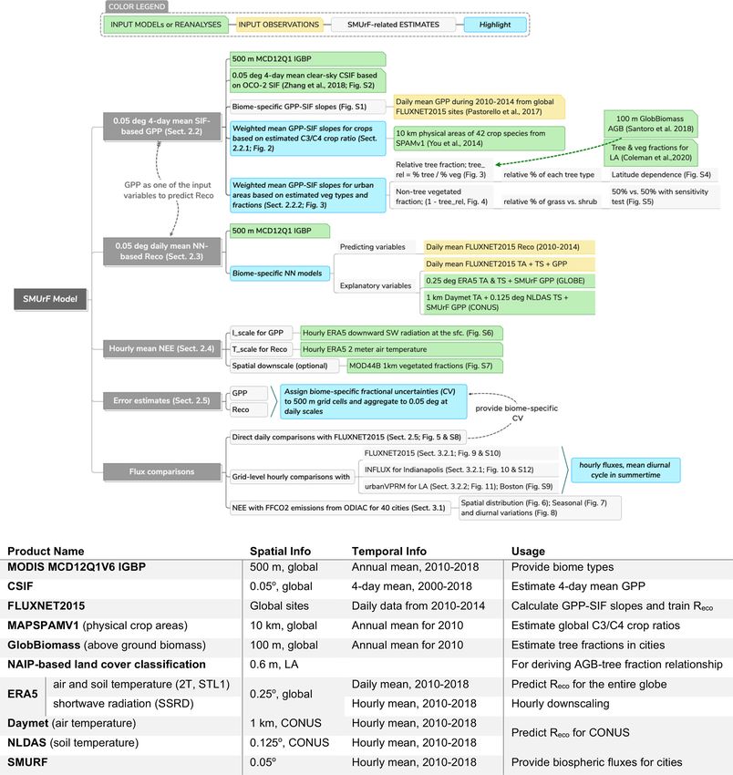
3638                                                                  D. Wu et al.: A model for urban biogenic CO2 fluxes

tra modifications to air temperature due to the urban heat is-
land effect and impervious surface area. The urbanVPRM-
based fluxes rely on the 60 cm NAIP-based land cover clas-
sification in Los Angeles (Coleman et al., 2020; Sect. 2.1.3).
Due to differences in grid spacing between models, fluxes
from urbanVPRM are aggregated and re-projected from 30 m
to 0.05◦ to match SMUrF for the purposes of comparison.

2.2     GPP estimates

We used 4 d mean clear-sky SIF from CSIF and 4 d mean ob-
served GPP fluxes from 98 global eddy-covariance (EC) tow-
ers from FLUXNET2015 to derive biome-specific GPP–SIF
slopes (α, Fig. S1) with special treatments to α over crop-
lands and urban areas, as described in the following subsec-
tions. While nonlinear relationships between SIF and GPP at
leaf and canopy level have been observed (Helm et al., 2020;
Magney et al., 2017; Maguire et al., 2020; Marrs et al., 2020;
Verma et al., 2017), GPP is observed to be linearly related
to SIF at increasing temporal and spatial (ecosystem and re-
gional) scales (Frankenberg et al., 2011; Sun et al., 2017) as
leaf-level differences in composition, light exposure, stress,
and stress response mix out (Magney et al., 2020). Consid-
ering uncertainty in CSIF and flux-tower-partitioned GPP as
well as the noise in the GPP–SIF relationship across global
flux sites (Fig. S1), we adopted linear fits instead of nonlin-
ear fits between GPP and CSIF. Errors due to departure from
linearity will be implicitly included in GPP uncertainties cal-
culated from model–tower validations (Sect. 2.5). The calcu-
lated α values are in proximity to those reported in Zhang
et al. (2018) from 40 towers and are assigned to each 500 m
grid cell according to the corresponding biome type.

2.2.1    C3 / C4 partitioning of croplands                        Figure 2. Spatial distribution of the estimated C3 : C4 ra-
                                                                  tio [%] (a–b) using physical areas of 42 crop species
                                                                  from MapSPAMv1 and weighted mean GPP–CSIF slopes
GPP–SIF relationships differ between C4 and C3 crops at           [(µmol m−2 s−1 )/(mW m−2 nm−1 sr−1 )] for croplands (c).
the canopy scale, since GPP for C3 crops may saturate at
high PAR levels. Different statistical fits between observed
GPP and SIF are suggested for C3 versus C4 crops (He et           weighted mean α according to the C3 : C4 ratio map and
al., 2020). Despite the focus of SMUrF on urban areas, we         identified tropical regions, the midwestern US, northeastern
still attempted to differentiate C4 from C3 crops and esti-       China, and spots in India and southern Africa as regions
mate two different α values from EC sites dominated by            with higher α and C4 crop ratios (Fig. 2c). Note that these
C3 or C4 crops. Specifically, the Spatial Production Alloca-      weighted mean α values will only be activated over MODIS-
tion Model (SPAM 2010V1.1; You et al., 2014) is used for          based croplands.
areal estimates of 42 crop species, among which the follow-
ing are identified as C4 crops: maize, pearl and small millet,    2.2.2   Modification to urban vegetation
sorghum, and sugarcane. As a result, we produced maps of
C3 : C4 ratios at a grid spacing of 10 km for the entire world    We next turn to the estimate of α over the MODIS-based
(Fig. 2a, b). Four of the selected 13 cropland EC FLUXNET         “urban” category shown in the following three steps (Fig. 1).
sites fall within grid cells with a high C4 ratio of > 50 %;
the remaining sites fall into grid cells with C4 ratios of         1. Estimate the relative tree fraction (ftree =
< 10 %. We thereby arrive at αC4 of ∼ 35.6 [µmol m−2 s−1 ] :          tree / vegetation). A power-law relationship (Fig. 3a)
[mW m−2 nm−1 sr−1 ] from sites with a high C4 ratio and               between AGB bins and relative tree fractions obtained
αC3 of ∼ 19.7 [µmol m−2 s−1 ] : [mW m−2 nm−1 sr−1 ] from              from the NAIP-based land cover classification (top
the other nine cropland sites. Eventually, we calculated the          panel in Fig. 3b) is used to predict ftree (bottom panel in

Geosci. Model Dev., 14, 3633–3661, 2021                                           https://doi.org/10.5194/gmd-14-3633-2021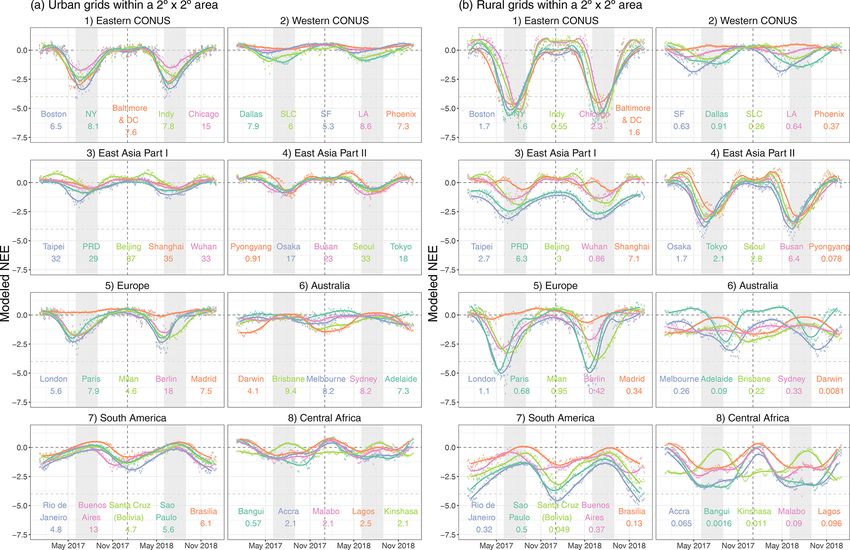
D. Wu et al.: A model for urban biogenic CO2 fluxes                                                                                         3639

Figure 3. (a) Power-law relationships fitted between the aboveground biomass (AGB) and raw relative tree fractions (purple line) as well as
fits using binned AGB and mean or median relative tree fractions per AGB bin (green or blue lines). The statistical fit in purple is chosen
to predict relative tree fractions within cities. (b) Spatial distributions of calculated relative tree fractions (%) from a high-resolution NAIP-
based land cover classification product (Coleman et al., 2020) (top panel), vegetation continuous fields from the MOD44B v6 product (middle
panel), and our approximation (bottom panel) using AGB and the statistical fit illustrated in panel (a).

     Fig. 3b). Although the AGB binning procedure may not                     3. Calculate weighted mean α. The α values for urban ar-
     fully recreate the variations in ftree , especially for grid                eas are weighted mean values calculated from biome-
     cells with zero AGB (dark red hexagons in Fig. 3a),                         specific α values and their corresponding fractions ap-
     the predicted ftree using AGB is tied to a smaller bias                     proximated in step 2. To account for the potential nega-
     of +2.3 % than ftree using MOD44B (−23.5 %) when                            tive bias of ∼ 14.5 % in CSIF over cities (Zhang et al.,
     the high-resolution NAIP-based land cover product is                        2018), we scaled up urban α by 1.145.
     compared (Fig. 3b).
                                                                           In the end, α values at 500 m over urban and natural lands
  2. Estimate relative fractions of five tree types, grass, and            (third row in Fig. 4) are aggregated to 0.05◦ and multiplied
     shrubs based on climatology. Due to the lack of global                by CSIF to arrive at GPP at 0.05◦ . The exact partitioning be-
     data on urban biome types, the relative non-tree vege-                tween grass and shrub in step (2) plays a minor role in the
     tated fraction (fnon-tree = 1 − ftree ) is simply split into          final GPP flux at 0.05◦ (Fig. S5). It is worth clarifying that
     half grass and half shrub (second row in Fig. 4). The                 we implicitly assumed that vegetation “exists” over urban
     relative tree fractions are divided into five possible tree           grid cells and only solved for the relative tree versus grass
     types (i.e., DBF, DNF, EBF, ENF, MF). The share of                    fractions as illustrated in steps (1) and (2), as information
     each tree type in cities is approximated as a function of             on vegetated and impervious fractions has been embedded
     latitude based on the climatology of land cover types                 in the CSIF product. Additional information about vegetated
     (Fig. S4a), e.g., high fractions of ENF over high lati-               and impervious fractions was not necessary in the calcula-
     tudes, EBF over tropical lands, and DBF plus MF over                  tion of α for every 500 m urban grid (see Appendix A for a
     the midlatitudes (Fig. S4b).                                          further explanation).

https://doi.org/10.5194/gmd-14-3633-2021                                                        Geosci. Model Dev., 14, 3633–3661, 2021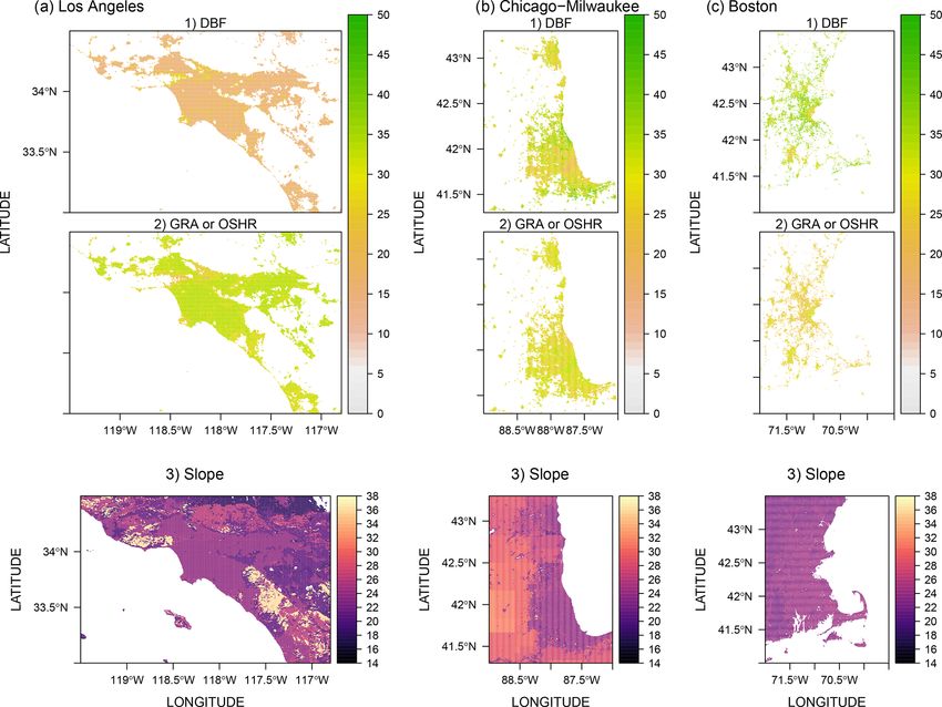
3640                                                                          D. Wu et al.: A model for urban biogenic CO2 fluxes

Figure 4. Estimated relative deciduous broadleaf forest (DBF, first row) and non-tree fractions (fnon-tree , second row) at 500 m as well as
GPP–SIF slopes after urban gap filling (third row) for Los Angeles (a), Chicago (b), and Boston (c).

2.3    Reco estimates                                                   NN models for C3 and C4 crops and calculated the weighted
                                                                        mean Reco based on the derived C3 : C4 ratios. 80 % and 20 %
Three explanatory variables – Tair , Tsoil , and GPP – are              of the data points per biome are used for training and testing,
chosen to train against the observed daily mean Reco from               respectively. Models with two hidden layers are constructed
FLUXNET. To account for mismatches in reported soil                     with 32 and 16 neurons chosen for the first and second layer.
depths (introduced in Sect. 2.1.4), we built separate sets of           We computed Reco at 500 m by applying biome-specific
NN models using (1) direct temperatures and GPP obser-                  models and aggregated those Reco to 0.05◦ . We also tested
vations from EC towers, (2) ERA5-based temperatures and                 two alternative ways to train Reco based on (1) all data points
SIF-based GPP, or (3) Daymet and NLDAS-based temper-                    without differentiating their land cover types and (2) addi-
atures and SIF-based GPP (only for the US as alternative                tional categorical variables from biomes and the month and
runs). SIF-based GPP is ingested in order to pass SIF infor-            season of the year. Please refer to Appendix B for sensitivity
mation on to Reco estimation. Data points from a few EC                 tests and technical details about data preparation and cross-
sites with relatively large uncertainties in modeled GPP were           validation of neural networks.
excluded before the training of NN models to prevent error
propagation into Reco (Appendix B).                                     2.4    NEE estimates
   For each set of NN models, we manually split data points
based on their biome types and obtain 12 separate NN mod-               We obtained hourly surface downward shortwave radiation
els. Data points from open and closed shrublands are com-               (SWrad ) and air temperature (Tair ) from the ERA5 reanaly-
bined due to the extremely low numbers of EC sites around               sis to calculate the hourly scaling factors for GPP and Reco .
the globe. To be consistent with the C3 : C4 crop partition             Tair and SWrad are initially provided at a grid spacing of
for GPP estimates (Sect. 2.2.1), we obtained two separate               0.25◦ and then bilinearly interpolated to 0.05◦ . To estimate

Geosci. Model Dev., 14, 3633–3661, 2021                                                   https://doi.org/10.5194/gmd-14-3633-2021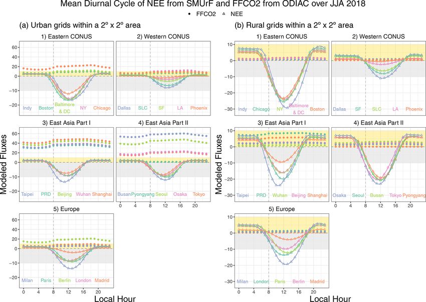
D. Wu et al.: A model for urban biogenic CO2 fluxes                                                                            3641

the hourly radiation scaling factors Iscale for GPP, we nor-          flux tower location and directly computed the modeled GPP
malized the hourly SWrad by the 4 d mean SWrad with the               and Reco using α values and NN models. Comparisons be-
same time window of the 4 d mean GPP. Regarding the cal-              tween these direct computations and screened observations
culation of hourly temperature scaling factors Tscale for Reco ,      from FLUXNET2015 yield biome-specific root mean square
a temperature sensitivity function (SR1 h ) has been modified         errors (RMSEs), mean biases, and CVs. The uncertainties in
from prior studies (Fisher et al., 2016; Olsen and Randerson,         assuming a linear GPP–SIF relationship were not explicitly
2004):                                                                quantified but incorporated within these error statistics on
              Tair,1 h −30 ◦ C
                                                                      top of other error sources such as inter-site variations. Even-
SR1 h = Q10        10 ◦ C        ,                              (1)   tually, biome-specific CVs are assigned to each 500 m grid
                                                                      and aggregated to 0.05◦ assuming statistical independence.
where Q10 is a unitless temperature sensitivity parameter that        For visualization purposes, we collected model–data pairs re-
could vary across biomes, and Tair is in degrees Celsius (◦ C).       gardless of their biome types as density plots in Fig. 5.
Because the hourly downscaling procedure is performed on                 Directly computed 4 d mean GPP values at most tow-
GPP and Reco fluxes at 0.05◦ and no single biome is tied to           ers match observations well regarding their magnitude and
each 0.05◦ grid cell, we adopt a typical Q10 value of 1.5 ac-         seasonality. Modeled GPP shows underestimations against
cording to previous studies (Fisher et al., 2016) despite pos-        irrigated maize sites in Nebraska (e.g., US-Ne1, US-Ne2)
sible biome-dependent variations in Q10 . SR1 h is then nor-          and sites in the Central Valley (e.g., US-Twt) in California
malized by its daily mean value to obtain Tscale . Finally, Tscale    (Fig. S8), likely because the irrigation effect is not explic-
and Iscale are used to temporally downscale the daily mean            itly included, and high crop chlorophyll concentrations may
Reco and 4 d mean GPP, i.e., Reco,1 d and GPP4 d .                    not be fully recreated in the reflectance-driven CSIF data.
                                                                      Nevertheless, the overall correlation coefficient between di-
                                                SR1 h                 rectly modeled GPP and partitioned GPP from FLUXNET
Reco,1 h = Reco,1 d · Tscale = Reco,1 d ·    1 P
                                             24    SR1 h              is 0.86, with a mean bias of −0.069 µmol m−2 s−1 for 89
                                                1d
                                                                      tower sites. When removing cropland sites from consid-
                                                SWrad,1 h             eration, the RMSE in 4 d mean GPP drops from 1.91 to
GPP1 h = GPP4 d · Iscale = GPP4 d ·          1 P
                                                                (2)
                                            24·4    SWrad,1 h         1.74 µmol m−2 s−1 (Fig. 5a vs. b).
                                                 4d                      Next, we report the predicting performance of Reco only
Examples of Iscale and Tscale over the western US on                  using testing sets, i.e., 20 % of the entire data volume. Reco
2 July 2018 are displayed in Fig. S6bc. As a sanity check             values trained and predicted using measured variables from
for the ERA-based SWrad , a higher-resolution product is uti-         FLUXNET overperform the ones using ERA5’s tempera-
lized, from which SWrad and PAR were estimated based on               tures and SIF-modeled GPP (r = 0.90 vs. r = 0.87; Fig. 5c
Earth Polychromatic Imaging Camera (EPIC, on board the                vs. d). The constant CSIF within a 4 d interval and the con-
Deep Space Climate Observatory – DSCOVR) data and ran-                stant α over seasons make it difficult to reproduce daily
dom forest algorithms (Hao et al., 2020a, b). The EPIC-based          variations in Reco as Tair and Tsoil likely become the main
radiation data are available globally at 10 km from June 2015         drivers. Recall that temperature fields from higher-resolution
to June 2019 and have been validated against in situ observa-         Daymet + NLDAS were also used for training and pre-
tions from the Baseline Surface Radiation Network and Sur-            dicting Reco over CONUS. These Daymet + NLDAS runs
face Radiation Budget Network. Hourly Iscale values using             appear to slightly outperform the ERA5 runs (Fig. 5g vs.
ERA5-based SWrad and EPIC-based SWrad or PAR gener-                   f). Although the NN model using observed variables yields
ally agree well regarding the diurnal cycles, despite small           the best performance, we are inclined to use NN models
discrepancies in peak radiation and Iscale values during noon         trained by modeled features for two reasons: (1) to account
hours (Fig. S6de).                                                    for discrepancies in GPP and temperature between tower
                                                                      observations and models and/or reanalyses and (2) for spa-
2.5   Uncertainty quantification and direct flux                      tial generalization beyond points with “ground truth” as
      validation                                                      only modeled GPP is available away from the EC sites.
                                                                      Nevertheless, the mean bias in testing sets across biomes
Error quantification is important for characterizing the pre-         remains small (< 10−3 µmol m−2 s−1 ), with an RMSE of
cision and accuracy of modeled fluxes. Previous studies               1.14 µmol m−2 s−1 . Since the error statistics associated with
have carried out comprehensive uncertainty estimates to-              the ERA5 runs resemble those with the Daymet + NLDAS
wards their reported biogenic flux estimates (Dietze et al.,          runs over the US (Fig. 5f vs. g), we only present the ERA5-
2011; Hilton et al., 2014; Lin et al., 2011; Xiao et al., 2014).      based results in the following sections.
Here we estimated errors in modeled GPP and Reco based on                An additional hourly mean NEE evaluation against
FLUXNET observations.                                                 FLUXNET can be found in Sect. 3.2.1 and Fig. 9. We stress
   We extrapolated the biome type, 4 d mean SIF, and daily            that the directly computed fluxes and the validation with
mean Tair and Tsoil from their original gridded fields to each        FLUXNET presented in this section differ from those pre-

https://doi.org/10.5194/gmd-14-3633-2021                                                Geosci. Model Dev., 14, 3633–3661, 2021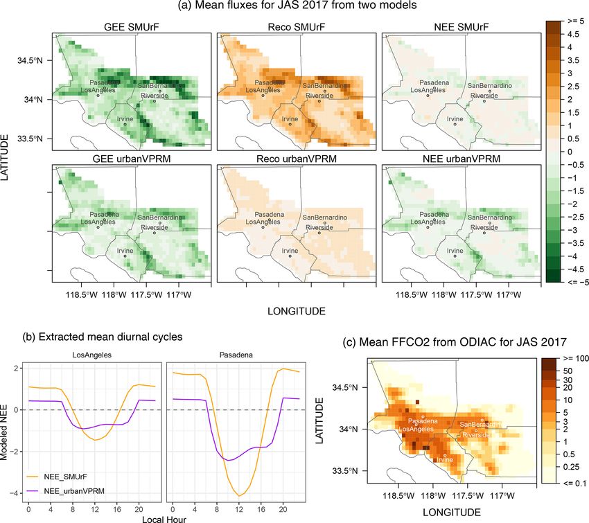
3642 D. Wu et al.: A model for urban biogenic CO2 fluxes
Figure 5. Comparisons between directly computed fluxes from SMUrF and observed fluxes from FLUXNET during 2010–2014 as density
plots with 50 bins. All fluxes have units of µmol m−2 s−1 . (a–b) 4 d mean observed GPP and directly computed SIF-based GPP at 89 global
EC sites (a) and 78 non-crop sites (b). (c–d) An evaluation of the daily mean observed Reco and predicted Reco in the testing set (i.e., 20 %
of all data) using observed Tair + Tsoil + GPP from FLUXNET (c) or Tair + Tsoil from ERA5 and SIF-based GPP (d) for 89 global EC sites.
(e–g) Similar to panels (c)–(d), but the model–data Reco comparison only for US EC sites and modeled Reco is calculated using Daymet Tair ,
NLDAS Tsoil , and SIF-based GPP (g). Although GPP and Reco were trained and predicted separately per biome, model–data pairs from all
biomes are collected for visualization purposes. For each panel, numbers of data points in each of the 50 bins are displayed in log10 scales
as yellow–blue colors, and error statistics including the mean bias, correlation coefficient, and RMSE are printed. The 1 : 1 and ordinary-
least-square-based (OLS-based) regression lines are displayed as solid and dashed lines. RMSEs derived from these direct validations were
further used for assigning uncertainties at the 500 m grid cell (Sect. 2.5).
sented in Sect. 3.2.1, as the latter one uses the spatially use of an atmospheric transport model – i.e., the column
weighted mean flux at 0.05◦ that takes the spatial heterogene- version of the Stochastic Time-Inverted Lagrangian Trans-
ity into account. port (X-STILT; Wu et al., 2018) model. We carried out
four case studies by examining summertime OCO-2 tracks
2.6 Comparisons of FFCO2 vs. NEE fluxes and their over Boston, Indianapolis, Salt Lake City, and Rome. Those
contributions to column CO2 four cities are chosen based on satellite data availability and
quality as well as various vegetation coverages. Specifically,
FFCO2 emissions from the Open-Data Inventory for Anthro- thousands of air parcels are released in STILT (Fasoli et al.,
pogenic Carbon dioxide (ODIAC2019; Oda et al., 2018) are 2018; Lin et al., 2003) from the same atmospheric columns
compared against NEE from SMUrF in terms of the sea- as the OCO-2 soundings and driven by meteorological fields,
sonal magnitude, summertime diurnal cycle, and spatial dis- i.e., the 3 km High-Resolution Rapid Refresh (HRRR) for
tribution (Sect. 3.1). Initial ODIAC emissions at 1 km grid US cities and 0.5◦ GDAS for non-US cities (Rolph et al.,
spacing are averaged to 0.05◦ for such FFCO2 –NEE com- 2017). The X-STILT model returns hourly surface influence
parisons. Although the city-wide FFCO2 emissions from matrices or “column footprints” [ppm/(µmol m−2 s−1 )] that
ODIAC may differ from other reported emissions (Chen et incorporate the averaging kernel and pressure weighting pro-
al., 2020; Oda et al., 2019), ODIAC is widely used in many files from OCO-2. The hourly footprints indicate the influ-
urban studies and provides sufficient insights into FFCO2 ence of each upwind grid cell on downwind satellite sound-
emissions from a global perspective. ings within each hour interval. The coupling between col-
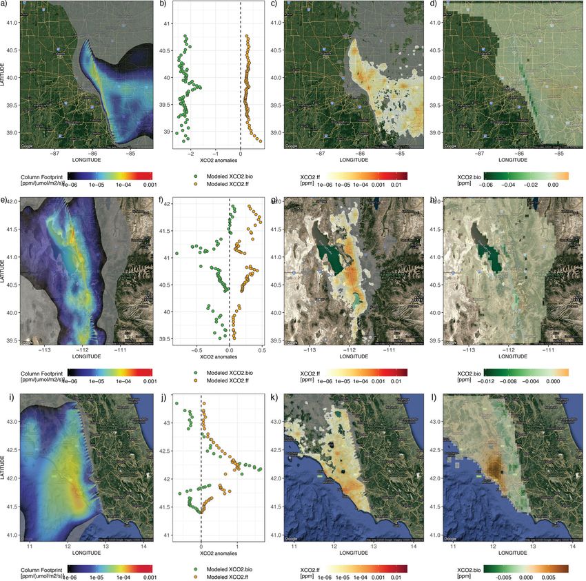
To further translate CO2 fluxes into changes in column- umn footprints and surface fluxes, e.g., hourly SMUrF-based
averaged CO2 concentrations, or XCO2 (Sect. 3.3), we made
Geosci. Model Dev., 14, 3633–3661, 2021 https://doi.org/10.5194/gmd-14-3633-2021D. Wu et al.: A model for urban biogenic CO2 fluxes 3643
NEE or ODIAC-based FFCO2 emissions, reveals (1) the spa- rate of soil respiration approaching FFCO2 emissions in a
tially explicit XCO2 contribution [ppm] due to biogenic and residential area and forest to the west of an urban core. Yet,
anthropogenic fluxes and (2) the overall XCO2 anomalies when it comes to interpreting observed CO2 concentrations,
(XCO2.bio , XCO2.ff ) at each receptor if the aforementioned it is the net flux that should be compared against FFCO2 .
spatial contributions are summed up. For more details on In short, biogenic fluxes have the potential to dominate the
ODIAC and X-STILT, please refer to Oda et al. (2018) and overall carbon flux exchange over residential and rural areas,
Wu et al. (2018), respectively. while FFCO2 is the main controller within urban cores.
We further extend the analysis to 40 cities across multi-
ple continents to see how CO2 fluxes vary between (1) ur-
3 Results ban and adjacent rural areas, (2) different cities, (3) the FF
and NEE components, and (4) across seasons. Specifically,
We start with modeled biogenic and anthropogenic fluxes at FFCO2 and NEE fluxes are averaged over urban and rural
the regional and urban scales (Sect. 3.1) as well as their com- grid cells within a 2◦ × 2◦ region around city centers. Here
parisons against EC observations and urbanVPRM over natu- urban grids are simply defined as the “urban and build-up set-
ral biomes and urban areas (Sect. 3.2). For the purpose of this tlements” according to MCD12Q1, while rural grids contain
paper gridded fluxes were produced from 1 January 2017 to all the natural counterparts (e.g., forests, grasslands, crop-
31 December 2018 only for the following populated and veg- lands) except for water, ice, and barren lands. In particular,
etated regions: CONUS, western Europe, East Asia, South we are interested in the seasonal variation (Sect. 3.1.1) and
America, central Africa, and eastern Australia. mean summertime diurnal cycle (Sect. 3.1.2) of these urban
and rural fluxes. The diurnal cycles of FFCO2 are calculated
3.1 Biogenic and anthropogenic CO2 fluxes at the using hourly scaling factors from Temporal Improvements
regional and city scale for Modeling Emissions by Scaling (TIMES; Nassar et al.,
2013) on top of monthly mean ODIAC-derived emissions.
To reveal the role of biospheric fluxes in the context of an- Note that emission temporal patterns provided by TIMES are
thropogenic emissions, we summed up NEE from SMUrF climatological, based on a US gridded inventory by Gurney
and FFCO2 emissions from ODIAC for each season over et al. (2009), and thus do not change in response to local en-
CONUS, western Europe, and East Asia (Fig. 6a, b, c). vironmental conditions, such as air temperature.
SMUrF reveals the spatial contrasts and seasonal variations
in NEE fluxes, as informed by the use of SIF, land cover 3.1.1 Seasonal variation
types, and temperature fields. Places with a strong seasonal
amplitude are found to be rural regions covered by crops and Stronger net biospheric uptake during growing seasons and
dense forests, e.g., the eastern US, northeastern and southern a larger seasonal amplitude in NEE are more linked to ru-
China, and spotty locations over Europe (green shading ar- ral grids than to urban grids as expected (Fig. 7a vs. b).
eas in Fig. 6a, b, c). After adding FFCO2 emissions, the sum Among the selected 40 cities, the top “wet” biologically ac-
of NEE and FFCO2 remains positive over East Asia even in tive cities include Boston, Baltimore and DC, New York,
summer months (“brownish” spots in Fig. 6c). Taipei, London, Paris, and Rio de Janeiro. By contrast, a
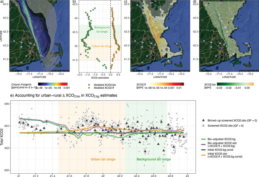
We next zoom into fluxes at the city scale. SMUrF captures few “drier” cities stand out, with the spatially averaged NEE
the increasing biospheric activities from urban cores to their over urban grids close to zero, such as Los Angeles, Phoenix,
rural surroundings inferred by gross ecosystem exchange and Madrid (Fig. 7a). Besides NEE magnitude, cities reach
(GEE is −GPP), Reco , and NEE components (eight zoomed- their maximum net uptake at different times: e.g., June–July
in panels in Fig. 6), as cities are usually associated with less for most cities in the eastern US and East Asia (except for
vegetation coverage than their rural counterparts. The urban– Taipei); a slightly earlier peak for most cities in the western
rural difference in GEE over Salt Lake City, Boston, and US, western Europe, and Taipei; and January for cities in the
Seoul is relatively small, in contrast to cities like Guangzhou Southern Hemisphere. For instance, minimum NEE is found
and Tokyo. Since modeled Reco is partially driven by SIF- in late May to June within and around London (Fig. 7a5),
based GPP, the spatial variations of GEE and Reco appear which is consistent with the seasonality of the posterior NEE
alike to some extent. Even though GPP can be high over fluxes reported for the UK from 2013 to 2014 (White et al.,
JJA 2018, summertime mean NEE remains small at urban 2019).
cores, with values ranging from −1 to −2 µmol m−2 s−1 . Since FFCO2 emissions fluctuate less across seasons than
For Boston, the spatial distribution of GEE and Reco derived NEE, we compare the magnitude of the seasonal amplitude
from SMUrF (Fig. 6) resembles what was reported using of NEE relative to the annual mean FFCO2 emission (shown
urbanVPRM (Fig. 2c in Hardiman et al., 2017). Reco from as numbers below city names in Fig. 7). Such a compar-
SMUrF exceeds ODIAC-based FFCO2 emissions over resi- ison helps inform the potential interference from the bio-
dential and rural areas away from urban cores (Fig. 6), which sphere over cities when interpreting long-term CO2 obser-
coincides with Decina et al. (2016), who reported an elevated vations, albeit without considering the atmospheric trans-
https://doi.org/10.5194/gmd-14-3633-2021 Geosci. Model Dev., 14, 3633–3661, 20213644 D. Wu et al.: A model for urban biogenic CO2 fluxes
Figure 6. The sums of seasonal mean SMUrF-based NEE and ODIAC-based FFCO2 [µmol m−2 s−1 ] for CONUS (a), western Europe (b),
and East Asia (c) at 0.05◦ for 2018. Spatial distributions of the average GEE (−GPP), Reco , NEE, and FFCO2 from ODIAC over JJA 2018
are provided for eight cities (hereinafter zoomed-in panels). As an optional step, these fluxes can further be spatially downscaled to 1 km
using MOD44B (Fig. S7).
port and the fact that the one single number for FFCO2 can during noon hours in summer months. For instance, the
be affected by large point-source emissions. As expected, peak value of summertime average NEE and FFCO2 fluxes
most spatially averaged FFCO2 emissions over urban grids over Boston is about −16 and 10 µmol m−2 s−1 , respectively
are stronger than the seasonal amplitude of NEE (Fig. 7a). (Fig. 8a1), at the hourly scale.
Exceptions include Pyongyang and cities in central Africa With regard to the timing of hourly fluxes, NEE in most
whose seasonal NEE amplitudes approach their annual mean midlatitude cities starts to dip below zero at 07:00 or 08:00
FFCO2 emissions, e.g., 2.0 vs. 2.5 µmol m−2 s−1 for La- local time (Fig. 8a), which is slightly later than the typical
gos. Things can get more complex if one tries to interpret summertime sunrise hour of ∼ 06:00, with a lag associated
FFCO2 signals from year-long observations over rural areas. with the time it takes for GPP to offset Reco . NEE reaches
Annual mean FFCO2 emissions for rural grids seldom ex- its minimum at different hours spanning from 11:00 to 13:00
ceed 2 µmol m−2 s−1 , whereas seasonal amplitudes in the 4 d among cities and rises back to zero at or before 18:00. In con-
mean NEE often exceed 4 µmol m−2 s−1 (Fig. 7b), with a few trast, FFCO2 emissions start to rise largely due to morning
exceptions in East Asia. traffic, stay elevated during daytime, and gradually decline
between 20:00 and 21:00. As for Boston, SMUrF reported a
3.1.2 Diurnal cycle similar NEE magnitude compared to urbanVPRM but with
an hour delay during which NEE becomes negative (Fig. S9
vs. Fig. 3B3 in Hardiman et al., 2017), likely due to discrep-
With regard to the magnitude of hourly fluxes, FFCO2 emis-
ancies in the hourly data that drive the hourly GPP fluxes.
sions are negligible for rural grids (Fig. 8b). Intensive FFCO2
emissions ranging from 20 to 60 µmol m−2 s−1 dominate the
total CO2 fluxes, even during noon hours for East Asian cities 3.2 Hourly flux comparisons
(Fig. 8a3–4). The urban biosphere over a few cities in the
eastern US and Europe may take up a considerable amount In this section, we will see how robust the modeled fluxes are
of CO2 , approaching or even exceeding FFCO2 emissions at the hourly scale (Sect. 3.2.1–3.2.2) and how CO2 fluxes
Geosci. Model Dev., 14, 3633–3661, 2021 https://doi.org/10.5194/gmd-14-3633-2021D. Wu et al.: A model for urban biogenic CO2 fluxes 3645
Figure 7. A multi-city comparison of the spatially averaged NEE fluxes [µmol m−2 s−1 ] over urban (a) and rural (b) grid cells within a
2◦ × 2◦ area around the urban center for 2017–2018. We present the 4 d mean (in circles) and monthly mean (smoothed splines) NEE for 40
selected cities in CONUS, western Europe, East Asia, eastern Australia, South America, and central Africa. Light gray ribbons indicate the
typical northern hemispheric summer months (June–August, JJA). The numbers below city names denote the spatially averaged fossil fuel
CO2 emissions derived from ODIAC over the same grid cells as NEE.
impact the CO2 concentrations downstream after consider- for grassland to +1.11 µmol m−2 s−1 for closed shrubland.
ing atmospheric transport (Sect. 3.3). Specifically, simulated Croplands are associated with the highest RMSE, which
hourly mean NEE fluxes are extracted from the final grid- stems from their large flux magnitudes and inter-site varia-
ded output fields and compared against measured NEE at EC tions in GPP–CSIF relationships (Fig. S1). The potential un-
sites from FLUXNET and INFLUX, which differs from the derestimation in 4 d average GPP over irrigated maize sites
model–data comparison using directly computed daily fluxes (e.g., US-Ne* as mentioned in Sect. 2.5) appears to be propa-
in Sect. 2.5. gated into the NEE estimate (Fig. S10a). Yet, if all sites with
the same biome are treated together, the timing and magni-
3.2.1 SMUrF vs. FLUXNET and INFLUX tude of the 3-month mean diurnal cycle of NEE from SMUrF
resemble those from FLUXNET (Fig. S10b). Since each
We first evaluate modeled NEE against 67 EC tower sites 0.05◦ model grid is possibly comprised of various biome
from FLUXNET2015 in North America and Europe from types, areal fractions of the specific biome indicated by each
2010 to 2014 (Fig. 9). The correlation coefficient between EC site over the 0.05◦ model grid are provided as a reference
simulated and measured hourly NEE ranges from 0.66 to in Fig. S11.
0.79 for most biome types except for open shrubland, likely More importantly, we carried out independent NEE com-
due to limited amounts of data. Higher random and sys- parisons that leveraged four valuable EC sites from the IN-
tematic uncertainties are associated with these hourly flux FLUX network over Indianapolis (Fig. 10a, Sect. 2.1.5). In
comparisons than direct daily validations shown in Sect. 2.5 2018, observations at site no. 3 were affected by corn, while
(Fig. 5) given the larger flux magnitude along with errors observations at site no. 2 were primarily influenced by soy-
propagated from GPP, Reco , and hourly downscaling. The beans, although site no. 2 was surrounded by mixed crops of
mean bias of hourly NEE ranges from −1.51 µmol m−2 s−1
https://doi.org/10.5194/gmd-14-3633-2021 Geosci. Model Dev., 14, 3633–3661, 20213646 D. Wu et al.: A model for urban biogenic CO2 fluxes Figure 8. A multi-city comparison of the average diurnal cycles of SMUrF-derived NEE fluxes (triangles and solid lines) and ODIAC– TIMES based FFCO2 (solid dots) [µmol m−2 s−1 ] over JJA 2018 for urban (a) and rural (b) grid cells within a 2◦ × 2◦ area around each urban center. Note that the y scales of positive and negative fluxes are different for panel (a) to better reveal the NEE fluxes, i.e., 0 to 60 µmol m−2 s−1 for positive fluxes and −20 to 0 µmol m−2 s−1 for negative fluxes. Light gray ribbons indicate the negative flux ranges from −10 to 0 µmol m−2 s−1 , while light-yellow ribbons indicate the positive flux ranges from 0 to +10 µmol m−2 s−1 . City names are labeled at the bottom of each panel. soybeans and corn. As a result, site no. 3 shows a stronger 11 FLUXNET crop sites (Fig. 10b vs. 9). Lastly, we fo- observed uptake from mid-June to mid-July than site no. 2 cus on flux comparisons within Indianapolis. NEE fluxes at (Fig. 10c) because corn is often associated with higher light sites no. 1 and no. 4 exhibit a seasonally attenuated pattern saturation points and lower light compensation points, lead- but stronger biospheric activities in November and December ing to higher light use efficiency and GPP than soybeans. compared to the crop sites (Fig. 10c). The correlation coeffi- Although the C3 : C4 fractional contribution was incorpo- cient of hourly NEE fluxes between the model and observa- rated into the calculation of α (Sect. 2.2.1), SMUrF is un- tions is 0.75. Modeled mean diurnal cycles over JJA 2018 co- able to differentiate NEE at two adjacent crop sites found incide with those from observations at urban vegetation sites essentially in the same 0.05◦ model grid. The simulated (Fig. 10d). The spatial distribution of summertime average NEE may agree better with the average observed NEE of NEE from SMUrF can be found in Fig. S12. two crop sites. Hourly measured NEE at crop sites ranges from −64.4 to +28.1 µmol m−2 s−1 , while simulated values 3.2.2 SMUrF vs. urbanVPRM for Los Angeles span from −66.7 to +12.1 µmol m−2 s−1 with a mean bias of −0.59 µmol m−2 s−1 and RMSE of 5.98 µmol m−2 s−1 over The comparisons of SMUrF to dozens of EC sites have yet the entire observed window (Fig. 10c). Uncertainties and bi- to offer much insight into the spatial distribution of urban ases in the modeled hourly NEE based on these two crop CO2 fluxes. Therefore, we further compare SMUrF against sites outside Indianapolis are in proximity to those based on urbanVPRM simulations (Sect. 2.1.5) at 30 m grid spacing Geosci. Model Dev., 14, 3633–3661, 2021 https://doi.org/10.5194/gmd-14-3633-2021
D. Wu et al.: A model for urban biogenic CO2 fluxes                                                                                   3647

Figure 9. Hourly flux comparisons between modeled NEE and measured NEE from FLUXNET are presented as a density plot for each
biome. The number of EC sites per biome (n) and several error statistics including the mean bias, correlation coefficient (r), and root mean
square error (RMSE) are printed in the bottom right corner of each panel.

over Los Angeles from July to September 2017. SMUrF and                 Similarly, the 3-month mean diurnal cycles of hourly NEE
urbanVPRM agree with respect to the spatial distribution of             extracted from a few grids indicate stronger daily amplitudes
estimated GEE fluxes, e.g., stronger uptakes over mountain-             according to SMUrF (Fig. 11b). Both models suggest that
ous and residential areas to the northeast of Pasadena and              Pasadena, towards the northern end of the LA basin, is asso-
San Bernardino and nearly zero uptake over the Moreno Val-              ciated with a slightly stronger diurnal amplitude than down-
ley to the south of Riverside and the LA basin (Fig. 11a).              town LA, with discrepancies in the hourly NEE during noon
SMUrF simulates a stronger biospheric uptake than urban-                hours, likely because of differences in the data products from
VPRM across LA over JAS in 2017 (first column in Fig. 11a).             which PAR and SWrad are derived (e.g., cloud coverage and
   Both models incorporated observed GPP from EC sites for              spatial resolution).
tuning their parameters but are driven with different spatial              Despite the opposing signs between urbanVPRM- and
proxies (SIF vs. EVI and LSWI) with different model for-                SMUrF-modeled NEE over the LA basin, the overall bi-
mulations. As one of the key improvements, urbanVPRM re-                ological activity (either net positive or negative) remains
vises the initial VPRM-based Reco by incorporating impervi-             small, particularly when FFCO2 emissions are compared.
ous surface areas (ISAs), which in turn modify the air tem-             As a quick analysis, we defined “downtown LA” as a
perature over urban cores due to the urban heat island (TUHI )          rectangle with the lat–long boundaries 118.5–118◦ W and
effect and affect estimated GPP as well as autotrophic and              33.9–34.1◦ N and removed one grid cell with intensive
heterotrophic respiration. For example, RH can be reduced,              FFCO2 emissions from consideration (likely due to point
while RA and GPP may be increased given enhanced TUHI                   sources; Fig. 11c). The average FFCO2 over JAS 2017 within
over higher ISA regions in urbanVPRM. Regardless, TUHI -                downtown LA is ∼ 12.1 µmol m−2 s−1 , while differences in
revised Reco in urbanVPRM still follows a simple function               NEE between the two biogenic models remain small at
of air temperature. ISA is implicitly contained in SIF al-              ∼ 0.41 µmol m−2 s−1 .
though not explicitly considered in SMUrF. Reco in SMUrF
is driven not only by air temperatures but also soil temper-            3.3    Urban–rural gradient in XCO2.ff and XCO2.bio
atures and GPP. Thus, Reco in SMUrF appears to be more
spatially correlated with its GPP. An overall higher Reco and           After presenting the hourly NEE evaluations and urban–rural
more positive NEE are associated with SMUrF compared to                 contrast around 40 cities, we examined the imprint of urban–
urbanVPRM over LA (third column in Fig. 11a), which is at-              rural NEE contrasts in CO2 concentrations. As described in
tributed to methodological discrepancies in producing Reco .            Sect. 2.6, we analyzed OCO-2 XCO2 observations over a
                                                                        few cities and accounted for the atmospheric transport be-

https://doi.org/10.5194/gmd-14-3633-2021                                                    Geosci. Model Dev., 14, 3633–3661, 2021
You can also read