The behavior of high-CAPE (convective available potential energy) summer convection in large-domain large-eddy simulations with - ICON
←
→
Page content transcription
If your browser does not render page correctly, please read the page content below
Atmos. Chem. Phys., 21, 4285–4318, 2021
https://doi.org/10.5194/acp-21-4285-2021
© Author(s) 2021. This work is distributed under
the Creative Commons Attribution 4.0 License.

The behavior of high-CAPE (convective available potential energy)
summer convection in large-domain large-eddy simulations with
ICON
Harald Rybka1 , Ulrike Burkhardt2 , Martin Köhler1 , Ioanna Arka2 , Luca Bugliaro2 , Ulrich Görsdorf3 ,
Ákos Horváth4 , Catrin I. Meyer5 , Jens Reichardt3 , Axel Seifert1 , and Johan Strandgren2
1 German   Meteorological Service, Offenbach am Main, Germany
2 Deutsches Zentrum für Luft- und Raumfahrt, Institut für Physik der Atmosphäre, Oberpfaffenhofen, Germany
3 German Meteorological Service, Lindenberg, Germany
4 Meteorological Institute, Universität Hamburg, Hamburg, Germany
5 Jülich Supercomputing Centre, Forschungszentrum Jülich, Jülich, Germany

Correspondence: Harald Rybka (harald.rybka@dwd.de)

Received: 24 June 2020 – Discussion started: 14 July 2020
Revised: 15 December 2020 – Accepted: 4 February 2021 – Published: 22 March 2021

Abstract. Current state-of-the-art regional numerical             tween the different observational data sets, but simulations
weather prediction (NWP) models employ kilometer-scale            appear to be biased towards a large frozen water path (all
horizontal grid resolutions, thereby simulating convection        frozen hydrometeors). Modifications of parameters within
within the grey zone. Increasing resolution leads to resolv-      the microphysical scheme have little effect on the bias in the
ing the 3D motion field and has been shown to improve             frozen water path and the longevity of the anvil. In particu-
the representation of clouds and precipitation. Using a           lar, one of our convective days appeared to be very sensitive
hectometer-scale model in forecasting mode on a large             to the initial and boundary conditions, which had a large im-
domain therefore offers a chance to study processes that          pact on the convective triggering but little impact on the high
require the simulation of the 3D motion field at small hori-      frozen water path and long anvil lifetime bias. Based on this
zontal scales, such as deep summertime moist convection, a        limited set of sensitivity experiments, the evolution of locally
notorious problem in NWP.                                         forced convection appears to depend more on the uncertainty
   We use the ICOsahedral Nonhydrostatic weather and cli-         of the large-scale dynamical state based on data assimilation
mate model in large-eddy simulation mode (ICON-LEM)               than of microphysical parameters.
to simulate deep moist convection and distinguish between            Overall, we judge ICON-LEM simulations of deep moist
scattered, large-scale dynamically forced, and frontal con-       convection to be very close to observations regarding the tim-
vection. We use different ground- and satellite-based obser-      ing, geometrical structure, and cloud ice water path of the
vational data sets, which supply information on ice water         convective anvil, but other frozen hydrometeors, in particu-
content and path, ice cloud cover, and cloud-top height on        lar graupel, are likely overestimated. Therefore, ICON-LEM
a similar scale as the simulations, in order to evaluate and      supplies important information for weather forecasting and
constrain our model simulations.                                  forms a good basis for parameterization development based
   We find that the timing and geometric extent of the convec-    on physical processes or machine learning.
tively generated cloud shield agree well with observations,
while the lifetime of the convective anvil was, at least in one
case, significantly overestimated. Given the large uncertain-
ties of individual ice water path observations, we use a suite
of observations in order to better constrain the simulations.
ICON-LEM simulates a cloud ice water path that lies be-

Published by Copernicus Publications on behalf of the European Geosciences Union.
4286                                                        H. Rybka et al.: Modeling summer convection with ICON-LEM

1   Introduction                                                  improve the inclusion of small-scale couplings such as be-
                                                                  tween turbulence and microphysics as well as with the land
Regional kilometer-scale weather forecasting is now rou-          surface (Guichard and Couvreux, 2017). Moreover, these
tine in many numerical weather prediction (NWP) centers.          models are starting to be run globally and have the potential
Examples are the meteorological services of Switzerland,          to overcome the persistent problems of low-resolution mod-
France, USA, United Kingdom, South Korea, Japan, Ger-             els (Tomita et al., 2005; Satoh et al., 2019; Stevens et al.,
many, and China, who employ models with resolutions of            2019).
1.1 to 3 km in ascending order (see the WGNE table at http:          Various model experiments have already been performed
//wgne.meteoinfo.ru for 2020; last access: 5 March 2021).         by focusing on the realistic simulation of midlatitude sum-
These regional NWP systems provide valuable guidance for          mer and tropical convection and encompassing different do-
heavy precipitation and wind storm warnings, aircraft sup-        main sizes and resolutions with the aim to aid parameteriza-
port, wind and solar power utilities, and short-term predic-      tion development within low-resolution models or to improve
tion of typical near-surface and upper-air variables.             weather forecasts. Two are listed below.
   Models at a resolution of 1–3 km describe convection
within the grey zone. They generally lack a direct treatment        – CASCADE is a UK high-resolution modeling project
of deep convection but still use shallow convection parame-           to study organized convection in the tropical atmo-
terizations. Permitting, but not fully resolving, deep convec-        sphere using large-domain cloud-system-resolving sim-
tion forces the model developer to optimize either surface            ulations (Holloway et al., 2013). The Unified Model
parameters of temperature and moisture or precipitation, one          (UM) at horizontal resolutions of 1.5 to 40 km was used
being the trigger of the other. Tuning (e.g., reduced mixing          for Africa, the Indian Ocean, and the western Pacific
length) might, for example, be selected in a way to increase          Ocean.
triggering of convection to yield a better precipitation peak       – The Convective Precipitation Experiment (COPE) field
earlier in the diurnal cycle by accepting biases in 2 m tem-          campaign (Leon et al., 2016) investigated the origins of
perature (Baldauf et al., 2011; Hanley et al., 2015). More ad-        heavy precipitation in the southwestern United King-
vanced approaches, such as Arakawa and Wu (2013) and the              dom during the summer of 2013. Simulations were run
blending approach of the Met Office (Boutle et al., 2014),            at resolutions of 1500, 500, 200, and 100 m using a
are starting to be explored. The former employs a nonzero             nested setup of the UM.
variable cumulus updraft fraction σ , and the latter calculates
the turbulent length scale from the weighted average of a 1D      The High Definition Clouds and Precipitation for Advancing
turbulence model and a 3D Smagorinsky formulation. Those          Climate Prediction (HD(CP)2 ) project demonstrated fore-
tuning challenges highlight the big gains that result from in-    casting of clouds and precipitation on a 100 m scale over
creasing resolution even further in order to resolve convec-      a large domain and realistic surface and boundary condi-
tion.                                                             tions. The framework used the ICOsahedral Nonhydrostatic
   Lower-resolution models (10–100 km or more), such as           (ICON) model (Zängl et al., 2015) further developed as a
those used for global NWP or climate, on the other hand,          large-eddy model (Dipankar et al., 2015; Heinze et al., 2017)
struggle to simulate convection and its impact on the upper-      to perform these simulations, which is hereafter referred to
tropospheric water budget accurately; these processes are         as ICON-LEM (ICON Large-Eddy Model). Stevens et al.
crucial for simulating important climate feedbacks (Bony          (2020) gave a general overview of HD(CP)2 model simu-
et al., 2016) and regional precipitation responses (Stevens       lations evaluated against a multitude of observations, high-
and Bony, 2013). In order to decrease the uncertainty in          lighting where a horizontal resolution of O(100–1000 m)
equilibrium climate sensitivity and feedbacks, the represen-      yields “added value” compared to climate model resolu-
tation of such processes needs to be improved. Further-           tion. Improvements were found in particular regarding the
more, progress in simulating the tropospheric water budget        location, propagation, and diurnal cycle of precipitation and
is key for estimating the impact of anthropogenic changes on      clouds as well as the vertical structure of cloud properties.
cloudiness and climate.                                           More specific topics within this project that have been cov-
   Cloud-resolving, as opposed to convection-permitting,          ered using ICON as a large-eddy model are arctic mixed-
modeling is seen at present as a way of developing and test-      phase clouds (Schemann and Ebell, 2020), radiative effects
ing parameterizations for low-resolution models (Guichard         of low-level clouds (Barlakas et al., 2020), diurnal cycle
and Couvreux, 2017; Gentine et al., 2018; Derbyshire et al.,      of trade wind cumuli (Vial et al., 2019), representation of
2004), which require a detailed evaluation of the simulated       Mediterranean tropical-like cyclones (Cioni et al., 2018),
cloud cover, water content, and cloud-top heights. Cloud-         vertical mixing of nocturnal low-level clouds (van Stratum
resolving modeling has been shown to lead to significant im-      and Stevens, 2018), aerosol–cloud interactions (Costa-Surós
provements in the representation of cloud and precipitation       et al., 2020), convective organization or self-aggregation
processes (e.g., Stevens et al., 2020; Khairoutdinov et al.,      (Pscheidt et al., 2019; Beydoun and Hoose, 2019; Moseley
2009), and the continuing development of the models will          et al., 2020), and soil moisture effects on diurnal convection

Atmos. Chem. Phys., 21, 4285–4318, 2021                                            https://doi.org/10.5194/acp-21-4285-2021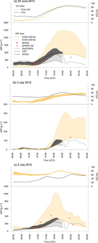
H. Rybka et al.: Modeling summer convection with ICON-LEM                                                                     4287

(Cioni and Hohenegger, 2017). ICON has also been used at            sensitivity experiments are important for understanding the
a lower storm-resolving resolution to study the spatial statis-     uncertainty connected with convectively generated precipi-
tics of deep tropical convection (Senf et al., 2018). In this       tation and climate-relevant aspects such as the longer-term
paper we use the unique capabilities of the HD(CP)2 system          impact of convection on the upper-tropospheric water bud-
to simulate realistic summer convective situations over land,       get.
where large amounts of convective available potential energy           To investigate the uncertainty of convection in high-CAPE
(CAPE) build up during the course of the diurnal cycle, as a        weather situations, we first select several summer convec-
tool to study the evolution of a convective system and the          tive events over Germany that feature (i) strong and deep
skill of the model simulating that system as well as to inves-      convective cells with little advection (e.g., 4 July 2015
tigate the uncertainty of forecasting such events.                  extending into 5 July 2015), (ii) large convective cells
   The difficulty of predicting precipitation location and          connected with frontal passages (e.g., 20 June 2013 and
amount arises to a large degree from the nonlinearity orig-         5 July 2015), and (iii) small-scale scattered convective sys-
inating from convective instability. Underlining that, Keil         tems (e.g., 3 June 2016), which are then simulated at 150 m
et al. (2014) established that predictability of convective pre-    resolution. See Table 1 for a list of all considered days.
cipitation depends on the convective adjustment timescale,             To evaluate the performance of the control and sensitiv-
with higher predictability during strong large-scale forc-          ity simulations of summer continental convection, we use
ing. Further, using a convection-permitting model covering a        ground-based and satellite observations from polar-orbiting
large domain, Selz and Craig (2015) demonstrated that initial       and geostationary sensors. To assess the quality of the high-
error growth is largest where the precipitation rate is large.      resolution simulations we rely on a suite of satellite ice water
Initial error growth in the first hour transitions to large-scale   path (IWP) products representing the range of uncertainty in
perturbations on a 12 h timescale. Moreover, resolutions of         state-of-the-art retrievals. Furthermore, cloud ice water con-
O(100 m) are necessary to realistically resolve and reproduce       tent (IWC), cloud-top height (CTH), and an instrument-like
deep moist convection (Bryan et al., 2003).                         ice cloud cover (ICC) conclude the evaluation of deep con-
   Given the difficulties in predicting the triggering of con-      vective clouds.
vection under widespread CAPE and moderate westerly ad-                The challenge of providing a meaningful comparison of
vection, sensitivities to the large-scale forcing and micro-        cloud-ice-related quantities with spaceborne observations
physics, as key players in the physics of moist convection,         was reported in Waliser et al. (2009). Several follow-up stud-
are explored. We aim to evaluate ICON-LEM simulations               ies (Eliasson et al., 2011; Waliser et al., 2011; Stein et al.,
regarding the water input into the upper troposphere due to         2011; Li et al., 2012; Eliasson et al., 2013; Li et al., 2016;
summertime moist convection and the temporal evolution of           Duncan and Eriksson, 2018) discussed the importance of
the resulting anvil cloud. We employ a number of remote             considering the uncertainties in satellite IWP observations
sensing products to explore whether our simulations of moist        and their limitations for model evaluation. In order to ana-
deep convection and their impact on the ice cloud field can be      lyze simulated cloud ice, it is necessary to know the unavoid-
constrained by observations. Given the verification against a       able constraints of satellite observations. These range from
collection of observational data sets, we aim to arrive at a        retrieval sensitivities to microphysical assumptions (Yang
tool to investigate the uncertainty of convection. The differ-      et al., 2013), spatial and temporal sampling characteristics
ent wavelengths used for observational estimates results in a       (Eliasson et al., 2013), and ultimately limitations that are de-
spread that can be compared with forecast uncertainty from          termined by instrument type (active or passive sensors). This
ICON-LEM sensitivity experiments.                                   study uses a suite of observational data sets that reflects a
   To that effect, we use boundary and initial conditions from      realistic range of retrieval uncertainties for constraining the
three operational NWP systems: the COnsortium for Small-            simulated cloud ice. These data sets encompass passive op-
scale MOdeling (COSMO) at 2.8 km, ICON at 13 km, and                tical observations with high temporal resolution by the Me-
the Integrated Forecast System (IFS) at 16 km. Because the          teosat Second Generation (MSG) satellite and with high spa-
boundary and initial conditions are from short forecasts close      tial resolution by polar-orbiting platforms. To explicitly show
to the analysis time, one might expect little impact on the         uncertainties of satellite ice products, different retrieval re-
ICON-LEM simulations. Additionally, we use the sensitivi-           sults are shown. In addition, a passive microwave sensor is
ties to the choices within the cloud microphysics parameteri-       also considered to complement the optical instruments.
zation, such as ice particle shape, to explore the sensitivity to      The structure of the paper is as follows. Section 2 gives a
model error. In the literature one can find numerous studies of     synoptic overview of the selected cases to describe the mete-
the sensitivity of convective storms and tropical cyclones to       orological background of the convective events. We describe
cloud microphysics (Wang, 2002; Milbrandt and Yau, 2006;            the model simulations and the observations used for verifi-
Li et al., 2009; Van Weverberg et al., 2012; Bryan and Mor-         cation in Sects. 3 and 4. The evaluation of the ICON-LEM
rison, 2012, among many others). Most of them report sig-           against observations is detailed in Sect. 5, while Sect. 6 de-
nificant sensitivity, especially through the impact of evapo-       scribes the sensitivity studies for varying boundary and ini-
ration and melting on the strength of the cold pool. Those

https://doi.org/10.5194/acp-21-4285-2021                                             Atmos. Chem. Phys., 21, 4285–4318, 2021
4288 H. Rybka et al.: Modeling summer convection with ICON-LEM
Table 1. Description of simulated convective days. Focus days ana- vection developed all day along a convergence zone, pre-
lyzed in more detail in Sects. 2, 5.2, and 6 are marked in bold font. dominantly in the western and northern part of Germany,
favored by hot surface temperatures above 35 ◦ C under un-
Simulation date Type of convection stable atmospheric conditions. Radiosonde data from Lin-
20 June 2013 highly organized frontal convection denberg (Fig. 2a) point at high CAPE values and signif-
29 July 2014 scattered deep convection icant convective inhibition (CIN) over the east of the do-
4 July 2015 large-scale convective clusters main, with a strong tropopause inversion at 190 hPa. Heavy
5 July 2015 convection embedded in front rainfall including large hailstones above 5 cm was reported
29 May 2016 strong convective phase with heavy rain for this day (https://eswd.eu/cgi-bin/eswd.cgi, last access:
and severe flooding in southern Germany 20 October 2020; Dotzek et al., 2009). Comparing the real
3 June 2016 scattered convection and synthetic satellite images for 20 June 2013 in Fig. 1
6 June 2016 distinct diurnal cycle of convection (top and middle rows in column a) shows similar cloud
22 June 2017 strong convective phase with heavy rain structures around noon. The simulated CAPE field reflects
huge potential for highly unstable regions (CAPE values over
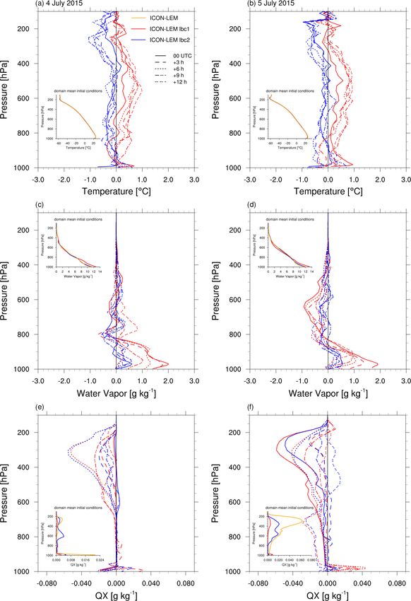
Table 2. Simulations with modified initial and lateral boundary con- 3000 J kg−1 ) above Germany. Based upon this single metric
ditions. it can be seen that once convective inhibition is overcome,
the potential to produce strong updrafts is given almost ev-
Simulation name Analysis Original Frequency erywhere.
resolution of analysis Furthermore, a 48 h period starting at 00:00 UTC on
ICON-LEM (default) COSMO-DE 2.8 km 3h 4 July 2015 has been chosen, which witnessed multiple lo-
ICON-LEM lbc1 ICON-NWP 13 km 12 h∗ cal explosive convection cells on the first day and convection
ICON-LEM lbc2 IFS 16 km 12 h∗ connected with a more synoptic-scale frontogenesis on the
second day (columns b and c in Fig. 1). For both days tem-
∗ Between analysis time steps, forecasts were used as lateral boundary conditions.
peratures of nearly 40 ◦ C were registered, which support lo-
calized triggering of convection under unstable atmospheric
conditions. Both criteria (high surface temperatures and un-
tial conditions as well as model physics before we conclude
stable conditions in the lower and middle troposphere) were
in Sect. 7.
fulfilled on 4 July, leading to the formation of a couple of
convective cells over the northern part of Germany. The ra-
2 Synoptic overview diosonde data from Bergen (Fig. 2b), very close to a convec-
tive cell, show large CAPE values and close to no CIN, with a
Three summer days, 20 June 2013 and 4–5 July 2015, strong tropopause inversion at 170 hPa. The development of
have been chosen to represent different high-CAPE sum- these cells was quite explosive, resulting in a strong upward
mer convection types. In Fig. 1 snapshots of SEVIRI (Spin- transport of moisture. Despite the convective region being
ning Enhanced Visible and Infrared Imager) satellite images highly localized, upper-tropospheric detrainment of mois-
are juxtaposed with synthetic SEVIRI images for the re- ture and ice by deep convection created an extensive cirrus
spective days. The synthetic SEVIRI images were produced shield covering the entire northeastern part of Germany by
with RTTOV (Radiative Transfer for TOVS; Saunders et al., the evening (not shown). Although the comparison of the ob-
1999, 2018) using as input ICON-LEM profiles of temper- served and simulated cloud fields in Fig. 1b reveals structural
ature, specific humidity, cloud liquid water content (LWC), differences, the overall ability of the model to simulate con-
and cloud ice water content (IWC), as well as simulated sur- fined convective cells is clearly visible in the CAPE field.
face skin temperature and 10 m wind speed. The ice opti- Circular white areas of consumed CAPE are located in the
cal properties come from the Baran parameterization (Vidot northern part of Germany surrounded by regions of higher
et al., 2015), and trace gas profiles were set to the RTTOV CAPE.
reference profiles. The red–green–blue (RGB) composites The situation on 5 July is characterized in the morning by
use the 0.6 µm reflectance for the red channel, the 0.8 µm re- the decay of the large-scale convective system of the previ-
flectance for the green channel, and the average of the 0.6 ous day and later by a transition of a front aided by dynam-
and 0.8 µm reflectance for the blue channel. In addition, sim- ical lifting induced by an upper-air trough located over the
ulated CAPE values from ICON-LEM are displayed in the North Sea. The satellite image in Fig. 1c shows the passage of
lowermost row in Fig. 1 for the respective time slices indi- the frontal system. The model produces an excessively large
cating atmospheric unstable regions. cloud structure that also extends too far south. Regions indi-
The first selected day covers the evolution of a frontal zone cating very high CAPE are almost gone at 16:00 UTC, with
on 20 June 2013. Germany lay between the ridge of an anti- Bergen showing relatively low values of CAPE (Fig. 2c), but
cyclone spanning from the central Mediterranean Sea to the larger values above 1000 J kg−1 occur over the northeastern
Baltics and a low-pressure system in France. Organized con- part of Germany.
Atmos. Chem. Phys., 21, 4285–4318, 2021 https://doi.org/10.5194/acp-21-4285-2021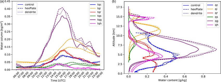
H. Rybka et al.: Modeling summer convection with ICON-LEM                                                                              4289

Figure 1. Synoptic situation as seen by SEVIRI for specific snapshots of the three selected days (upper row). Synthetic SEVIRI images of
simulated cloud fields created with RTTOV are shown in the middle row. The false-color satellite images, both real and simulated, use the
0.6 µm reflectance for the red band, the 0.8 µm reflectance for the green band, and the average of the red and green bands for the blue band.
Simulated CAPE values are displayed in the last row including the location of ground-based observational sites and initial release points
of radiosondes: Bergen (diamond), Lindenberg (circle), Jülich (triangle), and Leipzig (square). SEVIRI images show the area from 47.6 to
54.5◦ N and 4.5 to 14.5◦ W. Due to a change in the model domain for the 4 and 5 July simulations the western border is shifted by 1◦ .

   Each day presents a unique convective development, mak-               3   Model and simulations
ing these three cases an optimal test suite to study model per-
formance under unstable atmospheric conditions.                          Simulations have been performed using the ICON modeling
                                                                         framework developed by the German Meteorological Service
                                                                         and the Max Planck Institute for Meteorology (Zängl et al.,
                                                                         2015). Developments within HD(CP)2 led to an ICON ver-

https://doi.org/10.5194/acp-21-4285-2021                                                   Atmos. Chem. Phys., 21, 4285–4318, 2021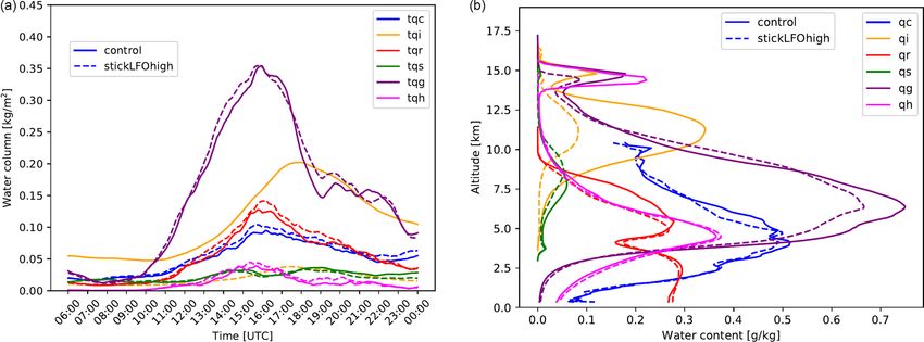
4290                                                        H. Rybka et al.: Modeling summer convection with ICON-LEM

sion specifically designed for regional to global large-eddy         In addition to the three days of interest described in Sect. 2,
simulations (Dipankar et al., 2015). Several high-resolution      we further analyze five additional high-CAPE summer con-
model runs covering Germany with a grid mesh of 625 m             vection days, including small-scale scattered convection (Ta-
have been carried out using realistic topography. Two addi-       ble 1). These cases are analyzed in a statistical manner to-
tional one-way nested domains with 312 and 156 m resolu-          gether with the three focus days in Sect. 5.3, which summa-
tion are also simultaneously embedded in the model runs us-       rizes the overall performance of ICON-LEM in representing
ing the lateral boundary conditions from the relative outer       atmospheric ice quantities in connection with deep convec-
ones. The coarsest-resolution (625 m) domain is referred to       tion.
as DOM01, whereas the one with the finest grid size (156 m)          Several sensitivity experiments have been conducted. The
is referred to as DOM03. Data from DOM02 (312 m horizon-          first set of additional simulations investigates the dependence
tal resolution) are not used in this paper. The vertical model    of model performance on the initial and lateral boundary con-
grid consists of 150 levels, with layer thickness gradually in-   ditions (lbc). Two additional analyses from ICON-NWP (us-
creasing from 20 m in the lowermost model layer to 380 m          ing the forecast system of DWD based on ICON) and IFS
at the top at 21 km in a height-based terrain-following co-       (cycle 41r1) models with lower spatial resolution (Table 2)
ordinate system (Leuenberger et al., 2010). Using a model         have been remapped onto the ICON-LEM grid in order to
of hectometer scale over a huge domain inherently leads to        initialize and force the high-resolution model during run-
resolved cloud dynamics; however, cloud microphysics, tur-        time. The temporal update of the lateral boundary forcing
bulence, and radiation still need to be parameterized.            is the same for all three cases. The only difference for IFS
   A complete summary of the model setup and the physics          and ICON-NWP forcing is that between analysis time steps,
package is given in Heinze et al. (2017) and references           3-hourly forecasts are available as boundary conditions (Ta-
therein. Here only the model aspects most relevant to this        ble 2). Using a different and/or coarser analysis allows us to
study are described. The following parameterizations have         address the sensitivity of ICON-LEM to large-scale forcing.
been used: a diagnostic Smagorinsky scheme with modifi-           Because ICON was made operational at DWD in 2015, this
cations by Lilly (1962) to account for subgrid-scale turbu-       analysis has only been performed for the 4–5 July 2015 case
lence and an all-or-nothing approach for cloud cover ne-          (Sect. 6.1).
glecting subgrid-scale cloud fractions. The microphysical            A second set of sensitivity experiments deals with changes
parameterization is based on Seifert and Beheng (2006a)           to the two-moment microphysics scheme of Seifert and Be-
and applies a two-moment mixed-phase bulk scheme (SB              heng (2006a, b) (Appendix A4; Table A1). The prognostic
scheme). Cloud condensation nuclei (CCN) concentration            variables within the SB scheme consist of the particle num-
is prescribed as a function of pressure and vertical ve-          ber concentration and mass mixing ratio of six different hy-
locity (Hande et al., 2016). The CCN concentration de-            drometeor categories, namely cloud water, rain, and four ice
creases above 1500 m and is almost constant below. It repre-      crystal classes: cloud ice, snow, graupel, and hail. The spe-
sents typical aerosol conditions simulated with the COSMO-        cific type or geometry of a frozen hydrometeor is referred to
MUSCAT model (Multi-Scale Chemistry Aerosol Transport;            in the following as a habit. We focus on the sensitivity sim-
Wolke et al., 2004, 2012). Ice nucleation is separated into a     ulations connected with ice crystal properties. In order to ac-
homogeneous and heterogeneous part. Homogeneous freez-            count for different ice crystal geometries and associated fall
ing follows the description of Kärcher and Lohmann (2002)         velocities based on Heymsfield and Kajikawa (1987), two
and Kärcher et al. (2006), whereas the quantity of heteroge-      separate simulations have been performed to specify cloud
neously nucleated ice particles is based on mineral dust con-     ice as hexagonal plates (simulation: “hexPlate”) or dendrites
centrations as described in Hande et al. (2015). The Rapid        (simulation: “dendrite”), both of which have lower terminal
Radiative Transfer Model (Mlawer et al., 1997) is used for        fall velocities compared to the default setup. A further sen-
radiative transfer calculations.                                  sitivity experiment, named “stickLFOhigh”, explores the im-
   Model runs of 24 h starting at 00:00 UTC have been per-        pact of increased sticking efficiencies during ice hydrome-
formed to investigate the ability of a high-resolution cutting-   teor collisions (snow–snow, ice–ice, snow–ice, and graupel–
edge model to forecast convective systems, especially to re-      snow) using parameters from Lin et al. (1983). The modi-
produce atmospheric ice composition.                              fied coefficients for the different sensitivity experiments are
   The default ICON-LEM setup uses an initialization in-          shown in Table 3. These simulations have been performed on
terpolated from the 2.8 km COSMO-DE (Baldauf et al.,              the coarsest model grid of 625 m (DOM01). All microphys-
2011) analysis of the German operational numerical weather        ical sensitivity studies correspond to the 5 July 2015 case
model. Moreover, 3-hourly COSMO-DE analysis is used to            and are discussed in Sect. 6.2. Only for these microphysical
relax ICON-LEM at the lateral boundaries using a 20 km            sensitivity studies do we make use of an explicit coupling
nudging zone and COSMO-DE forecasts every hour be-                of the two-moment microphysics scheme with radiation by
tween. Unless stated otherwise, the DOM03 simulations used        calculating the effective radii of cloud ice and cloud droplets
this setup.                                                       based on the predicted mass and number densities as well as
                                                                  the assumed particle size distribution.

Atmos. Chem. Phys., 21, 4285–4318, 2021                                             https://doi.org/10.5194/acp-21-4285-2021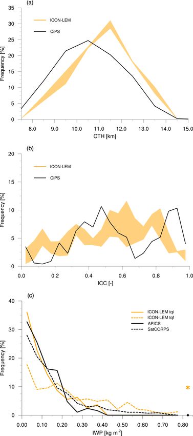
H. Rybka et al.: Modeling summer convection with ICON-LEM                                                                                     4291

Table 3. Power-law coefficients for the maximum diameter D and terminal fall velocity v of particles with mass m and parameters de-
termining the temperature-dependent (T ) sticking efficiency Estick (T ) of ice hydrometeor collisions used in the microphysical sensitivity
simulations.

                           Simulation name                         a             b                α           β    γ     ceff
                                                            (m kg−b )                  (m s−1 kg−β )
                           ICON-LEM (DOM01)                     0.835       0.390                  27.7   0.216   0.4    0.09
                           hexPlate                             0.220       0.302                  41.9   0.260   0.4    0.09
                           dendrite                             5.170       0.437                  11.0   0.210   0.4    0.09
                           stickLFOhigh                         0.835       0.390                  27.7   0.216   0.4   0.025

                         D(m) ∼ = amb.
                                             γ
                         v(m) =∼ αmβ ρ0 , with density ρ and surface density ρ0 = 1.225 kg m−3 .
                                         ρ
                         Estick (T ) = exp(ceff (T − T3 )), with freezing temperature T3 = 273.15 K.

4    Observational methods and data sets                                                – SPARE-ICE (Synergistic Passive Atmospheric Re-
                                                                                          trieval Experiment-ICE; Holl et al., 2014).
We use ground-based and satellite-based observations to
evaluate our simulations. Several previous studies have stated                       Four of them provide ice cloud properties with 15 min tempo-
the differing magnitude and sampling characteristics of                              ral resolution from the 12-channel SEVIRI imager aboard the
satellite-observed IWP or IWC (Waliser et al., 2009; Elias-                          geostationary MSG satellites (Schmetz et al., 2002), while
son et al., 2011; Hong and Liu, 2015; Duncan and Eriksson,                           two of them are from polar-orbiting satellites (see the next
2018). In evaluating the vertical and temporal distribution                          subsections for details). The different methods and charac-
of simulated atmospheric ice in terms of IWP or IWC it is                            teristics of the observational data sets are described in the
crucial to use multiple observational data sets representing a                       following.
range of algorithms in order to estimate retrieval errors and
uncertainties. For that reason, model simulations are com-                           4.1    RAMSES
pared to eight different observational methods, each of which
                                                                                     RAMSES is the operational high-performance multiparam-
has its own advantages and limitations.
                                                                                     eter Raman lidar at the Lindenberg Meteorological Obser-
   For a vertically resolved point-to-point evaluation of the
                                                                                     vatory (Reichardt et al., 2012). It is equipped with a water
simulations at different sites, two ground-based observations
                                                                                     Raman spectrometer (Reichardt, 2014) that facilitates direct
have been taken into account:
                                                                                     measurements of cloud water content (CWC) on a routine
    – RAMSES (Raman lidar for atmospheric moisture sens-                             basis. It is thus well suited for cloud microphysical studies
      ing; Reichardt et al., 2012) and                                               or for evaluating cloud models or the cloud data products of
                                                                                     other instruments. However, such CWC measurements are
    – Cloudnet retrievals (Illingworth et al., 2007).                                only possible at night under favorable atmospheric condi-
                                                                                     tions and often only in the lower cloud ranges because the
For full-domain model evaluation, ice cloud properties from                          Raman return signals from clouds are extremely weak, which
six different satellite retrieval algorithms are considered:                         makes them particularly vulnerable to background light and
                                                                                     light extinction. For cirrus clouds it was possible to overcome
    – SEVIRI CiPS (Cirrus Properties from SEVIRI; Strand-
                                                                                     this limitation by developing a retrieval technique that allows
      gren et al., 2017a),
                                                                                     for the estimation of IWC under all measurement conditions
    – SEVIRI SatCORPS (The Satellite ClOud and Radiation                             (see Appendix A1 and Fig. A1 for more details). The new
      Property retrieval System; Minnis et al., 2008; Trepte                         method was applied in conjunction with the case study of
      et al., 2019),                                                                 4–5 July 2015 in Sect. 5.2.

    – SEVIRI APICS (Algorithm for the Physical Investiga-                            4.2    Cloudnet
      tion of Clouds with SEVIRI; Bugliaro et al., 2011),
                                                                                     The ground-based data set from Cloudnet provides synergis-
    – SEVIRI CPP (Cloud Physical Properties from SEVIRI;                             tic products from 35 GHz cloud radar, ceilometer, and multi-
      Roebeling et al., 2006),                                                       frequency microwave radiometer measurements. These prod-
                                                                                     ucts are derived for the observation sites Jülich, Leipzig, and
    – MODIS C6 (Moderate Resolution Imaging Spectrora-                               Lindenberg using the same retrieval package developed in
      diometer Collection 6 Cloud Products; Platnick et al.,                         Cloudnet (Illingworth et al., 2007). Measurements are per-
      2017), and                                                                     formed day and night, and data are provided with a tem-

https://doi.org/10.5194/acp-21-4285-2021                                                                  Atmos. Chem. Phys., 21, 4285–4318, 2021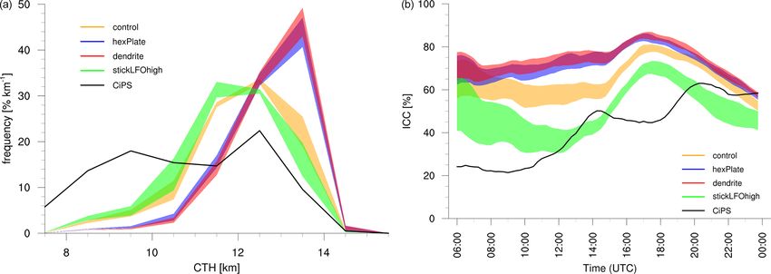
4292                                                           H. Rybka et al.: Modeling summer convection with ICON-LEM

poral and vertical resolution of 30 s and 60 m, respectively.        makes the algorithm unsuitable for the evaluation of mod-
Due to the low attenuation of the radar signals at this wave-        eled IWP in this paper, wherein thick convective clouds are
length in the cloudy atmosphere, clouds are detected in al-          analyzed, but CiPS is an ideal tool to study, e.g., the spatial
most their entire vertical extent depending on the radar sensi-      extent of anvil cirrus from the convective outflow including
tivity. Only in situations with strong precipitation is the atten-   the optically thinner cloud edges.
uation higher and thus the cloud detection capability lower.
   As the first step, the retrieval performs a target classifi-      4.4   SEVIRI APICS
cation including the determination of cloud base and top.
Radar profiles of reflectivity, Doppler velocity, and ceilome-       The Algorithm for the Physical Investigation of Clouds with
ter backscatter profiles are used for this purpose, as are tem-      SEVIRI (APICS; Bugliaro et al., 2011) computes optical
perature and humidity profiles provided by an NWP model              thickness τ and ice crystal effective radius reff for pixels
(e.g., COSMO-DE for Lindenberg) or radiosoundings. Verti-            identified as cirrus by CiPS by means of the Nakajima–
cal profiles of LWC and IWC are subsequently derived. For            King method (Nakajima and King, 1990) using two SEVIRI
echoes classified as ice, IWC is calculated from radar reflec-       solar channels centered at 0.6 and 1.6 µm. IWP is derived
tivity and temperature using an empirical formula, which was         from these two quantities (τ , reff ) under the assumption of
derived on the basis of a large midlatitude aircraft data set        a vertically homogeneous cloud layer using the relationship
(Hogan et al., 2006). The random error of the IWC retrieval          IWP = 2/3ρice reff τ , where ρice = 917 kg m−3 is the density
is approximately between +50 % and −33 % for IWC val-                of ice. The algorithm assumes the general ice crystal shape
ues in the range of 0.03 to 1 g m−3 . A potential systematic         mixture from Baum et al. (2011). Retrieved optical thickness
error in IWC, which is mainly caused by systematic errors in         is up to 200, while effective radius is between 5 and 60 µm,
radar reflectivity, is of the same order of magnitude assum-         yielding a maximum retrieved IWP of ≈ 7300 g m−2 . In con-
ing a radar calibration error of 2 dBZ. It should also be noted      trast to CiPS, APICS is not limited to thin cirrus but is only
that due to the limited sensitivity of the cloud radar, very thin    available during daytime.
clouds (with small ice crystals) may not be detected.
                                                                     4.5   SEVIRI SatCORPS
4.3    SEVIRI CiPS
                                                                     The Satellite ClOud and Radiation Property retrieval Sys-
The Cirrus Properties from SEVIRI (CiPS; Strandgren et al.,          tem (SatCORPS) is a comprehensive set of algorithms de-
2017a) algorithm detects cirrus clouds and retrieves their           signed to retrieve cloud microphysical and macrophysical in-
cloud-top height (CTH), ice optical thickness (τ ), and IWP          formation day and night from meteorological satellite im-
using thermal observations from MSG/SEVIRI. To this end,             ager data. These algorithms were originally developed for
a set of neural networks trained with SEVIRI observations            the NASA Clouds and Radiant Energy Systems (CERES)
and coincident cirrus properties retrieved with the Cloud-           project (Minnis et al., 2020; Trepte et al., 2019) and adapted
Aerosol LIdar with Orthogonal Polarization (CALIOP) in-              for application to other polar-orbiting and geostationary im-
strument (Winker et al., 2009) are used. Day and night cov-          agers, including SEVIRI. Using radiances in the 0.6 µm (vis-
erage, a temporal resolution of up to 5 min, and a spatial res-      ible), 3.9 µm (shortwave-infrared), 10.8 µm (infrared), and
olution of 3 km at nadir make the algorithm ideal for evaluat-       12.0 µm (split-window) bands, three different methods are
ing the temporal evolution of high cloud fields. CiPS targets        employed depending on time of day and cloud opacity to
thin cirrus clouds, detecting, compared to CALIOP, about             retrieve cloud optical thickness (τ ), ice crystal effective di-
50 %, 60 %, and 80 % of cirrus clouds with an ice optical            ameter (Deff = 2reff ), and cloud effective temperature (Tc ).
thickness of at least 0.05, 0.08, and 0.14 (Strandgren et al.,          During daytime, the visible-infrared shortwave-infrared
2017a), which corresponds to an IWP of roughly 0.6, 1.0,             split-window technique (VISST) uses the visible, shortwave-
and 3.0 g m−2 , respectively. The CTH retrieved by CiPS has          infrared, and infrared radiances to determine τ , Deff , and
an average error of 10 % or less for cirrus clouds with a            Tc , respectively, through an iterative process that also ex-
top height greater than 8 km, again with respect to CALIOP           ploits the split-window band to aid phase determination. The
observations over the entire MSG disk. When looking at               VISST is similar in essence to the classic Nakajima and King
the geographic distribution of CTH accuracy of CiPS ver-             (1990) bispectral method.
sus CALIOP, it turns out that the CiPS neural network has               For thin non-opaque cirrus (τ < 8) during nighttime, the
a mean percentage error very close to zero in Germany for            shortwave-infrared split-window technique (SIST) retrieves
ice clouds located between 8 and 11 km. For lower clouds,            the same parameters from brightness temperature differ-
CiPS tends to overestimate and for higher clouds to under-           ences between the shortwave-infrared and infrared bands
estimate CTH. The high sensitivity of CiPS to thin cirrus            and those between the infrared and split-window bands. The
does, however, lead to a quick saturation of the IWP and             VISST/SIST reflectance lookup tables (LUTs) and emittance
τ retrievals in thicker cirrus clouds. Maximum IWP and τ             parameterizations are calculated for smooth solid hexagonal
amount to approximately 100 g m−2 and 4, respectively. This          ice crystals. Assuming that the retrieved ice crystal effective

Atmos. Chem. Phys., 21, 4285–4318, 2021                                                https://doi.org/10.5194/acp-21-4285-2021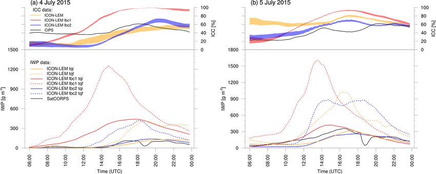
H. Rybka et al.: Modeling summer convection with ICON-LEM                                                                  4293

diameter represents the average over the entire cloud thick-       100 and 62.5 µm, respectively, which result in a maximum
ness, IWP is computed from the following cubic equation:           IWP of ≈ 3900 g m−2 . Due to the different assumed ice habit
                                                                   and smaller τ truncation threshold, SEVIRI CPP retrieves
                                    2
IWP = τ (0.259 Deff + 0.819 × 10⁻³ Deff                            smaller IWP values than SEVIRI APICS, although the al-
                                     3
                     − 0.880 × 10⁻⁶ Deff ).                 (1)    gorithms are otherwise very similar. Older versions of CPP
                                                                   and APICS are also shown in Bugliaro et al. (2011) to pro-
For thick opaque ice clouds (τ > 8) during nighttime, the Ice      vide similar results, with CPP again producing lower values
Cloud Optical Depth from Infrared using a Neural network           of optical thickness and IWP than APICS.
(ICODIN) method is used (Minnis et al., 2016), complement-
ing the SIST applicable to semitransparent cirrus. ICODIN          4.7   MODIS
retrieves τ and IWP by training shortwave-infrared, infrared,
and split-window radiances against the CloudSat radar-only         MODIS is a 36-channel imager with a spatial resolution of
2B-CWC-RO product (Austin et al., 2009), which includes            250, 500, or 1000 m at nadir and with a swath width of
vertical profiles of IWC and ice particle effective radius. The    2330 km. It is the key instrument aboard the Terra and Aqua
method can be used to derive ice cloud τ up to 150; how-           NASA satellites and provides global coverage every 1 or
ever, τ and thus IWP for the deepest convective clouds are         2 d. The MODIS cloud microphysical products are also ob-
still frequently underestimated. According to Eq. (1), with        tained by the Nakajima and King (1990) bispectral method
a maximum τ of 150 and a maximum effective diameter of             and provide daytime estimates of cloud optical thickness and
150 µm, the maximum IWP that can be derived using this ap-         ice particle effective radius from solar reflectances measured
proach is ≈ 8100 g m−2 . SatCORPS is the only geostation-          in a non-absorbing visible band and a water-absorbing near-
ary retrieval used here that provides IWP during both day          infrared band (Platnick et al., 2017). Three different spec-
and night for thin and thick ice clouds. Note, however, that       tral cloud retrievals are performed by combining the 0.66 µm
at the day–night transition, the weak solar component in the       channel separately with the 1.6, 2.1, and 3.7 µm channel, al-
3.9 µm band increases the uncertainty in the opaque vs. semi-      though here we only use the primary 0.66–2.1 µm channel
transparent cloud classification and can result in the use of      pair. In the latest Collection 6 algorithm, the plane-parallel
default values for τ (16 or 32), which are significant un-         reflectance LUTs are calculated for a single ice shape of
derestimates in deep convective clouds (see the sudden dip         severely roughened compact aggregates composed of eight
in IWP around 18:00 UTC in Fig. 5). Nighttime retrievals           solid columns. Assuming a vertically homogeneous cloud,
are inherently more uncertain due to the reduced information       the IWP is derived as for SEVIRI APICS and SEVIRI CPP.
content resulting from the lack of the solar reflectance chan-     The 1 km resolution IWP retrievals are available twice a day
nel (Minnis et al., 2020), and the nighttime algorithm has a       from the Terra and Aqua satellites, which are in a 10:30 local
tendency to favor ice-phase retrievals (Yost et al., 2020). The    solar time (LST) descending node and 13:30 LST ascending
pixel-level SEVIRI SatCORPS data at 15 min temporal reso-          node sun-synchronous polar orbit, respectively. Maximum
lution were obtained from the NASA Langley Research Cen-           retrieved optical thickness and effective radius are 100 and
ter (http://satcorps.larc.nasa.gov, last access: 15 April 2019).   60 µm, yielding a maximum retrieved IWP of ≈ 3700 g m−2 .
                                                                   Benas et al. (2017) compared SEVIRI CPP and MODIS re-
4.6   SEVIRI CPP                                                   trievals. They found lower CPP IWPs than MODIS IWPs,
                                                                   similar to our observations (see Fig. 5), mainly caused by
The Cloud Physical Properties (CPP) algorithm (Roebeling           lower CPP ice effective radius values.
et al., 2006) is a bispectral method (Nakajima and King,
1990), which uses SEVIRI 0.6 and 1.6 µm solar reflectance          4.8   SPARE-ICE
measurements to retrieve cloud optical thickness and ice
particle effective radius during daytime. The retrievals are       The Synergistic Passive Atmospheric Retrieval Experiment-
based on LUTs of top-of-atmosphere reflectances calculated         ICE (SPARE-ICE) features a pair of artificial neural net-
for plane-parallel layers of randomly oriented monodisperse        works that use infrared and microwave radiances as input to
roughened hexagonal ice crystals (Hess et al., 1998). Assum-       detect ice clouds and retrieve their IWP (Holl et al., 2014).
ing no vertical variation in ice crystal size, the IWP is calcu-   The networks were trained by collocating AVHRR chan-
lated as for APICS, although the density of ice is assumed         nel 3B, 4, and 5 (3.7, 10.8, 12 µm) and MHS channel 3,
to be ρice = 930 kg m−3 . Specifically, we use data from the       4, and 5 (183 ± 1, 183 ± 3, 190 GHz) radiances with IWP
CLoud property dAtAset using SEVIRI – edition 2 (CLAAS-            retrievals from the CloudSat/CALIPSO radar–lidar synergy
2) archive provided by the EUMETSAT Satellite Applica-             product 2C-ICE (Deng et al., 2010). The exclusion of solar
tion Facility on Climate Monitoring (Benas et al., 2017). The      reflectances from SPARE-ICE allows retrievals both day and
pixel-level IWP retrievals are available every 15 min at a spa-    night; however, the reliance on microwave measurements re-
tial resolution of ≈ 6 km over Germany. For this algorithm,        sults in fairly large footprints varying from 16 km in diame-
maximum retrieved optical thickness and effective radius are       ter at nadir to 52 × 27 km2 in areas at the edge of the scan.

https://doi.org/10.5194/acp-21-4285-2021                                           Atmos. Chem. Phys., 21, 4285–4318, 2021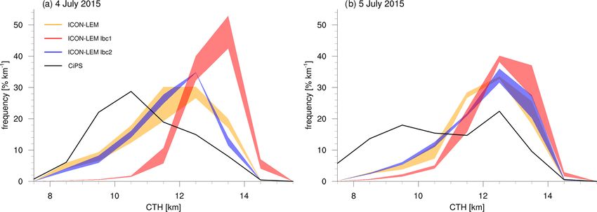
4294                                                           H. Rybka et al.: Modeling summer convection with ICON-LEM

The lower and upper sensitivity limits of SPARE-ICE are              used. In addition, the retrieved optical thickness and particle
10 g m−2 and O(104 ) g m−2 , respectively, with the median           effective radius strongly depend on the assumed ice parti-
fractional error between SPARE-ICE and 2C-ICE IWP being              cle shape (smooth or roughened, solid or hollow, hexagonal
a factor of 2. For the current study, data are available from the    columns or aggregates etc.), even for unsaturated input re-
MetOp-A/B (09:30 LST descending node) and NOAA-18/19                 flectances. For instance, Eichler et al. (2009) show that for
(15:00–16:30 and 13:30–14:00 LST ascending node) satellite           thin ice clouds with an optical thickness between 3 and 5,
overpasses.                                                          the choice of ice particle shape leads to uncertainties of up to
                                                                     70 % for optical thickness and 20 % for effective radius. Re-
4.9    Interpretation of satellite IWP retrievals                    trievals in deep convective clouds have uncertainties of a sim-
                                                                     ilar magnitude or even larger. As a last source of uncertainty
Despite the wide variety of available satellite instruments          one has to mention that passive optical retrievals assume the
(imagers, sounders, lidar, radar) and retrieval methods ex-          cloud to consist of either ice or liquid water clouds accord-
ploiting the information obtained with these instruments, de-        ing to their cloud-top phase. When both phases are present
termining atmospheric ice mass has been recognized as a              in convective clouds – liquid water in the lower and ice in
great challenge for remote sensing (Waliser et al., 2009;            the upper part, with a mixed-phase layer in between – the re-
Eliasson et al., 2011), which has seen only limited progress in      trieved IWP accounts in part for the liquid water layers and
the past decade as large discrepancies in IWP remain among           thus tends to overestimate the real IWP. However, the trunca-
satellite data sets (Duncan and Eriksson, 2018). In this con-        tion of the retrieved optical thickness mentioned above par-
text, “ice” represents all frozen hydrometeors, including the        tially compensates for this overestimation. Nevertheless, the
smaller suspended (or floating) cloud ice and the larger pre-        combination of all the above effects can easily lead to a fac-
cipitating forms such as snow, graupel, and hail. Current            tor of 2–3 variation in the estimated domain-mean IWP. In
satellite retrieval methods are unable to truly distinguish sus-     our Vis–NIR satellite data, SEVIRI CPP shows the smallest
pended ice from precipitating ice, which makes estimates             IWPs and SEVIRI SatCORPS the largest ones, with SEVIRI
from these techniques rather uncertain in thick, multilayer,         APICS and MODIS values being in between (see Fig. 5),
mixed-phase, and mixed-habit cloud fields. The measured              providing a broad range of estimates reflecting the current
signal, and hence the derived ice mass, is a weighted sum            state of the art.
of the individual contributions from the different ice habits.          The SPARE-ICE retrievals, on the other hand, were trained
Habit weighting, however, varies by retrieval method and             on CloudSat/CALIPSO active radar–lidar retrievals, whose
is poorly characterized if at all, which complicates model–          sensitivity is markedly shifted to the larger ice hydrometeors.
satellite comparisons because the various satellite products         Therefore, SPARE-ICE usually provides the highest IWPs
all refer to “ice water path”, without any qualifying caveats        due to the inclusion of graupel and hail, although the Sat-
about their differing sensitivities. In turn, this also means that   CORPS passive Vis–NIR retrieval can occasionally produce
different instruments are sensitive to different ice cloud types     IWPs of comparably large magnitude, as shown later.
(Eliasson et al., 2011) such that several spaceborne sensors            As a last issue, the different spatial resolutions of the satel-
are needed to cover the full range of ice clouds.                    lite measurements must be mentioned. Since MODIS pro-
   Passive visible–near-infrared (Vis–NIR) methods can de-           vides the finest resolution, SEVIRI an intermediate resolu-
rive IWP only indirectly from optical thickness and effective        tion, and SPARE-ICE the coarsest, MODIS is able to catch
particle size. However, they infer particle size from cloud-top      peaks of high IWP that are smoothed out in the other two
measurements and usually provide an estimate of cloud-top            observational data sets. However, the differences in instan-
ice particle size. Thus, they are unable to obtain information       taneous pixel-level estimates due to different spatial resolu-
about ice particle sizes in lower layers inside vertically thick     tions are largely reduced in domain-mean IWP.
clouds, and the bulk IWP formulas used that assume verti-               In our model validation effort, we follow a somewhat qual-
cal homogeneity (see Sect. 4.4, 4.6, and 4.7) cannot a priori        itative rule of thumb recommended by Waliser et al. (2009)
account for vertical variations in extended clouds.                  and consider the SEVIRI/MODIS passive Vis–NIR IWP re-
   Furthermore, these methods are subject to saturation ef-          trievals to be more representative of the smaller suspended
fects (normally affecting a few percent of pixels in our ana-        cloud ice mass and treat the SPARE-ICE radar- and lidar-
lyzed scenes, mainly the convective cores; in situations with        trained IWP retrievals as more indicative of the total ice mass
large-scale convective activity many pixels may be affected,         (i.e., cloud plus precipitating ice).
e.g., 20 % of pixels on 20 June 2013) because visible re-
flectance loses sensitivity to optical thickness in thick clouds.    4.10   Comparison to model simulations
As a result, the maximum reported optical thickness is trun-
cated at a threshold value varying between 100 and 200 de-           When comparing vertical profiles of cloud hydrometeors
pending on the data product. The maximum reported ice par-           from ICON-LEM to surface lidar (RAMSES, Sect. 4.1) or
ticle effective radius also varies among data sets, although         radar (Cloudnet, Sect. 4.2) observations, the model grid
in a narrower range, depending on the ice optical properties         points nearest the locations of ground-based instruments are

Atmos. Chem. Phys., 21, 4285–4318, 2021                                                https://doi.org/10.5194/acp-21-4285-2021
H. Rybka et al.: Modeling summer convection with ICON-LEM 4295
selected. Furthermore, we take into account the neighbor- resolution version of ICON in simulations over the equato-
ing grid points since differences between observations and rial Atlantic (Senf et al., 2019). More specifically, the impact
simulations may be easily explained in the case of inhomo- of deep summertime convection on ice cloud properties is
geneities. This comparison approach is intended to provide investigated over Germany. We focus on a few case studies
an assessment of the model simulation error considering po- (Sect. 2) and study the evolution of the convective outflow
tential temporal or spatial displacements. by making use of radiosonde data, remote sensing data from
When comparing model quantities with satellite observa- ground-based instruments, and instruments on geostationary
tions, we proceed as follows. Ice cloud cover (ICC) and CTH and polar-orbiting satellites (Sect. 4).
are evaluated against CiPS retrievals (Sect. 4.3), which have
a high detection efficiency for ice clouds, including thin ice 5.1 Evaluation of simulated temperature profiles with
clouds. In order to compare the CiPS results with modeled radiosonde data
ICC and CTH, we need to consider the detection efficiency
dependent on IWP or optical thickness of CiPS. We there- This section is dedicated to presenting a comparison of sim-
fore calculate IWP from the simulated cloud fields and re- ulated thermodynamic profiles and radiosonde data for spe-
spectively apply cutoff values of 0.6 and 3.0 g m−2 , corre- cific locations and times for each summertime convective
sponding to the 50 % and 80 % detection probability of CiPS event presented in Sect. 2. The comparison with model data
(see Sect. 4.3). The resulting IWP is called IWPCiPS−sim provides a brief verification of the model setup and its ability
in the following. IWPCiPS−sim of the simulated cloud field to reproduce the stability and moisture profile as well as how
is calculated from IWC and LWC below −25 ◦ C because conducive it is for deep convection including an indication
CiPS increasingly misidentifies supercooled liquid water as of possible cloud-top height. For this evaluation of temper-
ice at lower temperatures (Strandgren et al., 2017b). Above ature profiles, observational radiosonde data archived at the
−25 ◦ C it is calculated from IWC only if IWC is larger than Climate Data Center of the German Weather Service (https:
LWC. If IWPCiPS−sim does not exceed the threshold value, //opendata.dwd.de/climate_environment/CDC/, last access:
cloud cover is set to 0.0. CTH in turn is set to the height at 13 November 2020) have been used.
which IWPCiPS−sim first exceeds the threshold when integrat- Figure 2 shows three different atmospheric profiles mea-
ing IWPCiPS−sim from the top of the cloud layer. The ICC and sured by radiosonde soundings presented in Skew-T and log-
CTH calculated for the two IWP thresholds give a measure of P diagrams. The location and time of ascent are stated above
the uncertainty in the CiPS retrievals. Very thin simulated ice each panel and closely match the snapshots in Fig. 1. When
clouds (IWP < 0.6 g m−2 ) are neglected, and the influence of comparing the model simulation with the radiosonde mea-
mixed-phase clouds is limited in our analyzed ICC and CTH. surements the drift of the radiosonde during the ascent has
We note that the above CiPS-specific ICC should not be con- been taken into consideration to adjust the location, time, and
fused with the model’s own output variables of high cloud pressure altitude of the simulated profile in accordance with
cover or cirrus cloud cover, which are calculated differently. the drift. The red lines illustrate an undiluted air parcel as-
IWP averaged over the whole simulation domain is com- cent above the level of free convection and visualize the cor-
pared to the satellite products from Sect. 4 to account for responding CAPE. CAPE values are given above each figure.
the uncertainty in IWP retrievals. The SatCORPS retrieval Figure 2a shows measured (black) and simulated (blue)
method switches input channels at sunset between 18:00 and profiles at Lindenberg for 20 June 2013 at 12:00 UTC. The
19:00 UTC (see Sect. 4.5), which leads to unreliable esti- comparison illustrates very similar temperature (solid lines)
mates around that time. Furthermore, two separate domain- and dew-point temperature (dashed lines) profiles, reflect-
averaged IWP values are calculated from ICON-LEM data: ing a high-CAPE (red) environment. CIN is higher in the
one strictly for cloud ice water path (tqi) and one for total simulation than in observations, which is dominated in both
frozen water path (tqf). The former is the column-integrated observations and simulations by an inversion layer of sev-
and domain-averaged ice content (qi) of cloud ice crystals eral Kelvin. A tropopause inversion is seen in the measured
only, whereas tqf comprises all ice habits, including the profiles, which is less sharply reproduced by ICON-LEM,
larger agglomerates such as snow (qs), graupel (qg), and hail highlighting possibly higher cloud tops than observed. In the
(qh) within the two-moment microphysics. Please refer to simulation, the upper troposphere at around 200 hPa is ice-
Sect. 4.9 for a discussion about the sensitivity of the single saturated, while observations indicate slightly lower relative
satellite retrievals to different ice classes. humidity.
Explosive localized convective cells characterize the day
of 4 July 2015. One of these cells was located in the vicin-
5 Evaluation of ICON-LEM simulations against ity of Bergen, which happened to serve as a launching po-
observations sition for a radiosonde ascent. The corresponding profile is
shown in Fig. 2b. The simulated dew-point (blue dashed) and
We focus on ice cloud properties in the ICON-LEM simula- temperature (blue solid line) profile closely follow the ob-
tions, which have until now only been evaluated in a lower- served ascent up to 500 hPa, reproducing the very dry layer
https://doi.org/10.5194/acp-21-4285-2021 Atmos. Chem. Phys., 21, 4285–4318, 2021You can also read