Munich, 12-13 October 2020 Wages, Rents, and the Quality of Life in the Stationary Spatial Equilibrium with Migration Costs - Gabriel M. Ahlfeldt ...
←
→
Page content transcription
If your browser does not render page correctly, please read the page content below

Munich, 12–13 October 2020

Wages, Rents, and the Quality of Life in the
Stationary Spatial Equilibrium with Migration
Costs
Gabriel M. Ahlfeldt, Fabian Bald, Duncan Roth, and Tobias Seidel
Wages, rents, and the quality of life in the stationary spatial
                          equilibrium with migration costs∗

                               †                        ‡                         §                        ¶
    Gabriel M. Ahlfeldt                Fabian Bald             Duncan Roth               Tobias Seidel

                                             October 2, 2020

                                                Abstract
   We develop a dynamic spatial model in which workers belonging to an arbitrary number of
   groups choose among an arbitrary number of local labour markets facing costs and returns
   to agglomeration. The model features imperfect spatial arbitrage and does not impose
   any restriction on the spatial distribution of worker utility. Heterogeneous workers are
   imperfectly mobile and forward-looking and yet all structural fundamentals can be inverted
   without assuming that the economy is in a spatial steady state. Exploiting these novel
   features of the model, we show that the canonical spatial equilibrium framework understates
   spatial quality-of-life differentials, the urban quality-of-life premium and the value of local
   non-marketed goods. We also show how to use the model to quantitatively evaluate the
   welfare effects of place-based policies in account of the efficiency-equity trade-off that shapes
   spatial policies.
   Key words: Migration, dynamic, wages, rents, spatial equilibrium, quality of life, welfare
   JEL: R38, R52, R58

    ∗
      Due to confidentiality requirements, we use a restricted version of the IAB data set at some stages of the
model quantification. This may result in small changes in our quantitative results in the final version. We
thank seminar, conference, and workshop participants in Amsterdam (Tinbergen), Duisburg-Essen (Uni),
EALE (online), EEA (online), Essen (RWI), Ispra (EC Joint Research Center, online), London (LSE),
Lyon (GATE), Paris (HEC, virtual), Potsdam (VfS), Rome (BOI), and St. Gallen (Uni) for comments and
suggestions, in particular Michael Amior, Thomas Bauer, Kirill Borusyak, Helge Braun, Martin Brown,
Gilles Duranton, Christian Dustmann, Roland Fuess, Cecile Gaubert, Christoph Hank, Vernon Henderson,
Christian Hilber, Philip Jung, Hans Koster, Joan Monras, Guy Morrell, Jos van Ommeren, Florian Oswald,
Fernando Parro, Jacques Poot, Esteban Rossi-Hansberg, Olmo Silva, Daniel Sturm and Coen Teulings for
comments and suggestions. The usual disclaimer applies.
    †
      London School of Economics, CEPR & CESifo
    ‡
      Universität Duisburg-Essen, RGS
    §
      Institut für Arbeitsmarkt- und Berufsforschung (IAB), Nürnberg
    ¶
      Universität Duisburg-Essen, CESifo & CRED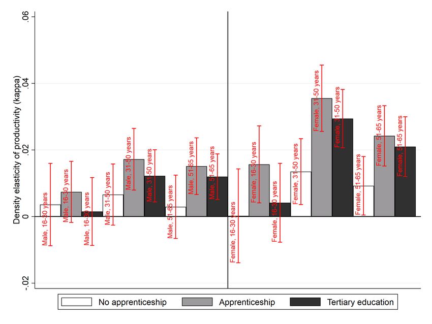
A     Introduction
In economics, quality of life (QoL) is a location-specific utility shifter that can be used
to value local public goods or bads such as clean or dirty air. From Ricardo (1817)
via the neoclassical Rosen (1979)-Roback (1982) framework to quantitative spatial models
(QSMs) summarized by Redding and Rossi-Hansberg (2017), economists have inferred QoL
assuming a competitive spatial equilibrium (CSE) in which free mobility of homogeneous
workers leads to perfect spatial arbitrage. Spatially invariant utility then ensures that
spatial differences in amenity values are offset by differences in real wages, the so-called
compensating differential. In reality, workers rarely move between labour market areas
more than once or twice over their employment biography, owing to idiosyncratic tastes
for locations and non-pecuniary migration costs that typically exceed the equivalent of an
annual income (Koşar et al., 2019). Hence, spatial arbitrage is likely imperfect, raising a
range of important questions. How should we measure QoL without imposing an exogenous
reservation utility level? How should we value local non-marketed goods if real wage
differences do not map directly to compensating differentials? How should we evaluate
the aggregate and distributional consequences of QoL policies in a frictional world with
spatial incidence, i.e. persistent localized utility effects?
    To answer these questions, we develop a quantitative general equilibrium model that
combines the strengths of two recent classes of spatial models. It inherits the complete
invertibility from QSMs (Allen and Arkolakis, 2014; Ahlfeldt et al., 2015; Monte et al.,
2018) and the ability to account for frictional adjustments in the spatial economy from
dynamic spatial models (DSMs) (Desmet et al., 2018; Caliendo et al., 2019a; Monras,
2020). Specifically, we propose the first DSM with heterogeneous, imperfectly mobile
and forward-looking agents that can be fully quantified without imposing the unrealistic
assumption that the economy is in a spatial steady state. We exploit this novel feature for
a threefold contribution. First, we propose a new approach to measuring QoL that allows
for worker heterogeneity and costly migration and does not impose any restriction on the
spatial distribution of worker utility. Second, we show theoretically and empirically that
the canonical CSE framework severely understates spatial differentials in QoL, the urban
QoL premium, and the value of local public goods. Third, we illustrate how the welfare
effect of spatially targeted QoL policies critically depends on the social welfare function,
owing to imperfect spatial arbitrage, displacement effects, and spatial incidence.
    Our quantitative model incorporates an arbitrary number of worker groups and an
arbitrary number of local labour markets that are interconnected through costly migra-
tion. Following the conventions in the literature, we treat QoL as a group-region-specific
structural fundamental that shifts utility. Locations further differ in terms of exogenous
housing productivity and land supply. Labour productivity is group-region-specific and
consists of an exogenous component and an endogenous component that positively de-
pends on density (Combes and Gobillon, 2015). Labour is the only factor of production
used to produce one final good which is freely traded and consumed at a spatially invariant

                                                1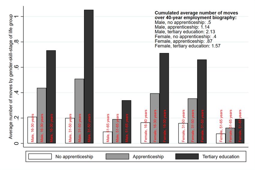
price. Housing is produced by developers who use capital and land from absentee owners
as inputs. Workers spend their labour income on the tradable good and housing. All
markets are competitive. Inelastic supply of land generates a dispersion force in the form
of high rents in places in high demand (Combes et al., 2019).
   Unlike in CSE models that assume perfect spatial arbitrage, spatial arbitrage is an
endogenous mechanism in our model that operates through migration. Intuitively, mi-
gration into an attractive region congests the housing market, leading to subsequently
reduced in-migration as long as the housing-market-related congestion force exceeds the
labour-market-related agglomeration force. Concretely, we model migration as an invest-
ment decision in which workers choose destinations facing a trade-off between the present
value of expected utility flows and a one-off relocation cost. Following the discrete choice
literature in the tradition of McFadden (1974), workers receive bilateral amenity shocks
with an idiosyncratic and a group-year-specific component. This stochastic formulation
provides the microeconomic foundations for a migration gravity equation that has been
found to be empirically successful (Kennan and Walker, 2011; Bryan and Morten, 2019;
Tombe and Zhu, 2019). The dispersion of the idiosyncratic shocks is inversely related
to the migration elasticity, which monitors how strongly bilateral migration probabilities
respond to differences in expected indirect utility at migration destinations. If the migra-
tion elasticity approaches zero, shocks to labour and housing productivity or QoL will not
trigger migration so that any localized utility effect remains persistent. If the migration
elasticity approaches infinity, there is no taste heterogeneity so that migration will go on
until a shock that has caused migration is fully offset by adjustments in wages and rents.
Spatial arbitrage is then perfect. We show that for values of the migration elasticity found
in our data and in previous research (Caliendo et al., 2019b), the marginal worker’s will-
ingness to accept high real living cost steeply decreases in the size of a local labour market.
Therefore, our model rationalizes real living cost differentials by much larger differences in
group-specific average QoL than the canonical CSE framework, leading to a higher urban
QoL premium and larger valuations of local public goods.
   When switching between labour markets, workers pay an origin-destination-group-
specific migration cost in the form of foregone utility in the relocation period. Workers
remaining at their origin incur no migration cost. Larger bilateral migration costs map to
smaller migration flows between local labour markets, leading to a lower speed of spatial
arbitrage. More generally, positive migration costs imply that spatial adjustments are
non-instantaneous, giving rise to the dynamic structure of the model and distinct notions
of spatial equilibria. In the absence of a consensus, we take the liberty of naming a tran-
sitory spatial equilibrium (TSE) and a stationary spatial equilibrium (SSE) that prevail in
the nascent DSM literature. The role of the TSE is to rationalize observed data assuming
that goods and factor markets clear without imposing any restriction on trends in prices
and quantities on labour and housing markets. In the SSE, goods and factor markets clear
and all prices and quantities are stationary. Intuitively, the SSE is a counterfactual situa-
tion to which a spatial economy would mean-revert in the absence of shocks to the labour

                                              2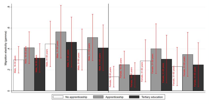
productivity, housing productivity and QoL (the structural fundamentals). Since imper-
fectly mobile workers likely form sophisticated expectations about the economic prospects
at destinations, we assume that workers anticipate all model-endogenous adjustments in
wages and prices that occur over the transition from the TSE into the SSE.
   Our main methodological contribution is to develop a DSM with forward-looking agents
that can be fully quantified from the TSE. The quantification follows the basic steps known
from the QSM literature (Redding and Rossi-Hansberg, 2017). First, we use observed data
and the structure of the model to estimate the key structural parameters of the model.
Second, we use observed data, the structure of the model, and the structural parameters
to invert the structural fundamentals. For the quantification, we leverage on a matched
employer-employee data set covering the universe of German workers (about 30M), who
we track over space and time. In particular, we observe the local labour market in which
they work (Kosfeld and Werner, 2012), the nominal wage, and a range of characteristics
including age, gender, and education for all years from 1993 to 2017. Aggregation of
these micro data yields total employment and bilateral migration by region, year and 18
worker groups based on age, gender, and skills. To these data, we merge a regional mix-
adjusted property price index starting in 2007, which we generate from property micro
data containing about 17M observations.
   We derive all empirical specifications used in the estimation of the structural parame-
ters directly from the structure of the model. The identification strategies we use are close
to what we consider the current best-practice examples in the respective literature. Our
contribution is to exploit the richness of our data to provide parameter estimates of 18
gender-skill-age groups. We estimate the density elasticity of productivity from between-
labour market movers controlling for individual fixed effects (Combes et al., 2008) using a
100 year lag of population density as an instrument (Ciccone and Hall, 1996). Depending
on the group, our elasticity estimates rage from near zero to 0.042, with relatively large
estimates for female, skilled, and middle-aged workers. The weighted average of 0.018 is
close to the consensus in the literature (Combes and Gobillon, 2015). Our strategy to
estimating the share of land in housing is closest to Combes et al. (2019). We estimate a
value of 0.18 which is within the typical range in the literature (Ahlfeldt and Pietrostefani,
2019). For the migration elasticity, we use a log-linearised and spatially differenced version
of a migration gravity equation in which leading migration probabilities control for future
utility flows following Artuç et al. (2010). Our group-specific estimates range from 0.15 to
0.55 and are within range, though somewhat smaller, than previous estimates by Caliendo
et al. (2019b). To obtain group-origin-destination specific estimates of bilateral migration
costs, we use our estimates of the migration elasticity, the restriction that internal migra-
tion is costless, and a non-parametric version of a conventional migration gravity equation
(Head and Mayer, 2014a). Based on our estimates, we monetise the average moving cost
at e170K which is towards the higher end of the survey-based estimates provided by Koşar
et al. (2019). Controlling for distance and instrumenting with historic dialect similarity
(Falck et al., 2012), social connectedness as measured by Bailey et al. (2018) has a large

                                              3
and positive effect on our estimated migration costs, suggesting a role for social capital
(Glaeser et al., 2002).
Conditional on these estimates, the inversion of fundamental housing and labour pro-
ductivity is straightforward as there is a one-to-one mapping from wages and rents for
given structural parameters and observed density. In contrast, the inversion of QoL from
the TSE in a DSM with forward-looking agents is challenging. While QoL is straightfor-
ward to invert for given expected wages and rents, the model requires QoL as an input
to forecast the transition paths of wages and rents to the SSE. The DSM literature has
not yet found an elegant solution to this circularity problem. Desmet et al. (2018) avoid
the problem by assuming that workers have static expectations. Monras (2020) avoids
the problem by assuming that the spatial economy is observed in a long-run steady state.
Caliendo et al. (2019b), Caliendo et al. (2019a) and Balboni (2019) use ”dynamic hat
algebra” to quantify the model in differences and do not invert QoL.1 Our contribution is
to develop a new procedure that inverts QoL and solves for the SSE simultaneously. To
this end, we exploit that there is a one-to-one mapping from employment to wages and
rents for given structural fundamentals and parameters. Therefore, we can conclude the
quantification of the model by treating the identification of the unknown group-region-
specific QoL and the unknown vector of group-region-specific employment for all future
periods as a fixed point problem that is solved numerically. Our solver nests three solu-
tion algorithms: the first solves QoL for guessed values of future employment; the second
forecasts future employment using guessed values of QoL; the third iterates over the first
two algorithms and forwards the outputs of the first as input to the second and vice versa
until an internally consistent solution for the employment vector and QoL is found. With
this approach, we find that about 75% of the spatial convergence from the TSE to the
SSE are completed within 30 years.
In the first application of our quantified model, we establish that our novel QoL index
(DSM-QoL) is much more dispersed than the canonical Rosen-Roback measure (RR-QoL).
In log terms, the within-group standard deviation of the DSM-QoL exceeds that of the
RR-QoL by a factor of three. This is a striking result that has major implications for the
literatures on the origins of QoL (e.g. Roback (1982); Blomquist et al. (1988); Albouy
(2011)) and the value of local public goods (e.g. Chay and Greenstone (2005); Linden
and Rockoff (2008); Cellini et al. (2010)). We estimate that the city size elasticity of the
DSM-QoL, at about 0.4, is about three times as large as for the RR-QoL. Hence, the
extant literature may have dismissed an urban QoL premium too soon (Albouy, 2011).
For Germany, at least, consumption benefits contribute more to the spatial concentration
of workers in cities than productivity advantages. The relatively low dispersion of the
RR-QoL is also consequential for the valuation of local public goods. As an example,
the detrimental effect of air pollution on QoL is more than twice as large if we use the
DSM-QoL.2 This result helps reconciling the puzzling finding that the monetized effect of
1
See Table A1 for a summary classification of the related literature.
2
This finding echos Bayer et al. (2009) who extend a hedonic model to account for moving cost when
4dirty air on self-reported well-being is larger than on the willingness to pay for clean air
inferred from property prices under the CSE assumption (Luechinger, 2009). Quantifying
the model under alternative values of the migration elasticity, we find that the elasticity of
the RR-QoL with respect to the DSM-QoL increases from less than 0.5 to 0.8 if we increase
the migration elasticity to one, after which the DSM-QoL asymptotically converges to the
RR-QoL. Hence, the CSE remains a useful and convenient framework for settings where
the idiosyncrasy of tastes can be demonstrated or at least expected to play a subordinate
role. Since a simple count measure of geo-tagged photos shared online (Ahlfeldt, 2013)
explains more than 50% of the variation in DSM-QoL, social media represents an alterna-
tive avenue to proxy for QoL differentials, similar to use of lights at night as a proxy for
GDP (Henderson et al., 2012).
In the second application of our quantified model, we illustrate how the tractability of
our DSM makes it a powerful tool for spatial policy analysis. We introduce a procedure
suitable for the evaluation of any spatial policy that has an effect on any of the structural
fundamentals in general equilibrium. Because the model accounts realistically for imper-
fect spatial arbitrage and does not impose any restriction on the spatial distribution of
expected worker utility, spatial policies have spatial welfare effects. This is an important
contribution to a literature on place-based policy evaluation in which the incidence on
non-marginal workers is well understood theoretically (Moretti, 2011; Kline and Moretti,
2014), but ruled out in the extant quantitative frameworks based on the CSE (Blouri and
Ehrlich, 2020; Fajgelbaum and Gaubert, 2020).3 We illustrate our procedure for a hy-
pothetical policy that reduces air pollution in the most polluted areas, similar to the US
Clean Air Act (Chay and Greenstone, 2005). To this end, we establish the group-specific
causal link between the inverted DSM-QoL and observed air pollution (PM10 ) using an in-
strumental variable strategy. Starting from the SSE, we use these estimates to update QoL
to reflect the policy change and let the model converge to a counterfactual SSE. Comparing
the initial to the counterfactual SSE, we obtain group-region-specific changes in expected
utility alongside group-region-specific wage, region-specific price and rich sorting effects.
This SSE-to-SSE comparison provides causal estimates of the place-based policy that are
unconfounded by the mean-reversion tendency of the economy and account for displace-
ment effects that are a challenge in the reduced-form estimation of spatial policy effects.
In a nutshell, we find that workers move from the untreated to the (positively) treated
regions. Due to sorting and agglomeration effects, the policy effect on GDP is somewhat
larger than on population. Since only about one fourth of the QoL increase capitalises into
rents, expected utility in the treated areas increases. Expected utility also increases in the
untreated areas since the relocation of workers reduces congestion on the housing market.
In our example, spatial incidence increases spatial inequality in welfare. Applying a lower-
bound penalty for inequality aversion following Atkinson (1970) reduces the social welfare
estimating the marginal willingness to pay for clean air.
3
Much of the place-based policy focuses on reduced-form methods to provide causal evidence (Kline
and Moretti, 2013, 2014; Criscuolo et al., 2019). See Neumark and Simpson (2015) for a recent summary.
5effect by 10%. This is an important insight for the literature in the tradition of Rosen
(1979)-Roback (1982) which has abstracted from a potential efficiency-equity trade-off by
assuming perfect spatial arbitrage.
The remainder of the paper is structured as follows. Section B presents stylized ev-
idence that guides our modelling choices. Section ?? outlines the model. Section D
describes the quantification of the model. Section E compares our new QoL index to the
canonical measure in the literature. Section F shows how to use the model for policy
analysis. Section G concludes.
B Stylized facts
To motivate the structure of the model developed in Section ??, we present some stylized
facts of a spatial economy in Figure 1 using data that we describe in Section D.1. The upper
panels show how spatial concentration is associated with benefits due to agglomeration
economies on labour markets (a) and costs due to congestion on housing markets (b). The
strengths of these agglomeration and dispersion forces determine the spatial concentration
of economic activity.
In the middle panels, we turn to causes and consequences of migration. There is a pos-
itive association between the average wage a local labour market offers and the number
of workers it attracts (c). At the same time there is a positive association between net
in-migration into labour markets and changes in local housing cost (d). This descriptive
evidence supports some important assumptions that are implicit to the notion of a spatial
equilibrium and the idea of spatial arbitrage. First, workers are at least imperfectly mo-
bile and respond to economic incentives when making location decisions. Second, due to
inelastic supply of land, migration into attractive destinations leads to rising house prices
and mean reversion in the attractiveness of location.
Yet, the bottom panels of Figure 1 reveal that workers are not perfectly mobile. The
average worker changes the labour market region about once (1.08) over the employment
bibliography, although there is some variation across groups (e). Conditional on migrating,
the propensity of a location becoming a migration destination declines rapidly in space
(f).
Motivated by these stylized facts, we develop a model in which imperfectly mobile work-
ers trade expected utility at migration destinations against migration costs. In-migration
reduces incentives to migrate into a region since the cost of agglomeration exceeds the
benefit, so that in the absence of shocks, the spatial economy tends to revert to a spatial
steady state.
6Figure 1: Stylized facts of the spatial economy
(a) Agglomeration benefits (b) Agglomeration costs
(c) Wages and migration (d) Migration and housing costs
(e) Average number of moves (f) Spatial decay in migration flows
Note: Unit of observation in panels (a)-(d) is 141 labour market areas as defined by Kosfeld and Werner (2012).
Panels (a)-(d) and (f) use wage and employment data based on the universe of workers from the IAB in panels
observed in 2007 and 2017. Panel (e) uses all workers observed in at least 35 years over at least 40 years starting in
1975 (in West Germany). Housing cost measured as average per-square-meter housing prices.
7C Model
Lθ workers who we categorize into
P
Consider an economy that is populated by L̄ = θ
groups θ ∈ Θ (e.g. according to age, gender, skill) and who supply one unit of labor
inelastically. Individuals choose their place of residence and work across i, j ∈ J local
labour markets to which we refer as regions. Workers in i have idiosyncratic tastes for
living in j and incur a cost when migrating from i to j. Each region is endowed with a
measure T̄i of land used for housing.
C.1 Workers
Individual ω belonging to group θ, living in region i at time period t, and previously living
in region k derives utility from the consumption of a freely-tradable homogeneous good
(xθi,t (ω)), housing (hθi,t (ω)) and amenities (Aθi,t , exp[aθki,t (ω)]) according to
!α !1−α
θ
xθi,t (ω) hθi,t (ω) h i
Ui|k,t (ω) = Aθi,t exp aθki,t (ω) − τki
θ
. (1)
α 1−α
The Cobb-Douglas structure implies that individuals spend constant shares α and
1 − α of their income on the tradable good and housing. Normalizing the price of the
homogeneous good to unity, pi,t represents the relative price of housing in region i. We
then obtain the demand functions
xθi,t (ω) = α(1 − ι)wi,t
θ
(ω)
θ (ω)
(1 − α)(1 − ι)wi,t
hθi,t (ω) = , (2)
pi,t
θ (ω) are gross wages for an individual
where ι denotes the federal income tax rate and wi,t
ω in group θ in region i.
Migration from k to i comes at a time-invariant cost that depreciates utility in the
θ θ ≥ 0 and τ θ = 0. Since we allow for arbitrary group-
moving period to exp −τki , with τki kk
origin-destination-specific migration costs, we can remain agnostic about the exact nature
of this cost. An intuitive interpretation is the cost of rebuilding social capital (Glaeser et
al., 2002) which may depend on how closely two regions are connected socially (Bailey et
al., 2018), culturally (Falck et al., 2012) or geographically.
The composite amenity consists of two components. The first component is QoL,
an exogenous group-region utility shifter that collects the group-specific effects of region-
specific (dis)amenities:
Aθi,t = ζtθ Āθi,t , (3)
where ζtθ is a group-period-specific constant and Āθi,t is a relative QoL measure with a
8within-group mean of one. The second component exp[aθij,t (ω)] is a stochastic bilateral
amenity shock, with aθki,t (ω) being drawn from a type-I-extreme value (Gumbel) distribu-
tion h i
θ θ θ
Fki,t (a) = exp −B̄ki,t exp {− γ a+Γ } ∀ θ and γ θ > 0, (4)
γ θ
θ
where B̄ki,t θ
≡ Bki,t . With this formulation, we follow the multinomial logit model of
discrete response (McFadden and Train, 2000) and allow for a group-specific mean and a
θ ) is the time-varying, group-specific
group-specific variance of the amenity shock. ln(Bki,t
mean of the amenity shock and Γ is the Euler-Mascheroni constant.4 γ θ governs the
group-specific dispersion of individual amenity shocks.
Amenity shocks are conceptually important and essential for the tractability of the
θ
model. The bilateral group-year component Bki,t captures common trends such as down-
town gentrification that make specific pairs of locations closer substitutes for certain groups
in certain periods. Since we view migration cost as time-invariant, this is important to
rationalize migration flows that vary over time within groups and bilateral region pairs
even if wages, rents, and QoL remain constant. The heterogeneity of shocks within groups
allows for some idiosyncrasy in tastes for being in i among workers of group θ from k.
Unless we are in the limit case γ θ → ∞ and tastes are homogeneous, there will be some
workers within a group who will have decided to migrate from k to i for given wages, rents,
QoL, and migration costs, while others did not. This is an important reason why spatial
arbitrage is imperfect in the real world and in our model.
C.2 Production
Tradable good Firms produce the tradable good under perfect competition using labor
as their only input. Following the conventions in urban economics (Combes and Gobillon,
2015) we model the productivity of individuals, ϕθi,t (ω), as dependent on location factors
that are exogenous to our model (e.g. access to navigable rivers), endogenous agglomera-
tion (employment density), and an individual effect that consists of time-invariant (innate
skill) and time-varying (e.g. employment status) factors:
κθ
Li,t
ϕθi,t (ω) = θ
ψi,t θ
δi,t (ω), (5)
T̄i
θ (ω) summarizes idiosyncratic determinants of productivity and the group-region
where δi,t
Li,t κθ
productivity ϕθi,t = ψi,t
θ (
T̄i
) θ and and on density
depends on an exogenous component ψi,t
Li,t /T̄i . Prompted by evidence on skill-biased returns to agglomeration (Baum-Snow and
Pavan, 2013), we allow the density elasticity of productivity κθ > 0 to vary across groups.
θ to
Similarly, each group is equipped with a location-specific exogenous productivity ψi,t
4
This implies that shocks are i.i.d across locations, individuals, and time. This approach is established
in the literature and has been applied to describe productivity distributions, e.g. as in Eaton and Kortum
(2002), or individual preferences, e.g. as in Monte et al. (2018).
9capture any complementarity between skills and exogenous location factors, such as an
airport that allows high-skilled workers to quickly travel to business meetings.
We assume that firms only observe the average productivity per group, so we impose
θ (ω) to be a log-normally distributed error term of mean zero for the sake of simplicity.
δi,t
As the price serves as the numeraire, the first-order condition of labour demand implies
that group-region productivity ϕθi,t directly maps into wages:
κθ
θ θ Li,t
wi,t = ψi,t . (6)
T̄i
Lθi,t ϕθi,t .
P
Total output (equal to revenues and nominal income) in i is then given by Xi,t = θ
Housing Profit-maximizing developers supply housing under perfect competition ac-
cording to a Cobb-Douglas production function combining a share of the globally available
capital stock with location-specific land:
β 1−β
S T̄i Ki,t
Hi,t = ηi,t , (7)
β 1−β
where Ki,t is the capital used in region i and ηi,t denotes total factor housing productivity,
capturing the role of regulatory (e.g. height regulations) and physical (e.g. a rugged
surface) constraints (Saiz, 2010). Owners of employed capital and land are absent so their
income is irrelevant for local demand. Normalizing the world price of capital to unity and
assuming that developers make zero profits and housing markets clear, we obtain
β
(1 − α)β(1 − ι)Xi,t
pi,t = 1 . (8)
β
ηi,t T̄i
This formulation implies that both capital input and housing prices are increasing in
housing expenditure, and that pi,t is lower in locations with more land supply and higher
housing productivity, ceteris paribus. The larger the share of land in housing β, the smaller
the housing supply elasticity (1 − β)/β, and the greater the congestion force the housing
market generates (see Appendix J.1 for details).
C.3 Migration and timing
Our approach to modelling migration decisions draws from financial economics. Intuitively,
we model migration as an investment decision in which expected returns in the form of
utility flows are traded against a migration cost, e.g. for rebuilding social capital at a
potential destination. The timing is as follows. Throughout period t, workers living in i
realize their k-i-worker-specific utility. At the end of period t, workers receive i-j-worker-
specific amenity shocks introduced in Section C.1. Migration takes place at the beginning
of the next period t + 1 based on the expected utility levels that can be obtained in any
10of the j ∈ J regions in all future periods. Then, the procedure starts over again.
In line with the conventions in the emerging DSM literature (Caliendo et al., 2019b), we
assume that workers have logarithmic preferences which leads to the following formulation
of a migration net present value (NPV) for a worker of type θ currently living in region
i, and who lived in region k at time period t − 1 and considers moving to j in t + 1 (see
Appendix J.2 for derivations):
" #
θ
(1 − ι)wi,t
θ
ln N P Vi|k,t (ω) = ln Aθi,t exp aθki,t (ω) − τki
θ
p1−α
i,t (9)
n 1 h io
+ max aθij,t+1 (ω) − τijθ + ln Vj,t+1
θ
,
j∈J 1+ρ
s−(t+1)
ln Aθj,t+1 E(aθjj,t+2 (ω)) θ
(1−ι)wj,s
P∞
θ 1
where ln Vj,t+1 ≡ ρ + ρ(1+ρ) + s=t+1 1+ρ ln p1−α
is the
j,s
infinite sum over the discounted future utilities, ρ is a discount rate monitoring the time
preference, and the the first term captures the utility in period t. Intuitively, the present
value of future utilities depends on future wages, rents, and QoL.
Given the distributional assumption regarding the idiosyncratic amenity component,
we obtain the following conditional probability that a worker from group θ migrates from
i to j (see Appendix J.3 for derivations):
γ θ
mθij Bij,t+1
θ θ
Vj,t+1
χθij|i,t = γ θ , (10)
θ θ θ
P
n∈J min Bin,t+1 Vn,t+1
1 1
P∞ s−(t+1) (1−ι)wθ
θ ρ ρ(1+ρ) 1
where Vj,t+1 = Aθj,t+1 θ
Bjj,t+2 exp s=t+1 1+ρ ln p1−α
j,s
and
j,s
h i
mθij = exp −τijθ . Migration flows from i to j are simply given by Mij,t θ = χθij|i,t Lθij .
Since all workers migrate to a destination in period t (which can be the origin), aggregate
θ from all locations j:
employment in region i in t + 1 equates to the sum of inflows Mji,t
X X
Lθi,t+1 = θ
Mji,t = χθji|j,t Lθj,t . (11)
j∈J j∈J
Eq. (10) provides the micro-foundations for a migration gravity equation with a
θ
destination-group-specific present value of future utilities Vj,t+1 , origin-destination-group-
specific migration costs τijθ and bilateral amenity shocks Bij,t+1
θ , and an origin-group-
specific component akin to the multilateral resistance known from trade models (the de-
θ
nominator). Via Vj,t+1 , higher wages, lower rents, and greater QoL at a potential destina-
tion increase the probability that workers migrate to j. The amenity dispersion parameter
γ θ can be interpreted as a migration elasticity as it moderates how sensitive migration
decisions are to economic incentives. At low values of γ θ , the idiosyncrasy of tastes dom-
inates whereas at high values difference in wages, rents, and QoL have large effects on
11migration flows. Migration costs τijθ are critical to rationalizing why physically, culturally,
θ
or socially close region pairs generate larger migration flows. Since all τi,j6 =i ≥ 0 are defined
θ
relative to τi,j=i = 0, migration costs critically determine the share of workers leaving a
region in a period and, hence, the speed of spatial adjustments in our DSM. Empirically,
the effects of migration costs and the migration elasticity are jointly determined by the
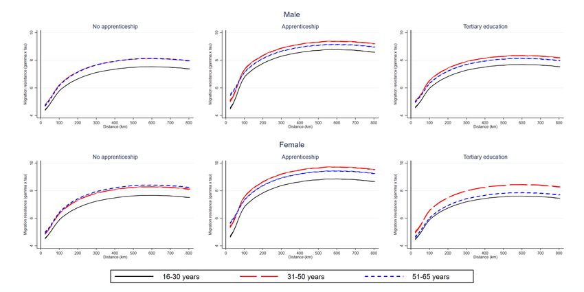
origin-destination-group component τijθ × γ θ , which we term migration resistance. There-
fore, the typically observed distance decay in migration flows can be rationalized by large
difference in migration cost if tastes are heterogeneous (small γ θ ) or small difference in
migration costs if tastes are homogeneous (large γ θ ).
It is immediate from Eq. (10) that there are isomorphic model formulations in which
θ
bilateral amenity shocks Bij,t are subsumed into time-varying migration costs, or vice
versa. Our parameterisation is motivated by the belief that differences in average migration
flows observed over 25 years in our data are most likely driven by fundamental determinants
of migration costs that hardly change over time, whereas deviations from the long-run
average most likely reflect the short-run effects of random events that tend to cancel out
over time.
C.4 Equilibrium
We take the structural parameters {α, β, ρ, ι, γ θ , κθ , Bij,t
θ , τ θ }, structural fundamentals
ij
θ , η , Aθ }, and labour and land endowments {L̄θ , T̄ } as exogenously given. We
{ψi,t i,t i,t t i
impose the following labour market clearing conditions:
X
L̄θt = Lθi,t (12)
i∈J
L̄θt . Therefore, labour supply, Eq. (11),
P
with the economy-wide labor endowment L̄t = θ
directly maps into region-group employment Lθi,t , regional employment Li,t = θ Lθi,t and
P
θ via the first-order condition of labour demand, Eq. (6). Likewise, we impose
wages wi,t
housing market clearing so that regional employment Lθi maps into rents pi,t via output
Xi,t according to Eq. (8) (see Appendix Section J.1). Trade with the rest of the world
clears the markets for tradable goods and capital inputs.
Transitory spatial equilibrium Frictional migration implies that shocks to structural
fundamentals lead to non-instantaneous adjustment in Lθi,t . The role of the TSE is to
rationalize unbalanced migration flows and non-stationary employment that are typically
observed in data.
Stationary spatial equilibrium Migration is spatially neutral if the sum of outflows
equals the sum of inflows for each location:
X X
χθij|i,t Lθi,t = χθji|j,t Lθj,t ∀ j ∈ J, θ ∈ Θ. (13)
j∈J j∈J
12This condition enforces that Lθi,t is stationary, but it does not rule out migration due
to idiosyncratic taste shocks. We assume that congestion forces dominate agglomeration
forces to ensure that all regions are populated. The latter is governed by κθ for each group
according to Eq. (6). The former works through the price for housing as described by
Eq. (8). The effect of changes in population on individual housing expenditure is given
by (1 − α)∂pi,t /∂Lθi,t . We relegate details to Appendix J.4 where we also show that the
economy converges to a unique SSE for given primitives. Since Eq. (13) is unlikely to hold
in data, we view the SSE as a counterfactual situation to which an economy observed in
a TSE would converge in the absence of further shocks.
Dynamic equilibrium For given structural parameters and structural fundamentals
the dynamic equilibrium of the model is referenced by a (J ×Θ) ×Zt vector of region-group-
year-specific employment Lθi,t , where Zt denotes the number of periods in the transition
period from a TSE in t to the SSE reached in t + Zt . Hence, the dynamic equilibrium
nests the SSE and all TSEs up to the period where the spatial economy has converged to
the SSE. For given structural fundamentals {ψiθt , ηi,t }, Lθi,t maps to (J × Θ) ×Zt vectors
θ and prices p
of wages wi,t i,t via the first-order condition of labour demand, Eq. (6), and
housing market clearing, Eq. (8).
Competitive spatial equilibrium Characteristic for the competitive spatial equilib-
rium is the absence of spatial frictions. Within our framework, we can remove frictions by
θ = 0). Since workers
setting preference shocks and migration costs to zero (aθki,t (ω) = 0, τki
optimally relocate across locations within any period, we can impose the standard spatial
equilibrium condition that workers are indifferent between locations. To this end, we set
the indirect utility equal to a group-time specific reservation utility Ūtθ .
!1−α
α θ
(1 − ι)wi,t
θ θ
Vi,t = (1 − ι)wi,t Aθi,t = Ūtθ (14)
pi,t
Hence, observed wages and rents directly map to a Rosen-Roback (RR) QoL measure
Aθi,t = qtθ p1−α θ θ
i,t /wi,t (where qt collects all group-period specific constants).
C.5 Worker expectations
In specifying how agents form expectations, there is a trade-off between foresight and
tractability. Desmet et al. (2018) develop a fully tractable DSM under static expecta-
tions, i.e. workers project current realizations of good and factor prices into the infinite
future. In contrast, Caliendo et al. (2019b) exploit Bellman’s principle to estimate model
parameters and conduct counterfactual analyses under perfect foresight without pinning
down all primitives. We marry both approaches with the aim of incorporating forward-
looking expectations into a model where all structural parameters and fundamentals will
be quantified.
13Our choices are guided by the stylized fact that the mean worker moves only once over
the entire employment biography (see Section B). Hence, we assume that workers do not
consider sequential moves when making migration decisions. For a formal derivation of
the expected region-group-period utility in the general case with sequential moves and the
special case with singular moves, we refer to Appendix J.3.
Workers who expect to remain at a migration destination forever likely form sophisti-
cated expectations with respect to the evolution of wages and rents. Therefore, we assume
that workers correctly anticipate the dynamic equilibrium referenced by the employment
vector Lθi,t and all model-endogenous adjustments in wages and prices summarized by wi,t
θ
and pi,t . Shocks to exogenous structural fundamentals cannot be anticipated, so workers
project observed realisation of QoL Aθi,t+1 into the future. Consistent with the distribu-
θ
tional assumptions in Eq. (4), workers expect a bilateral amenity E(Bi,j,t+s ) = 1 for s > 1.
In line with the conventions in DSMs, workers have an infinite time horizon and do not
expect to age.
C.6 Spatial arbitrage
The CSE is the urban economics equivalent of the no-arbitrage condition in financial
economics (Glaeser, 2008). Perfect spatial arbitrage is an assumption that leads to constant
reservation utility as a building block of neoclassical urban economics models. In contrast,
spatial arbitrage is an endogenous process in our DSM that moderates the transition from
the TSE to a SSE.
Intuitively, shocks to structural fundamentals affect expected utility directly or in-
directly. For example, a positive shock to labour productivity maps into higher wages
θ
wi,t+s according to Eq. (6) due to perfect competition on goods and labour markets and
the choice of the tradable good as the numeraire. Likewise, a positive shock to housing
productivity maps into lower housing costs pi,t+s according to Eq. (8) due to perfect
θ
competition among developers. Higher wi,t+s and lower pi,t+s affect bilateral migration
probabilities χθij|i,t according to Eq. (10), leading to in-migration. Given Eq. (11), this
results in endogenous changes in employment which in turn determine changes in wages
according to Eq. (6) and housing costs according to Eq. (8). As long as agglomeration
costs exceed agglomeration benefits at the margin, the consequence of migration is to
reduce the differences in expected utility that cause migration. The pace at which this
spatial arbitrage process takes place depends positively on the migration elasticity γ θ and
negatively on migration costs τijθ . Eqs. (10) and (11) establish how regions offering a
θ
greater indirect utility Vj,t+1 will experience larger net-immigration the larger γ θ and the
smaller the migration resistance τijθ × γ θ , ceteris paribus.
C.7 Quality-of-life premiums
The revealed-preference literature computes the value of amenities that jointly constitute
QoL via spatial differences in real living cost p1−α
i /wiθ , the inverse of the real wage (Rosen,
141979; Roback, 1982). Using the structural parameters and fundamentals quantified in
Section D, Figure 2 provides a graphical illustration of the simulated model to show how
QoL premiums are determined. Our case in point is the urban QoL premium which
captures how QoL depends on city size, a question that is controversially debated in the
literature (Albouy, 2011). To ease the presentation, we focus on the special case with one
worker group and refer to Appendix J.5 for formal derivations.
Intuitively, Figure 2 depicts two equilibrium loci in the real living cost-employment
space. The housing equilibrium locus (HS ) is a log-linearized version of Eq. (8) collecting
points that satisfy all housing-market related conditions that must hold in the TSE (and
the SSE). Under plausible parameterisations, the expenditure on housing increases faster in
city size (due to inelastically supplied land) than the wage (due agglomeration economies).
Therefore, the housing equilibrium locus is positively sloped. Greater housing productivity
ηi shifts the housing equilibrium locus downwards. Likewise, the migration equilibrium
locus (LS ) collects all points that satisfy all migration-related conditions that must hold
in the SSE. It is derived from Eq. (11). Intuitively, the migration equilibrium locus is
downward sloping since the preference of the marginal resident joining the city decreases
as city size increases due to taste heterogeneity (Arnott and Stiglitz, 1979; Moretti, 2011).
The slope of the migration equilibrium locus is inversely related to the migration elasticity
γ θ . Higher QoL Aθi shifts the migration equilibrium locus upwards. The intersection of
both equilibrium loci is the only combination of real wages and employment that satisfies
all SSE equilibrium conditions and, hence, we can use it to quantify the model and derive
QoL premiums.
The two vertical dashed lines mark two cities of different size. Housing productivity
ηi is higher in the larger city, which gives the city an edge in the competition for workers
since the housing sector provides more housing at the same equilibrium price (HS,1 is
below HS,0 ). Yet, despite the housing productivity advantage, the city size differential
can only be rationalized by a greater labour supply (defined by Eq. (11)) in the larger
city and an upward-shifted migration equilibrium locus (LS,1 vs. LS,0 ). Intuitively, the
lower idiosyncratic amenity of the marginal resident must be compensated for by a higher
average group-specific QoL Aθi in the larger city. Hence, there is a positive urban QoL
premium.
With decreasing taste heterogeneity, the migration elasticity γ θ increases, the slope of
the migration equilibrium flattens, and the urban QoL premium shrinks. For the limit
case γ θ →
− ∞, our model nests the canonical CSE framework in which the migration
equilibrium locus is simply a horizontal line shifted by Aθi (see Eq. (14)). In the given
example, because the larger city has a fundamental housing productivity advantage, we
qualitatively misrepresent the urban QoL premium if we abstract from taste heterogeneity.
The important takeaway is that urban QoL premium in the DSM with taste hetero-
geneity is necessarily more positive than in the canonical spatial equilibrium framework
unless the migration elasticity γ θ is large. More generally, we necessarily recover larger
QoL differentials from a model with taste heterogeneity. Since, consistent with the lit-
15erature (Caliendo et al., 2019b), we estimate relatively low values of γ θ for all groups,
we expect our quantitative framework to deliver larger valuations of local non-marketed
goods than the canonical Rosen-Roback framework.
Figure 2: The urban quality of life premium
Note: A formal derivation of demand and supply shifters and elasticities is relegated to Appendix A. We use
parameter values γ = 0.5 and β = 0.2 which are within the range of estimates in the literature and our own
estimates in Section D. We use the structural fundamentals quantified in Section D. To ease the presentation, we
derive all curves for one worker group (middle-aged, skilled male workers) exclusively.
D Quantification
The quantification of the model consists of two steps. First, we obtain values of the
structural parameters {α, β, ρ, ι, γ θ , ζ θ , κθ , Bij,t
θ , τ θ }.
ij We borrow {α, ι, ρ} from
the literature and estimate the remaining parameters using variables observed in data
{Lθi,t , T̄i , wi,t
θ , χθ
ij|i,t , pi,t } and the structure of the model. Second, we use data, the esti-
mated parameter values, and the structure of the model to invert the structural funda-
θ , η , Aθ } and to solve for the region-group-time-specific employment vector
mentals {ψi,t i,t i,t
Lθi,t that references the dynamic equilibrium.
D.1 Data
As an empirical correspondent to locations indexed by i in the model, we choose 141
German labour market regions defined by Kosfeld and Werner (2012) based on commuting
data. The centre of a labour market region is the municipality with the largest number
of workers. We treat periods t in our model as years in the data. We briefly discuss the
sources and processing of our data below and refer to Appendix K.1 for details.
16Employment Our measure of employment Lθi,t is constructed from the Employment
History (BeH) covering the years 1993-2017. This dataset is provided by the Institute of
Employment Research (IAB) and contains information on the universe of employees in
Germany (with the exception of civil servants and the self-employed) on a daily basis. We
only select those workers who are employed subject to social security contributions (includ-
ing apprentices) and compute region-year-specific employment levels for different groups
which are defined according to the interactions between sex, three skill categories (no ap-
prenticeship, completed apprenticeship and tertiary education) and three age categories
(16-30 years, 31-50 years and 51-65 years).
Migration We assign workers to labour market regions using their place of employment
θ are then constructed
as reported in the BeH. Bilateral group-specific migration flows Mij,t
by computing the number of workers belonging to group θ who were employed in region
i in year t, but who are working in region j in year t + 1 for every pair of origin region
i and destination region j. The conditional migration probabilities are then observed as
χθij|i,t = Mij,t
θ /Lθ .
i,t
Wages We follow the standard approach in labour and urban economics and identify
θ from movers by regressing individual wages against region-
the region-group-year wage wi,t
group-year fixed effects, controlling for individual fixed effects (Abowd et al., 1999; Combes
et al., 2008). We use matched employer-employee data including nominal wages from the
IAB covering the universe of German workers and establishments from 1993 to 2017.
Rents We follow Combes et al. (2019) and compute a house price index for a represen-
tative property at the centre of a labour market area. This index maps into rent pi via
a constant cap rate of 0.035 (Koster and Pinchbeck, 2018). The property micro data we
use is from Immoscout24 covering more than 16.5 million sales proposals for apartments
and houses between 2007-2017. The data were accessed via the FDZ-Ruhr (Boelmann and
Schaffner, 2019).
Geographic variables We use GIS to compute the land area T̄i of all regions and the
great circle distance between all pairs of regions. For a cultural distance measure, we use a
re-scaled version of the county-based dialect similarity index by Falck et al. (2012), which
we aggregate to labour markets.
Big data We use social media data from Facebook, Flickr, and Picasa to approximate
regional amenity value and social connectedness. We use those data to over-identify esti-
mated structural parameters and inverted structural fundamentals.
Location characteristic For our policy application, we compute the average concentra-
tion of particular matter (PM10 ) across municipalities. We also collect a comprehensive
17data set on fundamental first-nature characteristics that potentially affect productivity
(e.g. access to navigable rivers), amenity (e.g. opera houses, World War II destruction),
and housing TFP (e.g. physical constraints to development).
D.2 Structural parameters
We set the housing expenditure share to 1 − α = 0.33, which is in line with a literature
summarized in Ahlfeldt and Pietrostefani (2019) and official data from Germany (Statistis-
ches Bundesamt, 2020). We use a tax rate of ι = 0.49 which incorporates social insurance
contributions that are proportionate to income in Germany (OECD, 2017). Likewise,
we set the intertemporal discount rate to ρ = 0.11 following the economics literature on
time-preferences (Moore and Viscusi, 1988; Frederick et al., 2002). Lastly, we impose that
θ
stayers face no migration cost (τij=i = 0).
We estimate all other parameters using estimation equations that we derive from the
structure of the model. For identification, we generally follow the current best-practice
examples in the respective fields. Our main empirical contribution is to exploit our rich
data to account for greater inter-group heterogeneity than in previous work. We briefly
discuss the parameter values along with references to the identification strategies and the
relevant literature below. For a formal derivation of all estimation equations and full
estimation results we refer to Appendix K.2.
Density elasticity of productivity (κθ ) The estimating equation for κθ is a log-
linearized version of Eq. (5). Identification comes from between-labour-market-area
movers and is conditional on individual effects (Combes et al., 2008). We use a 100-year lag
of population density following a literature that argues that production fundamentals that
determined productivity in history are no longer relevant today (Ciccone and Hall, 1996).
With this approach, we estimate the agglomeration elasticity for Θ = 18 groups and find
that returns to agglomeration (κθ ) are not only biased with respect to skills (Baum-Snow
and Pavan, 2013), but also gender, with women benefiting more from agglomeration. The
weighted average elasticity estimate of 0.018 is close to the typical result in the literature
(Combes and Gobillon, 2015).
Land share (β) The estimating equation for β is a log-linearized version of Eq. (8). The
estimation equation is similar to the one in Combes et al. (2019), although, following from
our general equilibrium setting, the main dependent variable is GDP density rather than
population. Following the literature we, again, use the 100-year lag of population density
as an instrument. Our estimate of β = 0.18 implies a population density elasticity of house
prices of 0.2, which is within the typical range in the literature (Ahlfeldt and Pietrostefani,
2019). The implied intensive-margin housing supply elasticity (1 − β)/β = 4.2 is close to
existing structural estimates (Epple et al., 2010).
18Migration elasticity (γ θ ) The estimating equation for γ θ is a log-linearized and spa-
tially differenced version of Eq. (10) in which leading migration probabilities control for
future utility flows according to the Bellmann’s principle (Artuç et al., 2010). We follow the
literature and estimate γ θ using GMM. In our preferred approach, we restrict the identify-
ing variation to lagged group-specific average wage differences between eastern and western
states that likely capture a legacy of the cold-war era. The estimated average elasticity
of 0.3 is somewhat larger than when we use the standard IVs (lagged wage and migration
probabilities), but somewhat smaller than previous estimates for the U.S. (Caliendo et al.,
2019a). Novel to the literature, we find that middle-aged and middle-skilled male workers
are those that are most responsive to economic migration incentives.
Migration costs (τijθ ) The estimating equation for τijθ is a log-linearized version of
Eq. (10) using a PPML estimator. Destination-group-year and origin-group-year effects
control for arbitrary pull factors and multilateral resistance (Head and Mayer, 2014b).
Exploiting the panel-dimension, origin-destination-time effects non-parametrically identify
origin-destination-group-specific migration resistance τijθ × γ θ up to a constant. Exploiting
θ
the no-internal-migration-cost constraint τi,j=i = 0, we derive theory-consistent estimates
of τijθ for given values of γ θ . Female, old, and middle-skilled workers face largest resistance
to migrate. Yet, middle-skilled workers experience low migration costs. Because their
tastes are relatively homogeneous (large γ θ ), small differences in migration costs rationalize
large differences in migration flows. In monetary terms, the weighted average migration
cost corresponds to about e170K which is more than revealed in survey-based research
for the average U.S. citizens, though much less than for those who report themselves as
“rooted” (Koşar et al., 2019).
θ)
Bilateral amenity (Bij θ is the same gravity migration
The estimating equation for Bij
equation from which we infer migration resistance τijθ × γ θ . For given values of γ θ , we infer
θ from the structural residual. Consistent with theory, we rationalize migration flows of
Bij
θ = 0.
zero by setting Bij
D.3 Structural fundamentals
Labour and housing productivity Given our estimates of the agglomeration elasticity
κθ and observed wages wi,t
θ , regional employment
P θ
θ Li,t , and land area T̄i , we invert
fundamental labour productivity ψi,t using the first-order condition of labour demand,
Eq. (6). Likewise, we use our estimate of the land share β and observed rents pi,t , output
P θ θ
θ wi,t Li,t and land area T̄i to invert fundamental housing productivity ηi,t using housing
market clearing, Eq. (8).
Quality of life Owing to the dynamic structure of our model, the inversion of QoL Aθi,t
is less straightforward. Given observed data on conditional migration probabilities χθij|i,t
θ , migration costs τ θ and the migration elasticity
and estimates of bilateral amenities Bij,t ij
19You can also read