Optomechanics with Levitated Particles.
←
→
Page content transcription
If your browser does not render page correctly, please read the page content below
Optomechanics with Levitated Particles.
                                                            James Millen,1, ∗ Tania S. Monteiro,2 Robert Pettit,3 and A. Nick Vamivakas3
                                                            1
                                                              Department of Physics, King’s College London, Strand, London, WC2R 2LS, UK.
                                                            2
                                                              Department of Physics and Astronomy, University College London, Gower Street, London, WC1E 6BT,
                                                            UK.
                                                            3
                                                              The Institute of Optics, University of Rochester, 480 Intercampus Drive, River Campus, Rochester, NY 14627,
                                                            USA.
                                                            (Dated: January 23, 2020)

                                                            Optomechanics is concerned with the use of light to control mechanical objects. As a field, it
                                                            has been hugely successful in the production of precise and novel sensors, the development of
                                                            low-dissipation nanomechanical devices, and the manipulation of quantum signals. Micro- and
arXiv:1907.08198v2 [physics.optics] 22 Jan 2020

                                                            nano-particles levitated in optical fields act as nanoscale oscillators, making them excellent low-
                                                            dissipation optomechanical objects, with minimal thermal contact to the environment when op-
                                                            erating in vacuum. Levitated optomechanics is seen as the most promising route for studying
                                                            high-mass quantum physics, with the promise of creating macroscopically separated superposi-
                                                            tion states at masses of 106 amu and above. Optical feedback, both using active monitoring or
                                                            the passive interaction with an optical cavity, can be used to cool the centre-of-mass of levitated
                                                            nanoparticles well below 1 mK, paving the way to operation in the quantum regime. In addi-
                                                            tion, trapped mesoscopic particles are the paradigmatic system for studying nanoscale stochastic
                                                            processes, and have already demonstrated their utility in state-of-the-art force sensing.

                                                  ∗ Electronic   address: james.millen@kcl.ac.uk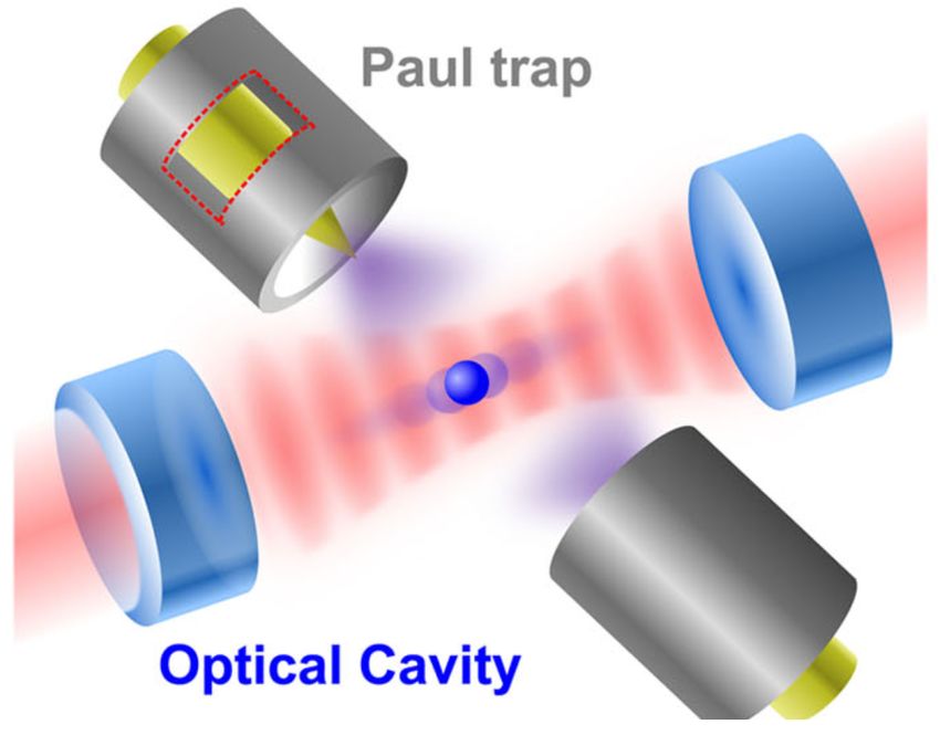
2

Introduction

   It is a pleasant coincidence, that whilst writing this review the Nobel Prize in Physics 2018 was jointly awarded
to the American scientist Arthur Ashkin, for his development of optical tweezers. By focusing a beam of light, small
objects can be manipulated through radiation pressure and/or gradient forces. This technology is now available off-
the-shelf due to its applicability in the bio- and medical-sciences, where it has found utility in studying cells and other
microscopic entities.
   The pleasant coincidences continue, when one notes that the 2017 Nobel Prize in Physics was awarded to Weiss,
Thorne and Barish for their work on the LIGO gravitational wave detector. This amazingly precise experiment is,
ultimately, an optomechanical device, where the position of a mechanical oscillator is monitored via its coupling to
an optical cavity. The field of optomechanics is in the ascendency [18], showing great promise in the development of
quantum technologies and force sensing. These applications are somewhat limited by unavoidable energy dissipation
and thermal loading at the nanoscale [62], which despite impressive progress in soft-clamping technology [209] means
that these technologies will likely always operate in cryogenic environments.
   Enter the work of Ashkin: in 1977 he showed that dielectric particles could be levitated and cooled under vacuum
conditions [16]. By levitating particles at low pressures, they naturally decouple from the thermal environment, and
since the mechanical mode is the centre-of-mass motion of a particle, energy dissipation via strain vanishes. The
field of levitated optomechanics really took off in 2010, when three independent proposals illustrated that levitated
nanoparticles could be coupled to optical cavities [21; 38; 185]. This promises cooling to the quantum regime, and
state engineering once you are there. This excited researchers interested in fundamental quantum physics, since it
seemed realistic to perform interferometry with the centre-of-mass of a dropped particle to test the limits of the
quantum superposition principle [186]1 .
   Simultaneously, Li et al. began pioneering studies into exploring nanoscale processes with levitated microparticles,
explicitly observing ballistic Brownian motion for the first time [118; 120]. It had already been realized that trapped
Brownian particles were paradigmatic for studying nano-thermodynamic processes [195], but the ability to operate in
low-pressure underdamped regimes, as well as to vary the coupling to the thermal environment (as offered in levitated
systems) inspired a slew of works, including the first observation of the Kramers turnover [188] and the observation
of photon recoil noise [100].
   This review is structured as follows: in Sec. I we outline the basic physics involved in levitating dielectric particles;
in Sec. II we briefly review the study of nanothermodynamics with optically levitated particles; in Sec. III we discuss
methods to use active feedback to cool the centre-of-mass motion; and in Sec. IV we illustrate the utility of the system
in force sensing.
   Moving onto quantum applications: in Sec. V we introduce levitated cavity optomechanics; in Sec. VI we discuss
potential tests of quantum physics using massive objects; and in Sec. VII we consider coupling to spins within levitated
nanoparticles. In Sec. VIII we cover some cutting-edge topics, before an outlook in the concluding Sec. IX.

Contents

        Introduction                                                                                                           2

     I. Optically trapped particles: the basics                                                                                4
        A. Optical forces and trapping geometries                                                                              4
        B. Equations of Motion                                                                                                 5
        C. Autocorrelation function, Power Spectral Density and c.o.m. Temperature                                             6

    II. Thermodynamics                                                                                                         7
           1. Brownian Motion:                                                                                                 8
           2. Thermally activated escape:                                                                                      8
           3. Heat Engines:                                                                                                    8
        A. Internal temperature                                                                                                9
           1. Absorption and emission:                                                                                         9
           2. Practical considerations and particle instability                                                                11

    III. Detection and Feedback Control                                                                                        11
         A. Detection and calibration                                                                                          11
            1. Calibration:                                                                                                    12
         B. Feedback Cooling                                                                                                   13

1   This has been proposed in a standard optomechanical system, but the experimental conditions required are daunting [129].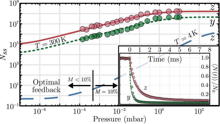
3

         1. Nonlinear feedback cooling:                                                     13
      C. Limits to feedback cooling                                                         13

 IV. Sensing                                                                                15
        1. Detection of surface forces                                                      16
        2. Sensing with levitated cavity optomechanics                                      17
     A. Other experimental configurations                                                   17
        1. Sensing via orientation:                                                         18
        2. Detection of static forces:                                                      18
     B. Exotic sensing schemes                                                              18

  V. Levitated Cavity Optomechanics                                                         19
     A. Levitated cavity optomechanics                                                      20
        1. The quantum back action (QBA) regime:                                            21
     B. Levitated cavity optomechanics: four challenges                                     22
           1. Maximizing the mechanical frequency:                                          22
           2. Maximizing the optomechanical coupling:                                       24
           3. Minimizing optical heating:                                                   24
           4. Minimizing gas heating; stable trapping at high vacuum:                       25
     C. Levitated cavity optomechanics: state of play                                       25
     D. Further physical studies possible with levitated cavity optomechanics               26

 VI. Tests of Quantum Physics                                                               26
     A. Interferometry                                                                      27
        1. Other interferometric schemes:                                                   28
     B. Decoherence                                                                         29
     C. Wavefunction collapse models                                                        31
        1. Dynamical reduction models:                                                      31
        2. Gravitational collapse models:                                                   33
     D. Preparing mechanical quantum states                                                 33

VII. Spin Systems (Nitrogen-Vacancy Centers in Diamond)                                     34
        1. The NV centre:                                                                   34
        2. Levitated nanodiamond:                                                           35

VIII. Further Topics                                                                        37
      A. Librational and rotational optomechanics                                           37
         1. Librational optomechanics:                                                      37
         2. Rotational optomechanics:                                                       39
      B. Novel cooling mechanisms                                                           40

 IX. Conclusion                                                                             42
     A. Discussion                                                                          42
        1. Comparison of levitated oscillators and state-of-the-art tethered oscillators:   42
        2. Comparison of feedback and cavity cooling:                                       43
     B. Outlook                                                                             43

      Acknowledgments                                                                       44

      References                                                                            44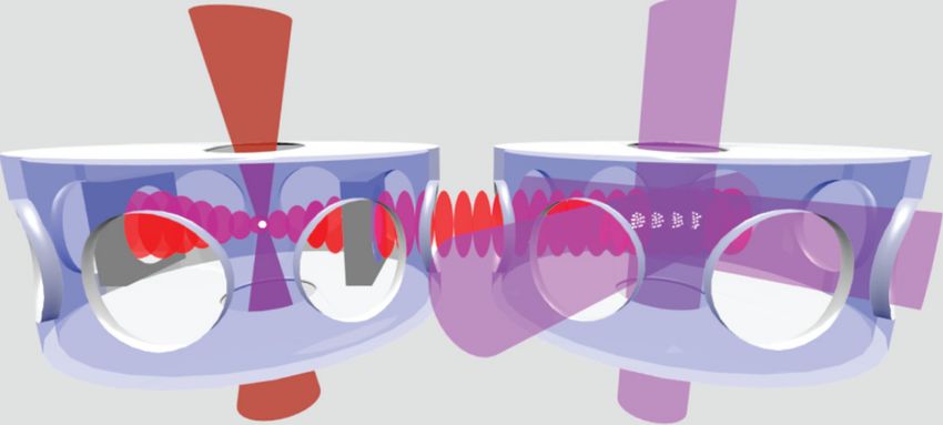
4
Levitated
Optomechanics
(c)
(b)
(a)
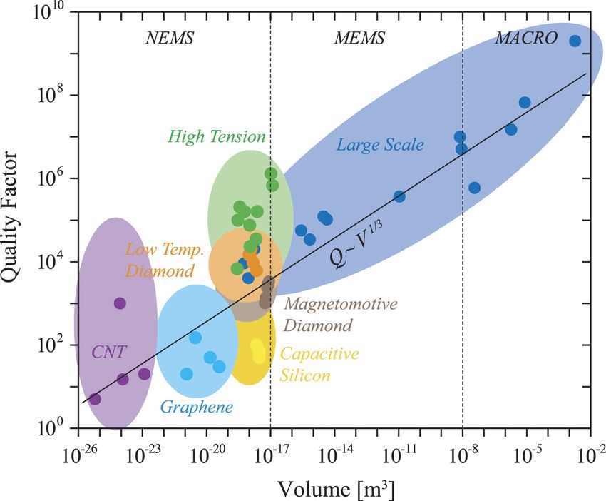
FIG. 1: Scaling of mechanical quality factor with oscillator volume, modified from [99]. The red shaded area represents the
range in which levitated optomechanical experiments are predicted to operate. Black points represent the state-of-the-art tethered
optomechanics experiments: (a) Ref. [209], (b) Ref. [74], (c) Ref. [123].
I. OPTICALLY TRAPPED PARTICLES: THE BASICS
To avoid limitations associated with mechanically tethered oscillators, levitation-based experiments have been
developed [38; 76; 106; 118; 144; 186]. In these experiments, the mechanical object is typically held by an intense optical
field rather than being tethered to the environment. In doing so, the primary dissipation comes from interactions with
the surrounding gas, which can be minimized by working in vacuum, and noise in the optical field. In levitation-based
experiments, the mechanical object is typically a micro- or nano-sized particle, with a geometry chosen to highlight
a specific type of motion. For example, while spherical particles are ideal for monitoring centre-of-mass motion,
ellipsoidal or cylindrical particles can be used to investigate rotation and libration [94; 112]. Particles can also be
fabricated from birefringent materials, providing further means to influence motion [10; 211].
An interesting comparison between levitated optomechanical resonators and traditional (tethered) opto- and electro-
mechanical resonators is made in Fig. 1. There is a general scaling of the tethered resonator’s quality factor pro-
portional to the cube root of the resonator’s volume. For levitated optomechanical systems this is not the case, and
quality factors well above the general trend can be achieved, as illustrated in Fig. 1. The variation in quality factor
with particle volume is due to the effects of gas-induced damping and photon recoil, see Sec. I.B. Oscillators of low
mass and high quality factor are particularly useful for force sensing. Also included on this figure are the state-of-
the-art tethered experiments, where engineering is used to minimize mechanical loss. A full comparison between the
quality factors of tethered and levitated systems is reserved for Sec. IX.
A. Optical forces and trapping geometries
We now describe a dielectric sphere of radius R
λ, where λ is the optical trapping wavelength, a regime where
we can neglect the radiation pressure force [77; 139]. The interaction of such a sphere with a light field of frequency
ωL = 2πc/λ is governed by the complex polarizability α(ωL ):
r (ωL ) − 1
α(ωL ) = 4π0 R3 , (1)
r (ωL ) + 2
where the frequency dependent permittivity is related to the complex refractive index through r (ωL ) = n(ωL )2 .
While the real part α0 determines the optical potential, the imaginary part α00 determines optical absorption, with
absorption cross-section σabs = ωL α00 /(c0 ).
5

  A particle can be confined by the optical potential formed by tightly focused light, a system which can be modelled
as a harmonic oscillator in three spatial dimensions. The acting gradient force can be expressed as

                                                                      α0
                                                        hFgrad i =       h∇E2 i,                                                   (2)
                                                                      2
where E is the electric field of the light. If we make the simplifying assumption that the focused beam is Gaussian
and assume that the particle occupies displacements small with respect to the beam waist and Rayleigh range, the
gradient force acting on the particle is well-approximated by a linear restoring force

                                                 hFgrad,q i = −kq q       q ∈ {x, y, z},                                           (3)

where the x and y coordinates are taken to be the degrees-of-freedom transverse to the direction of propagation of
the optical beam, and the z coordinate is parallel to the direction of propagation. For a description when the force is
non-linear, see Sec. II.
  The spring constants kq are different for each degree-of-freedom for a linearly polarized Gaussian beam

                                                                 4α0 Popt (t)
                                                         kq =                  ,                                                   (4)
                                                                πc0 wx wy wq2
                                                                                                               √
where wq is the beam waist along the q-direction, wz is related to the Rayleigh range z0 through wz = 2z0 , and
Popt (t) is the power contained within the optical beam1 . Time dependence has been included in the power term to
hint at the possibility of controlling particle dynamics through this variable; the ability to dynamically vary the spring
constant is a key advantage of optically levitated oscillators.

B. Equations of Motion

   The linear restoring force in eqn. (3) indicates that we can construct the equation of motion for each degree-of-
freedom q of the particle’s center-of-mass (c.o.m.) in the following way

                                        M q̈(t) = −M ΓCM q̇(t) − M ωq2 q(t) +
                                                                                   p
                                                                                    2πSff η(t),                                    (5)
             p
where ωq = kq /M is the mechanical oscillation frequency of the trapped particle, ΓCM is the total momentum
damping rate acting on the particle, and M is its mass. Sff is the force spectral density associated with coupling to
a bath at temperature Tenv at a rate ΓCM , such that 2πSff = 2M kB Tenv ΓCM , and η(t) encodes a white-noise process,
such that hη(t)i = 0, hη(t)η(t0 )i = δ(t − t0 ). This model holds as long as the dynamics are linear, i.e. the oscillation
amplitude of the particle in the optical trap is small. Nonlinear contributions to the motion are negligible under the
condition [78; 139]

                                                           3kB TCM
                                                           2
                                                                           1,                                                     (6)
                                                          wq ΓCM ωq M

where TCM is the temperature of the c.o.m. (which may differ from Tenv ). When this condition is not met, the
different motional degrees-of-freedom are no longer independent [78]. There is a further discussion of nonlinearities
in Sec. II.
   The momentum damping rate of a levitated oscillator in ambient or low-vacuum conditions is dominated by collisions
with the background gas ΓCM ≈ Γgas . For a spherical particle in a rarefied gas, the damping rate is [139]

                                                        6πηgas R    0.619
                                               Γgas =                       1 + cK ,                                               (7)
                                                          m      0.619 + Kn

1   For a nanoparticle trapped in a standing-wave formed by counter-propagating beams of equal polarization, or the field of an optical
    cavity, the axial spring constant is kz = 2α0 kL
                                                   2P
                                                      opt (t)/πc0 wx wy , where kL is the wavenumber of the trapping light.
6

where ηgas is the dynamic viscosity of the background gas ηgas = 18.27 × 10⁻⁶ kg (ms)−1 for air, Kn = lgas /R is the
Knudsen number, given by the ratio of the mean free path lgas of the background gas to the radius of the trapped
particle, and cK = 0.31Kn/(0.785 + 1.152Kn + Kn2 ). When Kn  1, known as the Knudsen regime, the damping is
linearly proportional to pressure
                                                     r
                                                 8        2mgas 2
                                       ΓKn>1
                                        gas  =                   R Pgas .     (Low pressure)                         (8)
                                                 3       πkB Tim
The transition to the Knudsen regime occurs at a pressure Pgas ≈ 54.4 mbar/R(µm). Mechanical quality factors
Qm = ωq /ΓCM range from ∼ 10 at 10 mbar to ∼ 108 at 10−6 mbar.
   Another stochastic force which an optically trapped particle experiences is that due to the discrete photon nature
of light, known as photon shot noise. This has been recently measured [100], and leads to a damping rate [85; 139]

                                                                cdp Pscat
                                                          Γrad =          ,                                           (9)
                                                                  M c2
where cdp depends on the motion of the particle relative to the polarization of the light (cdp = 2/5 for motion parallel
to the polarization, cdp = 4/5 for motion perpendicular to the polarization), and Pscat is the power of the light
scattered by the particle. This depends upon the polarizability of the particle α, the wavevector kL and intensity
Iopt of the trapping light: Pscat = |α|2 kL4 Iopt /6π0 2 . In general, Γrad  Γgas until pressures below ∼ 10−6 mbar are
reached, at which point it becomes the dominant damping mechanism. The total damping rate ΓCM is the sum of all
the different momentum damping rates.
  A nanoparticle exposed only to photon shot noise would reach an equilibrium temperature given by the photon
energy [100], TCM = ~ωL /2kB . This temperature is in general very high, and necessitates continuous additional
cooling (i.e. active feedback, Sec. III or passive cavity cooling, Sec. V) to stabilize optically trapped nanoparticles
at low pressures. Figure 3 later in the manuscript illustrates the implication of the competing heating and damping
mechanisms on the c.o.m. temperature.

C. Autocorrelation function, Power Spectral Density and c.o.m. Temperature

  It is not always straightforward to directly analyse eqn. (5) due to the stochastic term. The first tool we will
consider is the position autocorrelation function (ACF) hq(t)q(0)i for the position variable q(t):

                                                                 kB TCM  1
                                               hq(t)q(0)i =             − σq2 (t).                                  (10)
                                                                  M ωq2  2
In the underdamped regime (ΓCM < ωq ), the position variance σq2 (t) is given by

                                        2kB TCM      − 21 ΓCM t               ΓCM
                            σq2 (t)   =          1−e              cos(ωq t) +     sin(ωq t) .                       (11)
                                         M ωq2                                2ωq
For a discussion of the autocorrelation function in different damping regimes, and between different variables, see
[139]. The c.o.m. temperature of the particle can be extracted from the t = 0 value of hq(t)q(0)i. Examples of
hq(t)q(0)i for different pressures and temperatures are shown in Fig. 2a), c).                   R∞
  The position ACF is the Fourier transform of the power spectral density (PSD) Sqq (ω) = 2π   1
                                                                                                  −∞
                                                                                                     hq(t)q(0)ie−iωt dt,
and is a convenient tool for analysing the response of the different degrees-of-freedom in frequency space. It is given
by

                                                               ΓCM kB TCM /πM
                                               Sqq (ω) =                              .                             (12)
                                                             (ω 2 − ωq2 )2 + Γ2CM ω 2
Examples of the PSD at different pressures and TCM are shown in Figs. 2 b), d). It is common to acquire Sqq (ω)
Rexperimentally,  and fit the data to eqn. (12) to extract TCM [90; 137]. Another method is to note that hq(0)q(0)i =
  ∞
     S (ω)dω, with hq(0)q(0)i = kB TCM /M ωq2 , i.e. by integrating over the PSD one can also extract the c.o.m.
  −∞ qq
temperature.
   This analysis assumes that the motion of the trapped particle is linear, whereas in the underdamped regime the
particle may undergo non-linear dynamics, as discussed in Sec. II. It is still possible to extract the energy of the
particle in this regime by analysing the PSD, see [78; 139].
7

FIG. 2: Autocorrelation functions (ACF) and Power Spectral Densities (PSD) in the underdamped regime Simulated a)
ACF and b) PSD at a gas pressure of 50 mbar for TCM = 1000 K (red) and TCM = 300 K (blue). Simulated c) ACF and d) PSD at a gas
pressure of 1 × 10⁻³ mbar with the same TCM as above (oscillations not resolved). Simulations are for an R = 100 nm silica sphere with a
mechanical frequency ωx = 2π × 100 kHz. Example experimental e) ACF and f) PSD of a levitated R = 105 nm silica sphere at 1 mbar.
Points are data and solid lines are fits based on eqns. (10) & (12). In f), the trapping laser intensity sets TCM , leading it to increase from
left-to-right (along with an increase in trapping frequency). Reproduced using the data from [137].

II. THERMODYNAMICS

   Trapped mesoscale objects are excellent test-beds for a range of thermodynamic phenomena. For a thorough
discussion of using levitated nanoparticles to investigate thermodynamics, see recent reviews by Gieseler & Millen
[77; 139].
   A nano- or micro-particle levitated in an optical trap couples to the thermal bath provided by collisions with the
surrounding gas. The motional energy of the particle is comparable to that of the thermal fluctuations of the bath: a
1 µm diameter silica sphere weighs ∼ 10−15 kg, and has velocities in an optical tweezer of ∼ mm s−1 , which at room
temperature (Tenv = 300 K) yields a kinetic energy of ∼ kB Tenv . With optical trap depths > 104 K, this means that
the motion of micron-sized particles is sensitive to thermal fluctuations, but not destructively so. Unlike macroscopic
thermal systems, or microscopic systems with relevant internal degrees-of-freedom, considering only the centre-of-mass
(c.o.m.) motion is sufficient to fully describe their behaviour2 .
   Working in a gaseous environment gives us the ability to dynamically vary the coupling to the bath by changing the
pressure. Hence, one has access to underdamped dynamics, as opposed to the overdamped dynamics always observed
in a liquid. One way to define the transition between these regions is to compare the harmonic frequency ωq of a
trapped particle to the momentum damping rate ΓCM , such that dynamics are underdamped when ΓCM
8
1. Brownian Motion:
Monitoring the Brownian motion of an object is an excellent window into an archetypal stochastic process. We
consider a single coordinate q(t). For a full discussion of the dynamics when the particle is harmonically trapped,
see [120]. The Langevin equation for a free particle, where the dominant noise process is due to collisions with gas
molecules, is
q
M q̈ + M Γgas q̇ = 2πSffgas η(t), (13)
with terms defined after eqn. (5). The mean squared displacement (MSD) for such a particle is
2kB Tenv
hq(t)2 i = (Γgas t − 1 + e−Γgas t ). (14)
M Γ2gas
To explore this result, we note that the relevant timescale is the momentum relaxation time τ = 1/Γgas . On long
timescales t
τ , eqn. (14) approximates to hq(t)2 i = 2k B Tenv
M Γgas t, which is the diffusive motion as predicted by Einstein.
On short timescales t
τ , eqn. (14) approximates to hq(t)2 i = kBM Tenv 2
t , which describes ballistic motion. The
transition from diffusive to ballistic motion is set by the gas pressure (via τ = 1/Γgas ), with the particle motion being
ballistic at low pressures. The first ever observation of the transition from diffusive to ballistic dynamics was made
using a levitated particle by Li et al. [118].
Brownian motion can cause a trapped nanoparticle to explore nonlinear regions of the trapping potential, as observed
by Gieseler et al. q
[78]. It is normally assumed that excursions of the oscillator are small, with the thermal amplitude
of motion ath
q = 2kB TCM /(M ωq2 ) < R, and hence we can consider the potential to be harmonic. However, for a
high-Qm oscillator, this no longer holds, and the different degrees of freedom q = {x, y, z} are no longer decoupled.
For an optical tweezer, in the directions transverse to the beam propagation direction, the dominant nonlinearity is
the cubic “Duffing” term [78; 80], and the Langevin equation reads
X q
M q¨i + M Γgas q˙i + M ωi2 qi + ξj qj2 qi = 2πSffgas η(t), (15)
j=x,y,z
where ξi is the nonlinear coefficient in the i = (x, y, z) direction, which in an optical tweezer can be approximated as
ξi = −1/wi2 . The consequence
P of this nonlinearity is that the mechanical frequency is not constant, and is red-shifted
by an amount ∆ωi = 83 ωi j ξj a2j , where ai is the instantaneous oscillation amplitude in the corresponding direction.
This frequency shift broadens and skews the power spectral density [78]. When ∆ωi
Γgas the nonlinear term can
be neglected.
2. Thermally activated escape:
We have discussed the dynamics of a particle confined within a potential, and subject to fluctuating forces from
the environment. Due to the stochastic nature of the imparted force, there is a probability that the particle will gain
enough energy to escape the potential, even when it is confined by a potential much deeper than kB Tenv , in a process
known as Kramers escape. It is often physically relevant in Nature to consider the stochastically driven transition
between two states, for example the transition between different protein configurations. In the underdamped regime,
the transition rate increases with increasing friction, and in the overdamped regime the transition rate increases with
decreasing friction, with the transition region labelled the turnover. The Kramers turnover was first experimentally
measured using a levitated nanoparticle hopping between two potential wells formed by focused laser beams [176; 188],
exploiting the fact that the friction rate can be varied over many orders of magnitude through a change in the gas
pressure Pgas .
3. Heat Engines:
When considering a nano-scale engine, the work performed per duty cycle becomes comparable in scale to the
thermal energy of the piston, and it is entirely possible for the engine to run in reverse for short times, due to the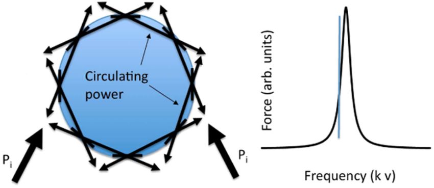
9

fluctuating nature of energy transfer with the heat bath. This is the scale at which biological systems operate, and a
regime which levitated nano- and micro-particles have access to.
   There have been many realizations of the overdamped heat engine [131], where the construction of optimized
work-extraction protocols is simplified, since the equations of motion are such that the position is independent of
the velocity. An analytic solution to the optimization problem is not possible in the underdamped case, where the
position and velocity variables cannot be separated [50; 83], and numerical methods must be used. In both regimes,
the optimum protocols call for instantaneous jumps in some control parameter [83], such as the trap stiffness, which
is easier to realize in the underdamped regime due to the rapid response of the particle.
   It seems challenging to realize an underdamped (levitated) stochastic heat engine when by definition coupling to
the heat bath (surrounding gas) is weak. Dechant et al. propose a realization of an underdamped heat engine, based
on an optically levitated nanoparticle inside an optical cavity [49]. In this case, the heat bath is provided through
a combination of residual gas (1 mbar) and the interaction with the optical cavity, which can cool the motion of the
particle.

A. Internal temperature

                                                                                            (q)
  So far in this review, when we discuss temperature, we refer to the c.o.m. temperature TCM = M ωq2 hq 2 i, which can
be changed from the ambient temperature Tenv through feedback (Sec. III) or cavity cooling (Sec. V). In this section
we discuss the role of the internal, or bulk, temperature of the particle Tint . For simplicity, we will consider the
particle to have a uniform temperature, though Millen et al. [137] observed an anisotropic temperature distribution
across the surface of silica microspheres due to internal lensing.
  It is well documented that the bulk temperature of a levitated particle affects its dynamics. Absorbing particles
are repelled from optical intensity maxima through the photophoretic effect [117]. In this process, the particle is
anisotropically heated by absorbing light. When gas collides with the particle, it sticks for some time to the surface,
and then leaves, converting some of the surface heat into momentum. The departing gas molecule imparts momentum
to the particle, giving it a kick. Hence, there is a stronger kick away from the hot surface, and the particle moves
away from the region of high light intensity. By employing complex optical beam geometries, the photophoretic effect
can lead to stable trapping and manipulation [197].
  The process by which a surface exchanges thermal energy with a gas is called accommodation, which is characterized
by the energy accommodation coefficient

                                                         Tem − Tim
                                                  αC =              ,                                             (16)
                                                         Tint − Tim
where Tim is the temperature of the impinging gas molecules and Tem the temperature of the gas molecules emitted
from the surface after accommodation. Accommodation quantifies the fraction of the thermal energy that the colliding
molecule removes from the surface, such that αC = 1 means the gas molecule fully thermalizes with the surface.
   When in the Knudsen regime (see Sec. I), the impinging gas molecules thermalize with the environment rather than
the emitted gas, such that Tim ≡ Tenv (6= Tem ). In this regime, the particle is subject to two independent fluctuating
thermal baths, one provided by the impinging gas molecules at Tim , and one by the emitted molecules at Tem . This
non-equilibrium situation can be characterized by an effective c.o.m. temperature [137]

                                                      Tim Γim + Tem Γem
                                              TCM =                     ,                                         (17)
                                                             Γtot
with a damping rate Γtot = Γim + Γem . Generally,
                                           p        Γim is given by eqn. (7) from the previous section. The damping
                                      π
rate due to the emitted gas is Γem = 8 Γim Tem /Tim . Note that Γem depends on Tint through eqn. (16), as has been
observed [137].
  Practically, when one analyses the motion of the particle, for example via the power spectral density, one will
measure TCM and ΓCM . Recent work has demonstrated a shift of a few percent in the trapping frequency ωq with
Tint , due to the dependence of the material density and refractive index upon temperature [90].

1. Absorption and emission:

  The bulk temperature of a levitated particle depends on several competing processes: heating through optical
absorption of the trapping light and optical absorption of blackbody radiation, and cooling through blackbody emission
10

              a)                                                                  b)
                                 700                                                                  5000
                                                                    Tint                                                                Tint

               Temperature (K)

                                                                                    Temperature (K)
                                 600                                                                  4000
                                                                    TCM                                                                 TCM
                                 500                                                                  3000
                                 400                                                                  2000
                                 300                                                                  1000

                                  10 -10                         10 0                                   10 -10                        10 0
                                           Pressure (mbar)                                                          Pressure (mbar)
FIG. 3: Interaction of internal and centre-of-mass temperatures. Variation in the bulk temperature Tint (solid lines) and
centre-of-mass temperature TCM (dot-dashed lines) with pressure for a) R = 10 nm, and b) R = 100 nm silica spheres, with
Tim ≡ Tenv = 300 K. These dynamics are due to the balance between optical absorption, blackbody absorption and emission (eqn. (18)),
photon recoil heating (eqn. (9)), and cooling due to collisions with gas molecules (eqn. (19)). This figure assumes a sphere trapped with
a realistic laser intensity of 6 × 10¹¹ W m−2 at a wavelength of 1550 nm. The optical trap depth is a) U0 /kB = 520 K and b)
U0 /kB = 5 × 10⁵ K. For silica we use a complex refractive index n = 1.45 + (2.5 × 10⁻⁹ )i [26], material density ρ = 2198 kg m−3 , and we
assume the surrounding gas is N2 , with a corresponding surface accommodation coefficient αC = 0.65.

and energy exchange with the background gas. The rate at which a sphere absorbs or emits blackbody energy3 is
given by [38]

                                                                           24ξ(5) 00
                                                             Ėbb,abs =               α (kB Tenv )5
                                                                          π 2 0 c3 ~4 bb
                                                                                                                                               (18)
                                                                               24ξ(5) 00
                                                            Ėbb,emis   = − 2 3 4 αbb     (kB Tint )5 ,
                                                                            π 0 c ~
where ξ(5) ≈ 1.04 is the Riemann zeta function, and αbb is averaged over the blackbody spectrum, such that for silica
 00
αbb ≈ 4π0 R3 × 0.1 [38]. Next we consider the cooling power due to collisions with gas molecules [38]

                                                                r
                                                                     2                γsh + 1                    Tint
                                                Ėgas = −αC            (πR2 )Pgas vth                                 −1 ,                     (19)
                                                                    3π                γsh − 1                    Tim

where vth is the mean thermal velocity of the impinging gas molecules and γsh = 7/5 is the specific heat ratio of a
diatomic gas. This expression holds in the Knudsen regime. Combining all of these leads to a rate equation that
describes Tint

                                                    dTint
                                           M cshc         = Iopt σabs + Ėgas (Tint ) + Ėbb,abs + Ėbb,emis (Tint ),                          (20)
                                                     dt
where cshc is the specific heat capacity for the particle material. Using eqn. (20), one can calculate the steady state
temperature of a sphere levitated in vacuum. It is possible to reach extremely high temperatures: Silica levitated at
1 mbar has been observed to reach its melting point at 1,873 K, and gold nanoparticles reach 1000s K at atmospheric
pressure [101]4 .
  The variation in Tint and TCM with pressure for different sized particles is shown in Fig. 3.

3   This assumes that the sphere is much smaller than typical blackbody radiation wavelengths, which is true for sub-micron particles.
4   The absorption of gold is greatly enhanced by the presence of plasmonic resonances.
11
2. Practical considerations and particle instability
It is clear from eqn. (20) that the material properties greatly effect the thermal behaviour of levitated particles,
and from eqn. (18) that both the optical absorption and emission rates depend on the absorption cross-section
σabs = ωL α00 /(c0 ). This means that low absorption materials also radiate their heat away slowly. This may be
of consequence when working in ultra-high vacuum, or during protocols where the trapping light is switched off for
periods of time.
One can measure the internal temperature Tint by monitoring the c.o.m. dynamics, as discussed above. Another
method is to use a material that emits light with a temperature dependent spectrum. For levitated nanoparticles,
this method has been used to estimate the temperature of nanodiamonds through measurement of the NV− centre
fluorescence [93], and the temperature of nanocrystals of YLF through measurement of the spectrum of Yb3+ impu-
rities [166]. There are a whole host of tracers and dyes that could be employed to do the same task [33]. It is also, in
principle, possible to directly measure the blackbody spectrum of a levitated nanocrystal [33].
At this point it is worth asking whether increases in internal temperature Tint , which affect the c.o.m. temperature
TCM , are enough to explain the widely reported problem of particle escape from optical traps at low pressures
[137; 171]. This is not a simple question to answer, as TCM depends on a balance between blackbody absorption
and emission (eqn. (18)), cooling from the surrounding gas (eqn. (19)), and further heating due to photon recoil
[100] (eqn. (9)), which in turn depend sensitively on the particle size and shape. In Fig. 3 we show some indicative
examples of the trade-off between these processes. We also note that recent work [203] has shown that circularly
polarized light can cause particles to undergo unstable orbits, which could play a role in regimes of low damping and
imperfect polarization control.
III. DETECTION AND FEEDBACK CONTROL
In this section, we consider methods for detecting the motion of optically trapped particles. This information can
then be used to control the motion of the particles via feedback. We focus on the use of feedback to extract energy
from the levitated oscillator, but note that feedback can also be used to study non-linear processes, such as phonon
lasing [159].
A. Detection and calibration
The ease of detection of a levitated nanoparticle depends strongly on its size. As briefly mentioned in Sec. I, the
power of the light scattered by a sub-wavelength sphere within an optical field is
Pscat = |α|2 kL4 Iopt /6π0 2 . (21)
Note that Pscat ∝ α2 ∝ R6 , so the amount of light it is possible to detect rapidly drops with particle radius. The
scattered light depends upon the local intensity Iopt , and so varies as the particle moves through the spatially varying
intensity profile of a focussed laser beam, yielding position sensitivity. This also means that position resolution
is improved by using tightly focussed beams, and using a standing wave increases resolution along the z-direction
(Fig. 4a)). Anisotropic particles have polarizabilities that vary with their alignment relative to the polarization vector
of the light field, meaning that Pscat is alignment-dependent [111; 112].
The scattered light can be collected using a lens and imaged onto a photodetector [138], or by placing a multi-mode
optical fiber close to the trapping region [111; 112], see Fig. 4a). The collected signal contains information about
all degrees-of-freedom, which can be analysed separately in frequency space. To collect information about different
degrees-of-freedom separately, the scattered light can be imaged onto a quadrant photodiode [137; 170; 171], or onto
a camera. The latter method is generally low bandwidth, though is suitable for low frequency oscillators and has
favourable noise characteristics [35; 198]. It is possible to use a fast camera and stroboscopic illumination to achieve
acquisition rates above 1 MHz [11].
A highly sensitive method for detecting nanoparticles is to make an interferometric measurement of position [167].
This method was pioneered with levitated particles by Gieseler et al. [76], and has enabled ∼ 1 pm Hz−1/2 position
sensitivity. The light which the particle scatters interferes with the trapping light. Collecting this pattern with a lens
produces an image of the momentum distribution of the particle. The trapping light acts to amplify the scattered-light
signal, as familiar from other homodyne detection techniques. For small oscillations (i.e. in a linear optical potential),
this technique produces a signal for motion in the q-direction proportional to Escat Eref q/wq , where wq is the beam12
a) b) c)
Detector
Superconducting
particle
Balanced
Lens detector - - - - - -
+++
+ +
++ +
+ + + + + +
Charged
Fiber particle
FIG. 4: Particle detection a) The light scattered from an optically trapped particle contains information about its position. This light
can be collected by a lens, a multimode fiber, or an optical cavity (not shown). b) The interference between the scattered light and the
trapping light acts as a homodyne measurement of the particle’s position when measured with a balanced detector. c) Non-optically
trapped particles can be detected by other means: charged particles induce a current in nearby electrodes (left) [82], and
superconducting particles induce a current in anti-Helmholtz pick-up coils (right) [184].
waist in the q-direction, as defined in Sec. I. The fields are those incident upon the detector, with Escat being the field
scattered by the particle, and Eref being the field due to the trapping light. For more details see Ref. [76].
The total intensity of the pattern at a fixed plane is proportional to the z-position only, and to measure the x, y-
positions one spatially splits the beam and makes a balanced detection, as illustrated in Fig. 4b), which removes the
intensity modulation due to the z-motion5 . Due to the dependence on the beam waist, optimal application of this
method requires the use of high numerical aperture trapping optics. The limiting factors of this technique are the
collection efficiency of the scattered light, and detector noise, see Ref. [204] for a thorough discussion.
The collection efficiency could be improved by using optical microcavities. Recently, such microcavities [213] have
been used to detect the motion of free nanoparticles [114], and the near-field of a photonic crystal cavity has been
used to detect the motion of a levitated nanoparticle [124], achieving a position sensitivity of ∼ 3 pm Hz−1/2 .
Macroscopic optical cavities can also be used to detect particle motion [15; 106], as also discussed in Sec. IV..2.
This currently represents the state-of-the art detection method, providing position measurement at the 10−14 m Hz−1/2
level [37; 221]. When working with such cavities, their narrow bandwidth should be taken into consideration.
A final set of detection methods are non-optical, Fig. 4c). Once could use inductive detection of charged nanopar-
ticles [82], which is predicted to be able to resolve displacements below 1 pm and detect sub-nm sized particles. This
method also gives direct access to the velocity of the particle, which is useful for feedback cooling, as discussed below.
It is also proposed to detect magnetically levitated superconducting spheres via pick-up coils [184].
1. Calibration:
Once the particle has been detected, the detected signal must be converted into position, i.e. the detector must be
calibrated. This is a significant source of uncertainty in many experiments.
The standard method is to analyse the PSD or the position variance, as discussed in Sec. I.C, and use the equiparti-
tion theorem to calibrate the detector. The limitations of this method are that it assumes the particle is in equilibrium
with its environment, which is often not true [90; 137], and that the motion of the particle is purely harmonic, which
is also often not true [78] (though this can be compensated for [88]). This method requires accurate knowledge of
the local temperature, and the pressure in the vicinity of the particle (which can only be measured to 10% accuracy
or worse). The mass of the particle must be known, which in principle can be inferred by measuring the damping
rate, but this requires confidence on the particle shape and density (and again the local pressure), and so represents
at least another 20% uncertainty. In addition, it has been found [88] that detector calibration is pressure dependent.
In all, there is a 20-30% uncertainty on detector calibration via analysis of the thermal motion of a levitated particle,
as discussed in more detail in [88].
It is possible to use another calibrated force to calibrate a detector, for example an electric force acting on a
charged particle [88; 92], but this requires a precise knowledge of the applied force. One can exploit particles trapped
5 particle rotation has also been detected using this method [2; 175].13
in optical standing waves, since the well-defined optical wavelength acts as a kind of ruler to calibrate the motion
of the particles as they cross nodes in the field [111; 112; 171], but this requires a detection method with a wide
field-of-view compared to the nm-level thermal motion of a trapped particle. Finally, it is possible to use a heterodyne
measurement to extract various experimental parameters, such as the damping, with high precision [48; 212].
B. Feedback Cooling
By detecting the motion of a levitated particle, feedback methods can be utilized to extract energy from each
degree-of-freedom. Such cooling is of great interest in the quest to reach the quantum regime of motion, see Sec. VI.
Feedback cooling can also be used to ensure that the particle does not oscillate with large amplitudes, which would
introduce nonlinear dynamics (as discussed in Secs. I & II), limiting the force sensing capabilities of the levitated
particle, see Ref. [78] and Sec. IV. Such cooling has proven invaluable for operating under high-vacuum conditions,
where it is necessary to stabilize the motion of the particle to prevent loss from the optical potential, see Sec. II.
The most general modification to the dynamics of a levitated particle can be described by adding a feedback term
ufb (t) to the Langevin equation [45]
p
2πSff
q̈(t) + ΓCM q̇(t) + ωq2 q(t) = η(t) + ufb (t), (22)
M
where q is one degree-of-freedom, and all other terms are defined after eqn. (5). By engineering a feedback term
proportional to the particle’s velocity ufb (t) = Gq̇ q̇(t), with some optimized gain Gq̇ [45], energy will be extracted
from the particle’s motion. This is referred to as “cold damping”, since it damps the motion of the particle without
introducing additional heating (dissipation without fluctuation). The addition of a term proportional to position
ufb (t) = Gq q(t) + Gq̇ q̇(t) leads to an increased cooling rate, but not a lower final temperature.
Such an active feedback mechanism was used to stabilize the motion of levitated microparticles (R ≈ 4 µm) as early
at 1977 by Ashkin [16]. Feedback cooling came into prominence after work by Li et al. [119], who used a 3-beam
radiation pressure scheme to cool the motion of a R = 1.5 µm sphere to 1.5 mK. The radiation pressure force drops
rapidly with size, so this protocol isn’t suitable for cooling particles smaller than ∼ 1 µm.
Recently, two groups have employed linear feedback cooling on 100-200 nm diameter charged particles using the
Coulomb force [45; 204] . An optical signal is used to generate an electrical feedback signal which is applied to
electrodes in the vicinity of the optically levitated nanoparticle. This has been used to generate temperatures in a
single degree-of-freedom as low as 100 µK, which represents less than 20 motional phonons [204].
1. Nonlinear feedback cooling:
In cases where it is desirable to work with both small and charge-neutral particles, it is most effective to utilize
the gradient force. In 2012, Gieseler et al. [76] presented influential work where parametric feedback cooling was
used to reduce a R = 70 nm nanoparticle’s centre-of-mass (c.o.m.) temperature to 50 mK. This involved a parametric
modulation of the trapping potential, with the feedback signal generated either by the trapping light (as in Fig. 4b)),
or by a probe beam. The phase of the feedback signal is tuned such that as the particle travels away from trap-centre
the potential is stiffened, and as it travels towards trap-centre the potential is relaxed. Such a scheme therefore
modulates the potential at twice the frequency of oscillation, which is achieved via ufb (t) = Gnl q(t)q̇(t).
This feedback process leads to damping on the particle motion δΓ ∝ Gnl hnm i, where nm is the number of motional
phonons. The power of the feedback cooling is a function of the oscillator amplitude, and hence it is referred to
as nonlinear feedback cooling. In linear damping schemes, as discussed above, the feedback damping rate δΓ is
independent of the oscillator energy.
Parametric feedback can be performed on all motional degrees-of-freedom simultaneously, since the gradient optical
force always points towards the trap centre. Signals from all degrees-of-freedom are summed together and delivered
to a device which actuates the trapping potential, such as an electro-optic modulator. Figure 5a) outlines a typical
experimental implementation of the feedback loop.
C. Limits to feedback cooling
With a feedback loop active, the damping constant in eqn. (22) is modified to ΓCM → Γeff = ΓCM + δΓ, where δΓ
represents the contribution of the feedback. The effective temperature of the c.o.m. motion is then modified to14
Gc ΔΦc 2Ω BP
a) b)
PBS λ/2
Feedback cooling
1064 nm
EOM AOM X
H . Z
Υ dump
vacuum Z
chamber
Υ
PBS PBS
X
FIG. 5: Feedback cooling a) Typical experimental apparatus to feedback cool a trapped particle. In the feedback circuit, BP indicates
bandpass filtering, 2ω frequency doubling, ∆Φc phase shifting, and Gc electronic gain. The feedback signal is used to modulate an
electro-optic modulator (EOM) to actuate the optical potential. In this example, a probe beam is used to monitor the particle’s motion,
and separately controlled by an acousto-optic modulator (AOM) b) Example of parametric feedback cooling. Blue open circles represent
the spectrum of the y-coordinate with feedback cooling at a pressure of 2.5 × 10⁻⁴ mbar; grey closed circles represent the same spectrum
without feedback cooling at a pressure of 6 mbar.
109
107
105
Nss
103
101
10−1
10−6 10−4 10−2 100 102
Pressure (mbar)
FIG. 6: Nonlinear feedback cooling Steady state phonon number (Nss ) versus pressure. Circles represent experimental data for axial
(z) and transverse (y) oscillations at 300 K. The red solid (green dashed) curve is a theoretical model [181]. The blue dashed curve
represents the prediction for an experiment in a 4 K environment. The feedback gain is varied continuously (M is the trap intensity
modulation). The inset shows the phonon dynamics for the z and y modes. Reproduced from [181].
ΓCM
Teff = T0 , (23)
ΓCM + δΓ
where T0 is the c.o.m. temperature of the particle before the feedback is engaged. Thus, depending on the sign of
δΓ, which in turn depends on the phase-shift of the feedback loop, the effective temperature of the oscillator can be
reduced (positive damping), or increased (negative damping). Figure 5b) illustrates the effect of feedback cooling on
the power spectral density of the particle’s position coordinate, showing a reduced area with cooling activated (c.f.
Sec. I.C), indicating a reduction in effective temperature from 300 K to 2 K.
It is natural to ask whether it is possible to reach the ground state via active feedback cooling. In the case of
linear damping techniques, the possibilities for ground state cooling are analogous to those in the context of cavity
optomechanics, which considers a linear damping parameter (the sum of a mechanical and an optomechanical damping)
[18]. Explicitly, there is a trade-off between detection efficiency and shot-noise [45; 204], with the former a major
limitation in levitated experiments. Methods to improve detection efficiency are discussed in Sec. III.A, and it should
be noted that combining linear feedback with passive cavity cooling (see Sec. V) can further facilitate reaching the
ground-state [71].
It is not possible to take advantage of the standard theory of quantum cavity optomechanics [18] to address the
nonlinear case, since the damping parameter is intrinsically related to the phonon occupation. Recent work addressed
the necessary conditions for mechanical ground state occupation via nonlinear cooling [181]. The difference between
linear and nonlinear feedback schemes is highlighted by an equation of motion for the oscillator’s phonon occupation15
hṅm i = Bhnm i2 − Chnm i + A. (24)
The parameters A, B, C depend upon the damping rates Γlin , Γnm due to linear & nonlinear feedback respectively, and
the optical scattering damping rate Γrad , such that: A = Γrad − 6Γnl − Γlin , B = −24Γnl and C = 24Γnl + Γlin [181].
Gas damping has been neglected for simplicity, assuming operation in regimes dominated solely by optical scattering
[100]. It is seen that the inclusion of non-linearity in the feedback induces dynamics that are nonlinear in the phonon
occupation number, and therefore leads to non-exponential loss of oscillator energy, in contrast to linear feedback.
The results of this study are presented in Fig. 6, along with the predicted steady state phonon number when the
experiment is placed in a cryostat at 4 K (blue dashed curve). Starting at high pressures, the particle is cooled while
continuously increasing the feedback gain to compensate for the hnm i dependence on the feedback damping. Proceed-
ing in this manner, it is predicted that below . 10−5 mbar nonlinear feedback could be used to cool to the ground state.
IV. SENSING
A great driving force in the development of nanoscale oscillator devices has been their potential for detecting a
wide range of forces. The minimum detectable force Fmin is usually limited by the thermal energy of the oscillator
s
4kq kB TCM b
Fmin = , (25)
ωq Qm
where b is the measurement bandwidth, kq is the spring constant, TCM the centre-of-mass (c.o.m.) temperature of
the oscillator, ωq its resonance frequency, and Qm its mechanical quality factor. It is instantly clear that high quality
factor oscillators and low temperatures enable high sensitivities. It has been possible to measure mass with yoctogram
resolution [39] and sub-attonewton forces [170; 171] with nanoscale devices.
Levitated nanoparticles are seen as obvious candidates for high resolution force sensing, due to their low mass and
high mechanical quality factors in vacuum1 . Even with the amazing progress in creating standard high Qm nanome-
chanical devices, levitated systems offer several unique prospects, for example the potential to exploit macroscopically
separated superposition states, see Secs. VI & IX. In the specific case of a levitated particle, eqn. (25) can be rewritten
as
p
Fmin = 4kB TCM M ΓCM b, (26)
where ΓCM is the total c.o.m. damping, clearly illustrating that working at low pressures increases sensitivity. Note
that if feedback or cavity cooling to a temperature Teff is applied to the motion of the levitated particle, a total
damping rate Γeff must be used to include the additional damping from the cooling mechanism, c.f. Sec. III. Since
Γeff Teff = TCM ΓCM , cooling the particle doesn’t of itself increase sensitivity, yet this additional dissipation is necessary
to operate in high-vacuum (Sec. II), and can yield advantages in terms of response-bandwidth.
In this chapter, sensitivities will be quoted in units of X Hz−1/2 , where X could be force, acceleration etc. Each
quoted figure does not include the ultimate sensitivity, or Allen minimum, since to the best of our knowledge this
has not been extensively studied in the context of levitated optomechanics. We note that for practical applications,
a careful study of long-term drifts, detector calibration stability, levitated particle mass stability etc. will have to be
undertaken. Long-term stability is unlikely for particles levitated within an optical cavity, due to noise added through
stabilization of the laser frequency to the cavity resonance, and the sensitivity of optical cavities to vibration and
thermal effects.
Ranjit et al. [170; 171] exposed a charged levitated microsphere, which had been feedback-cooled to sub-Kelvin
temperatures, to an electrical field oscillating at the particle’s resonance frequency, and monitored the position spectral
density, achieving a force sensitivity of 1.6 aN Hz−1/2 , and after several hours of averaging measured at the 6 zN level.
See Hempston et al. for a detailed analysis of force sensing with charged nanoparticles exposed to electric fields [92].
See Fig. 7a) for an illustration of force sensing with levitated particles.
1 An early analysis by Libbrecht & Black [122] recognized the potential for levitated microspheres to act as test masses with quantum-
limited displacement readout due to their lack of thermal contact with the environment.16
a) b)
10 -6 mbar
10 4 10 -2 mbar
Amplitude
Applied 1mV/m
Force (zN)
10 2
10 0
Phase
-2
10
10 0 10 1 10 2 10 3 10 4 10 5 0
Measurement time b-1 (s) Displacement
FIG. 7: Force sensing with levitated particles a) By monitoring the position spectral density of a levitated particle, one can derive
the forces acting on the particle, with an accuracy which improves with measurement time. The dotted/dashed lines show the thermal
force acting on a 100 nm radius sphere, at 10−6 mbar and 10−2 mbar respectively, which sets the minimum detectable force from any
external source. The solid line, for example, is the force one would expect on a singly-charged sphere exposed to a field of 1 mV/m, and
would be detectable at 10−6 mbar after ∼ 104 s of averaging. b) An optical cavity can be used to sensitively monitor the displacement δz
of a levitated nanoparticle, as its motion modulates the amplitude and phase of the light transmitted and reflected from the cavity. By
pumping the cavity close to resonance, δz produces a large phase shift δθ, which can be sensitively measured, whilst avoiding a large
shift in cavity amplitude δα, which would impart a backaction force on the particle.
The acceleration of levitated particles can be measured with high sensitivity. This is of interest, since the levitated
particle system is potentially much more compact than existing commercial devices such as falling corner cubes or
complex cold-atom systems. Monteiro et al. [143] achieved a sensitivity of 0.4 × 10⁻⁶ g Hz−1/2 using an optically
levitated microsphere of diameter ∼ 10 µm, and after several hours of averaging achieved an ultimate sensitivity
at the 10−9 g level. By monitoring the wave-packet momentum spread of a ground-state cooled nanoparticle, it is
predicted that accelerations below 10−8 m s−2 could be measured on sub-second timescales [72].
A quantum description of force sensing with optically levitated nanoparticles [181] finds that beyond the thermal
limit, there is an optimum measurement strength, which represents a balance between minimizing shot noise (by using
high optical power) and minimizing light scattering from the trapped particle (by using low optical power). This is
nothing other than the Standard Quantum Limit (SQL) familiar from quantum measurement theory. For a thorough
discussion of the quantum limits of measurement accuracy in optomechanical systems, and methods for circumventing
them, see the following review articles [18; 43].
1. Detection of surface forces
Particles tightly confined in optical tweezers can be moved close to surfaces to search for short-range forces [73], with
a flexibility not provided by tethered oscillators. Rider et al. [177] trapped a charge-neutral microsphere, achieving a
force sensitivity of 2 × 10⁻¹⁷ N Hz−1/2 with 1000 s interrogation time. By bringing the particle into close proximity
(20 µm) to an oscillating silicon cantilever they investigated novel screened interactions, such as those that could be
provided by a speculated chameleon mechanism, ruling out some of the parameter space for the existence of such a
mechanism.
Diehl et al. trapped and feedback-cooled a silica nanoparticle within 380 nm of a SiN membrane [56], and Winstone
et al. optically trapped a charged silica particle 4 µm from a SiO2 -coated Si wafer [222]. Both teams were able
to reconstruct a distorted trapping potential for their particles, with the latter estimating a force sensitivity of
3 × 10⁻⁷ N Hz−1/2 . Magrini et al. trapped a nanoparticle within 310 nm of a photonic crystal cavity [124].17
2. Sensing with levitated cavity optomechanics
Cavity optomechanical systems offer a route to extremely precise measurements of mechanical motion. This indeed
motivated much of the early research into cavity optomechanics, culminating in the detection of gravitation waves by
the LIGO interferometer [3], which is a device capable of measuring displacements with an incredible sensitivity of
10−15 m Hz−1/2 . The basis of displacement detection in cavity optomechanics is the shift in cavity resonance frequency
ωcav with oscillator displacement z, as encoded in the optomechanical coupling (also known in this context as the
“frequency pull”) g = δωcav /δz. Note that the geometry of the system is also encoded in the parameter g, which for
a moving-mirror Fabry-Pérot cavity of length L is given by gFP = ωcav /L, whereas for a levitated nanoparticle it’s
given in eqn. (40) in Sec. V.
In principle, one can monitor displacement by pumping the cavity off-resonance and observing the cavity amplitude
fluctuations, but this leads to significant back-action onto the displacement. Hence, the standard protocol is to
pump the optical cavity on-resonance and to measure the corresponding phase shift δθ of the light exiting the cavity,
as illustrated in Fig. 7b). The phase shift is given by δθ ∝ gδz/κ, where κ is the linewidth of the cavity, and the
proportionality indicates that the exact shift depends on the phase-measurement technique
√ which is employed, though
we note that the minimum detectable phase shift is shot-noise limited δθmin = 1/2 N , where N is the number of
photons which have passed through the cavity [18]. There are a wealth of highly-accurate phase monitoring techniques,
and they can be particularly useful for quantum applications where particular quadratures of motion must be measured
[18].
For a nanosphere levitated within an optical cavity, displacement sensitivity at the 10−14 m Hz−1/2 level has been
reported [37; 221]. Geraci et al. presented the first proposal for the detection of forces using a levitated cavity
optomechanical system [73], exploiting the potentially large values of Qm . A force gradient δF/δz gives rise to a
fractional shift in the cavity resonance of
|δF/δz|
|δωcav /ωcav | = , (27)
2kz
where kz is the spring constant in the z-direction. Geraci et al. propose to trap a particle in the optical antinode of
an optical cavity field [73] and with their parameters they expect to be able to detect fractional frequency shifts of
|δωcav /ωcav | = 10−7 after 1 s of averaging. By using an oscillating reflective substrate as one of the cavity mirrors, they
aim to look for short-range forces between a trapped microparticle and the substrate, such as the Casimir force [36]
and short-range non-Newtonian gravity. Later work [72] extends this technique by introducing ground-state cooling
and subsequent wave-packet expansion, and even further with additional matterwave interferometry (see Sec. VI.A).
Very recent work [165] suggests that the fully quantum evolution of a levitated microparticle in an optical cavity could
be used to achieve startling gravity-shift sensitivities of 10−16 g Hz−1/2 .
A. Other experimental configurations
So far we have considered detecting forces using optically levitated particles. Various authors have suggested
using other experimental configurations. The spin provided by NV− centres in levitated nanodiamonds (Sec. VII)
can be used to generate a coupling between a magnetic field gradient and the mechanical motion of the particles.
Kumar & Bhattacharya [115] propose that such a coupling could be used to measure magnetic field gradients with
100 mT m−1 Hz−1/2 sensitivity under ambient conditions, and 1 µT m−1 Hz−1/2 sensitivity if the oscillator is cooled
to its ground-state under vacuum conditions.
Goldwater et al. consider the case of a charged particle levitated in a Paul trap, whose motion induces a current
in a nearby circuit [82]. In this configuration, the dominant dissipation is a resistive coupling to the electrical circuit,
which also determines the detection efficiency, which changes the nature of the force sensitivity as compared to
an optomechanical system, and puts constraints on the measurement bandwidth. The authors predict minimum
detectable forces below 10−19 N after 1 s of measurement in a room temperature environment, and below 10−21 N in
a 5 mK environment.
At the extreme cutting edge, Prat-Camps et al. consider the magnetic levitation of magnetic particles above a
superconducting surface [164]. This system is predicted to be extremely low noise, and displacement readout is made
via the magnetic flux induced in a nearby SQUID. By operating in UHV, and with an ambient temperature of 1 K,
the authors predict an impressive force sensitivity of 10−23 N Hz−1/2 with 100 nm radius magnets, and an acceleration
sensitivity of 10−15 g Hz−1/2 with 10 mm radius magnets.You can also read