Input data for urban climate models: Model - IIASA ...
←
→
Page content transcription
If your browser does not render page correctly, please read the page content below
City-descriptive input data for urban climate models: Model
requirements, data sources and challenges
Valéry Masson1, Wieke Heldens2, Erwan Bocher3, Marion Bonhomme4, Bénédicte Bucher5,
Cornelia Burmeister6, Cécile de Munck1, Thomas Esch2, Julia Hidalgo7, Farah Kanani-Sühring8,
Yu-Ting Kwok9, Aude Lemonsu1, Jean-Pierre Lévy10, Björn Maronga8, Dirk Pavlik6, Gwendall
Petit3, Linda See11, Robert Schoetter1, Nathalie Tornay4, Athanasios Votsis12, Julian Zeidler2

1 National Center for Meteorological Research, Météo-France and CNRS, Toulouse, France
2 DLR, German Remote Sensing Data Center Land Surface, Oberpfaffenhofen, Germany
3 CNRS, Lab-STICC, Vannes, France
4 Research Laboratory in Architecture, Toulouse, France
5 Université Paris Est, LaSTIG, IGN, Saint-Mandé, France
6 GEO-NET Umweltconsulting GmbH, Dresden, Germany
7   National Center of Scientific Research (CNRS), LISST laboratory, Toulouse, France
8 Leibniz University Hannover, Hannover, Germany
9 Chinese University of Hong-Kong, Hong-Kong, China
10 LATTS, Paris, France
11 International Institute for Applied Systems Analysis (IIASA), Laxenburg, Austria
12 Finnish Meteorological Institute
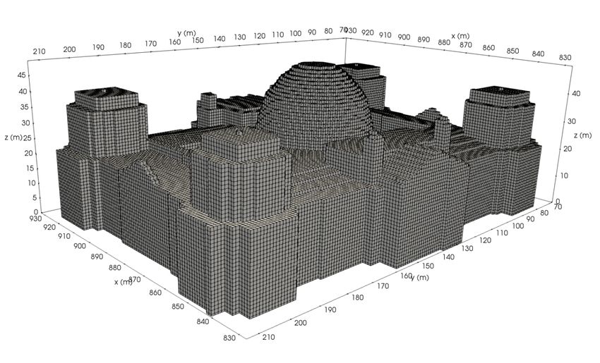
Table of Contents

City-descriptive input data for urban climate models: Model requirements, data sources and
challenges                                                                                    1
  Abstract                                                                                    3
  1)      Introduction                                                                        3
       1.1 Brief overview of urban atmospheric modelling                                      3
       1.2 Scale issues: mesoscale and microscale                                             4
       1.3 Coverage issues: from city-scale to global modelling                               5
       1.4 Fit for purpose                                                                    5
  2)      Land use and land cover classes                                                     7
       2.1 Description of the parameters and their relevance                                  7
       2.2 Methodologies to gather land cover data                                            9
         2.2.1. Remote sensing methods                                                        9
         2.2.2. From vector topographical databases and land registries                      10
         2.2.3. Data fusion                                                                  11
  3)        Morphological parameters                                                         11
       3.1 Description of the parameters and their relevance                                 11
       3.2 Links between morphological parameters                                            12
       3.3 Methodologies to gather morphological parameters                                  13
         3.3.1 Data from remote sensing                                                      13
         3.3.2 GIS treatment of 2.5D cadaster vector data of individual buildings            14
         3.3.4 Crowdsourcing or deep learning methods                                        18
  4)        Architectural parameters                                                         19
       4.1 Description of the parameters and their relevance                                 19
       4.2 Developing comprehensive architectural databases                                  20
       4.3 Methodologies to gather architectural information                                 21
         4.3.1 Identification of representative archetypes                                   21
         4.3.2 Remote sensing and image processing                                           22
         4.3.3 Crowdsourcing                                                                 23
  5)        Socio-economic data and building use                                             23
       5.1 Description of the parameters and their relevance                                 23
       5.2 Methodologies to gather uses, socio-economic and anthropogenic heat parameters    24
         5.2.1 From inventories                                                              24
         5.2.2 Crowdsourcing                                                                 26
  6)        Urban vegetation                                                                 27
       6.1 Description of the parameters and their relevance                                 27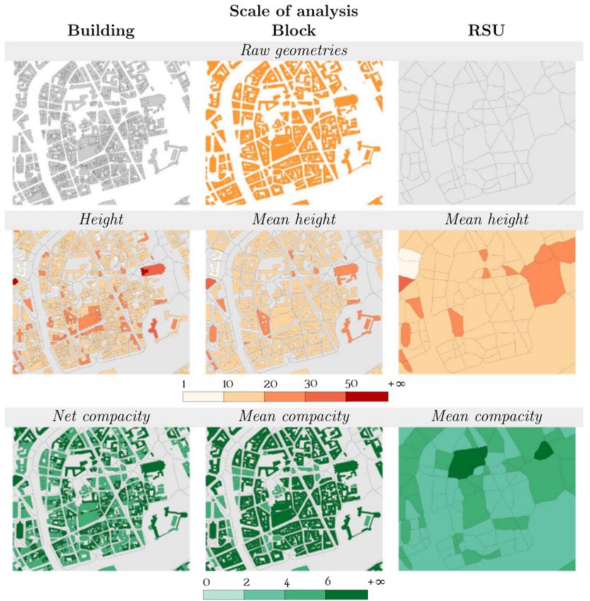
6.2 Methodologies to collect vegetation parameters at mesoscale                                        28
     6.3 Methodologies to collect vegetation parameters at microscale                                       29
  7) Discussion                                                                                             30
     7.1 Licensing issues                                                                                   30
     7.2 Cataloguing issues                                                                                 31
     7.3 Data quality                                                                                       31
     7.4 Open data                                                                                          31
     7.5 Research challenges for the next decade                                                            32
     7.6 From data of various origins to Urban Climate Services                                             33
  8 Conclusions                                                                                             33
  Appendix 1: Overview of several global land cover data sets with an urban description                     34
  Acknowledgements                                                                                          36
  References                                                                                                36

Abstract
Cities are particularly vulnerable to meteorological hazards because of the concentration of
population, goods, capital stock and infrastructure. Urban climate services require multi-disciplinary
and multi-sectorial approaches and new approaches in urban climate modelling. This paper classifies
the required urban input data for both mesoscale state-of-the-art Urban Canopy Models (UCMs) and
microscale Obstacle Resolving Models (ORM) into five categories and reviews the ways in which they
can be obtained. The first two categories are (1) land cover, and (2) building morphology. These govern
the main interactions between the city and the urban climate and the Urban Heat Island.
Interdependence between morphological parameters and UCM geometric hypotheses are discussed.
Building height, plan and wall area densities are recommended as the main input variables for UCMs,
whereas ORMs require 3D building data. Recently, three other categories of urban data became
relevant for finer urban studies and adaptation to climate change: (3) building design and architecture,
(4) building use, anthropogenic heat and socio-economic data, and (5) urban vegetation data. Several
methods for acquiring spatial information are reviewed, including remote sensing, geographic
information system (GIS) processing from administrative cadasters, expert knowledge and
crowdsourcing. Data availability, data harmonization, costs/efficiency trade-offs and future challenges
are then discussed.

1) Introduction
1.1 Brief overview of urban atmospheric modelling
Cities are particularly vulnerable to meteorological hazards because of the concentration of
population, goods, capital stock and infrastructure. In addition, they create their own urban micro-
climate because they have a strong influence on the local meteorology (Oke et al., 2017). For example,
heat waves, enhanced locally by the so-called 'Urban Heat Island' (UHI), can increase mortality rates
in cities (Fouillet et al., 2006; Tan et al., 2010). Large cities can also interact with local mesoscale flows,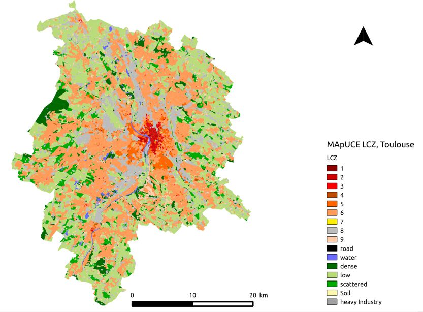
e.g., through intensification of the sea-breeze front due to thermal effects (Freitas et al., 2007), or, in
contrast, they can slow down breezes due to enhanced friction (von Glasow et al., 2013). Urban
climate also impacts the energy use of domestic heating and air conditioning (Ohashi et al., 2007;
Santamouris et al., 2015; Kohler et al., 2016), which, in turn, enhances the UHI due to the associated
heat release (de Munck et al., 2013; Wang et al., 2018). Thunderstorm activity can either be
concentrated in different parts of the city or be enhanced above or downstream of the city (Shepherd,
2005). In such a complex multi-dimensional and multi-objective decision environment, pertinent and
clear, decision-relevant information is indispensable for stakeholders, e.g., for fine-scale weather
forecasting in cities during sporting events (Joe et al., 2017) or for urban planning (Hidalgo et al., 2018).

Numerical modelling has become a useful tool for analyzing detailed urban meteorology and to design
urban climate services, e.g., to evaluate risks or benefits of urban planning or adaptation strategies.
To simulate urban climate, atmospheric models need to have an adequate representation of the
influence of the city on the exchanges with the atmosphere above. This is done using Urban Canopy
Models (UCMs). These UCMs (such as Masson, 2000; Kusaka et al., 2001; Martilli et al., 2002; Lee and
Park, 2008; Lemonsu et al., 2012; Schubert et al., 2012; Wouters et al., 2016) are surface schemes that
aim to represent the energy, water and momentum exchanges between the urban surface and the
atmosphere. They are often based on a simplified description of the 3D shape of the city, e.g., for
mesoscale modelling, the ‘urban canyon’ approximation is often used. Masson (2006) describes
several types of UCM according to their degree of complexity and realism, and Grimmond et al. (2010,
2011) further classify each physical component of these schemes, underlining the need for data to
describe the city. When going to the microscale, individual buildings are explicitly resolved by Obstacle
Resolving Models (ORMs) (Krayenhoff et al., 2015; Resler et al., 2017; Salim et al., 2018). These ORMs
create a high demand for detailed input data.

1.2 Scale issues: mesoscale and microscale
Mesoscale UCMs require suitable surface input data to provide reliable boundary conditions for
atmospheric models. The relevant and necessary spatial scale of these input data, however, strongly
depends on a) the atmospheric scale to be investigated, and b) the scale and level of detail of the UCM
applied. For mesoscale applications, this ranges from estimations of the roughness length as a first
order approximation of the friction due to urban canopies (Grimmond and Oke, 1999), to the more
advanced street canyon approach (e.g. Masson, 2006; Schubert et al., 2012), which requires the
determination of typical canyon parameters at the grid cell size of the atmospheric model. Note that
canyon here encompasses both impervious (e.g., roads, sidewalks, car parks, etc.) and pervious (e.g.,
vegetated) areas. For mesoscale models, this might be at the kilometer down to the hectometer scale.
However, for microscale models that operate at the meter scale, individual elements in the urban
canopy layer such as buildings, streets and trees are resolved explicitly. Today, urban microscale
models such as PALM/PALM-4U (Maronga et al., 2015, 2019a,b) are able to simulate city quarters at
a grid spacing of 1 m and entire cities at 10 m. It is obvious that such fine grid spacing requires the
input data to have a different level of detail. Moreover, many typical parameters that would normally
be derived must be replaced by the actual conditions of individual urban structures, such as specific
buildings or tree configurations in streets and parks. The building envelope is then no longer
represented by a simple street canyon but by individual surface elements that - as in reality - have
different insulation, window fraction, surface albedos, and which cast shadows on each other. The
high relevance of this information has been highlighted by Resler et al. (2017) in a systematic
sensitivity study of material parameters, where the sensitivity of the modelled surface temperature
reached up to 5°C with a variation in the surface albedo by ± 0.2. This paper illustrates that different
data acquisition strategies and data sources are required to fulfill the individual requirements of
numerical models.

1.3 Coverage issues: from city-scale to global modelling
Urban climate studies have been traditionally focused on the analysis of energy exchange and
turbulent processes using field campaigns or they have investigated the spatial distribution of the
temperature field from meteorological stations (Arnfield, 2003). Almost all of these studies have
focused on a specific site or on a given city where the physical description of the city was done locally.
This tendency has continued with the arrival of UCMs in the early 2000s, and weather forecasting
models that cover countrywide areas with UCMs (Seity et al., 2011) are now operational. There is now
more common use of atmospheric models for urban climate studies, and even recently, the
development of regional and global climate models (Oleson et al., 2011) with UCMs. This underlines
the necessity to have homogeneous descriptions and methods for producing urban parameters at a
fine resolution - typically one or a few urban blocks. This should be done in comparable ways for a set
of representative cities for scientific studies, and ideally worldwide.

The objective of this paper is to categorize the urban parameters needed for UCMs and then to discuss
their availability and acquisition. We start with a high-level categorization of 5 major types as follows:

    ●   Land use and land cover;
    ●   Morphological parameters;
    ●   Architectural parameters;
    ●   Socio-economic parameters and building use; and
    ●   Urban vegetation.

For each type, several possible ways to obtain spatially explicit parameters are presented and
discussed. The final section considers the availability and access to the data, the quality of such data
sets and the associated trade-offs between them.

1.4 Fit for purpose
The requirements for these urban parameters will depend on the purpose of each study. Before
detailed information is provided on how to obtain these parameters, it is important to stress that for
some applications, it may not be necessary to invest, either time or money, into the construction of
detailed maps of all parameters. The evaluation of the sensitivity of the model results on the accuracy
of the input urban parameters is out of the scope of this paper. However, some guidance may still be
given. Table 1 presents the type of parameters that are most crucial for several types of applications.
From a broad point of view, the higher the spatial resolution, the more detailed parameters are
required. However, the specific scope of a study, which could be, for example, the modelling of
pollutant emissions from domestic heating or the quantification of human thermal comfort, will have
a large influence on which input parameters are the most relevant.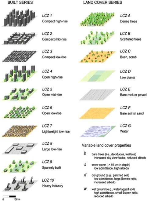
Land use/cover classes      Morphology      Architecture    Socio-economy &         Vegetation
                        Parameter     -     meso-scale:                                           uses                    description
                                      at neighborhood scale       incl. height,
                                      (e.g. LCZ)                  building &                                              (Type, LAI,…)
                                                                  (im)pervious
Purpose                               -     micro-scale:          fractions…
                                      urban elemental objects
                                      (e.g. buildings, roads)
At meso-scale
1km-res NWP & climate models          x (at neighborhood scale)
100m res NWP                          x                           x

Forcing of AQ models                  x
Forcing of & interactive emissions    x                           x               x               x
of buildings for AQ models
At micro-scale
1m-res Building resolving modelling   x (urban objects)           x                                                       Leaf Area Density
Radiative effects, shadows            x                           x               Albedo (incl.                           Leaf Area Density
                                                                                  Windows)
Flow modification                     x                           x                                                       Leaf Area Density
Development of parameterizations      x                           x               Possibly        Possibly                Possibly
                                                                                  (e.g. energy    (e.g. traffic induced   (e.g. pollutants
for urban climate processes                                                       balance)        turbulence)             dispersion)
At both micro and meso-scales
Outdoor heat-stress quantification    x                           x               Albedo (incl.                           x
                                                                                  Windows)
Indoor heat-stress and Energy         x                           x               x               x
consumption quantification
CO2 fluxes in urban areas             x                           x               x               x                       x
Urban hydrology modelling             x                           Coverage                                                x
                                                                  fractions

          Table 1 : Parameters needed in order of priority depending on the purpose.

          In current meso and microscale model applications, it is possible, and even common, to only use a
          map of land use/land cover to completely initialize all the other parameters. This is done through look-
          up tables that assign uniform values to each morphological (e.g., building height, building density) or
          other parameter depending on the land cover type (e.g., higher and denser buildings in “dense urban”
          compared to “suburban”). This is defined as the ‘indirect method’ in Figure 1. Numerical Weather
          Prediction (NWP) and its direct application to provide meteorological forcing to Air Quality (AQ)
          models applied at a kilometric scale typically relies on such look-up tables. This assumes that at a
          spatial scale of 1 km x 1km, details on the urban structure are of minor relevance for weather
          forecasting and air quality modelling. However, to fully benefit from an increased horizontal resolution
          (e.g. 100 m) of NWP and AQ models, and to be able to simulate fine-scale impacts (see Table 1), it is
          recommended that a fine scale description of the urban parameters is provided, with a priority to be
          given to the morphological parameters. This requires employing ‘direct methods’ using ancillary data
          (e.g., remote sensing or building cadasters) to compute these parameters. A summary of these direct
          methods is provided in Figure 1, and they are (briefly) presented throughout this article for each of
          the 5 types of parameters.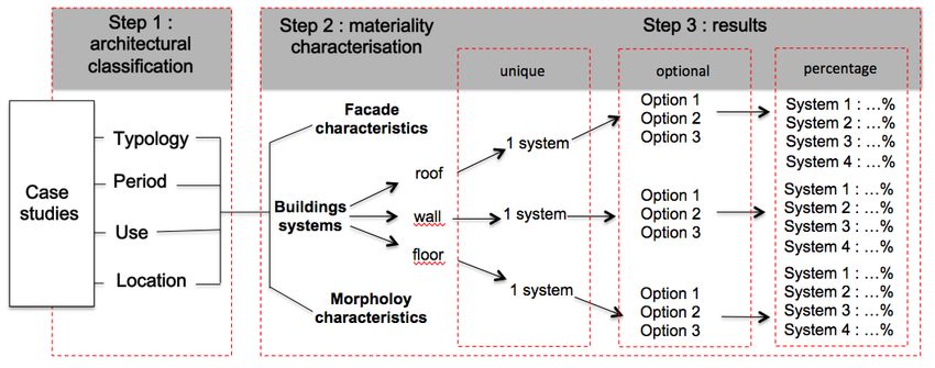
Land cover / land use classes (§2)
          Build up and impervious classes
                    (micro-scale)                                      Vegetation and           Methods:
                                                    Water
                                                                         soil classes           - Remote-sensing
                    Urban classes
                (neighborhood scale)                                                            - Fromland registries

                  Morphology (§3)                       Architecture (§4)               Socio-economics & building use (§5)
                          Methods:
                                                             Building type                Building use      Population density,
       road, pervious,
                                                                                                            Occupancy & uses
       impervious and     - Remote-sensing
           building       - Fromland registries              Architecture,                Methods:
          fractions                                           Materials…                  - Frominventoriesand census
                                                                                          - Crowdsourcing
                          - Radar remotesensing
          Mesoscale       - Stereo photogrametry      Methods:
           Buildings’     - From2.5Dbuilding                                               Vegetation characteristics (§6)
          aggregated        databases                 - expertise/literatureon
         information      - Deep learning from          construction practices          Methods:
                            photographs               - Imageprocessing                 - Remote-sensing (Lidar, NDVI, …)
                                                      - crowdsourcing                   - Fromland registries
                                                                                        - In-situ observations
         Microscale
         3D building      - Lidar Remote-sensing
           shape          - 3Dbuilding databases
                                                            Legend on Methods to provide the parameters:
                                                            Indirect method from another parameter:
                                                            Direct method from ancillary source of data: - italic text

Figure 1: Overview of the methods to provide the parameters

2) Land use and land cover classes
2.1 Description of the parameters and their relevance
The physical and biophysical cover of the Earth strongly modifies the momentum, energy and water
fluxes of the atmosphere above. The sensible heat flux is generally enhanced above impervious
surfaces, while evapotranspiration by soil and plants will favor latent heat fluxes. Drastic spatial
heterogeneity in land use and hence on land cover, like that which happens in coastal cities in sea
breeze conditions, can significantly influence the entire boundary layer above a city when compared
to a continental city. Therefore, the mapping of urban, vegetation and water cover is essential and
can be further refined, depending on the model requirements. The class ‘water’ can, for example, be
separated into sea, rivers, lakes, and ponds. Vegetation is often separated into high and low
vegetation (see section 6 for further discussion).

Currently, there is no global data set on the urban tissue that can directly provide the most relevant
parameters for UCMs (e.g., plan area, building density, building height, etc.). Instead, such parameters
are derived from available land cover products using the relevant classes and a set of heuristics. There
are two common ways to estimate the required parameters. The first option is to provide a map of
each required parameter to the model. This approach is described in sections 3 to 6. However, it is
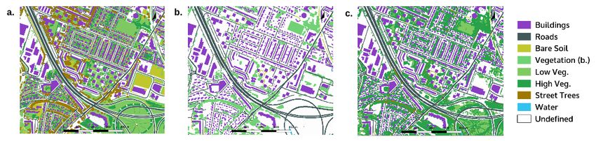
generally impossible to have such a fine description for all of the UCM parameters for any given city
of investigation. Therefore, the second option must be used for parameters that are unavailable,
which is to employ land cover maps. Existing land cover products, e.g., produced automatically from
remote sensing imagery, are of crucial interest since they usually identify urban areas. However, they
can also be used to estimate all the other parameters related to morphology, architecture, the social
and economic environment and vegetation, by using a lookup table, particularly when other sources
of information are lacking (or not used).

At meso-scale, the absolute minimum information is to have at least one class called “urban” within
the land cover map, and to assign uniform values to this class for all urban model parameters across
the globe. Most databases used in atmospheric models, even recent ones, have only one urban class.
Depending on the model requirements and the available data, the urban class can be refined in several
ways. For example, it can be separated into different urban densities, which commonly refers to the
density of the buildings although population density would be an alternative method. These classes
typically use either the land use or land cover (and often both) to describe the city at the neighborhood
scale.

Examples of global land cover maps with one single urban class are the satellite-based GlobCover (300
m, one class ‘artificial surfaces and associated areas’; Arino et al., 2008), MODIS Land Cover (500 m,
one class ‘urban and built-up land’; Friedl et al., 2010), the ESA-CCI (300 m; one class ‘urban areas’;
Bontemps et al., 2013) and GlobeLand30 (30 m, one class ‘artificial surfaces’; Chen et al., 2015).
Several regional and global initiatives have been undertaken to gather a more detailed description of
the urban tissue. An example is the Global Human Settlement Layer (GHSL) LABEL product (38 m
resolution; Pesaresi et al., 2013, 2016). This data set distinguishes roads, built-up areas with different
densities (very light/light/medium/strong) and for the strongly built-up areas, the building height (low
rise/medium rise/high rise/very high rise). Congalton et al. (2014) and Grekousis et al. (2015) review
a large number of global and regional land cover products. A (non-exhaustive) overview of global and
regional land cover data sets that are suitable for urban climate modelling is provided in Appendix 1.

The deployment of the Local Climate Zone (LCZ) typology (Stewart and Oke, 2012, Figure 2)
standardizes the way that UCM parameters are described. This typology aims to characterize the
urban tissue and induce urban climate heterogeneity at the neighborhood scale (typically ≥ 1 km2).
LCZs represent urban areas that are relatively homogeneous in their type of urbanization. They
represent either the rural landscape (in seven classes: dense or scattered trees, bushes, low plants,
bare soil, bare rock, water) or the urban landscape, more specifically, in ten classes (compact or open
high-rise buildings, compact or open mid-rise buildings, compact, open or sparse low-rise buildings,
large low-rise buildings, heavy industry, lightweight low-rise buildings). LCZs are provided with ranges
of values for a few UCM parameters, which are the sky view factor, the aspect ratio, the mean building
height, the terrain roughness class, the building, pervious and impervious surface fractions, the overall
thermal admittance and albedo, and the anthropogenic heat flux. This approach aims to be ‘universal’,
i.e., with limited cultural bias, which means that it can be applied to cities worldwide. LCZs are
intended to represent areas that have, independently of other geographic or topographic factors, a
homogeneous local thermal climate. A few experimental campaigns, such as Houet and Pigeon (2011)
using fieldwork, air temperature measurements and surface temperature satellite images, or Leconte
et al. (2017) with an instrumented car, have confirmed that this assumption is correct. For ORMs,
however, the above data sets and approaches are not sufficient as the urban canopy must be
described explicitly.

At micro-scale, much finer spatial details are necessary for describing the urban surface. Contrary to
the land use and land cover classes that represent the city at the neighborhood scale, here it is
necessary to describe the elemental objects of the city individually. Another approach is to describe
the urban land cover by its components, thus mapping urban objects such as buildings, paved surfaces
(roads, etc.) and meadows, which is a typical approach for ORMs.

Figure 2: LCZ classification scheme. Left: LCZ description (source: Stewart and Oke 2012); right: vector
based LCZ map of Toulouse, France at urban block scale produced using a building registry.

2.2 Methodologies to gather land cover data

2.2.1. Remote sensing methods

Remote sensing is a convenient tool for land cover mapping. It can cover large areas at once, allow
comparable mapping across different cities, and the data sets can be updated quite easily. However,
several aspects need to be considered when selecting a suitable sensor. The spatial resolution and the
classification scheme need to be defined. When more classes need to be considered, then the remote
sensing data will need more spectral and spatial detail. A suitable classification scheme for remote
sensing applications for urban climate is the Vegetation, Impervious and Soil (V-I-S) approach by Ridd
(1995), which also addresses the mixtures of land cover within one pixel. Often the impervious surface
is separated into a high and a low albedo class (Lu and Weng, 2006), especially at higher spatial
resolutions (Yang and He, 2017). The V-I-S approach has, for example, been applied to UHI mapping
and surface temperature studies (e.g. Zhang et al., 2015; Wang et al., 2016).

With higher spatial and spectral resolution, more classes can be distinguished, such as buildings and
pavements (e.g. Thomas et al., 2003) up to material mapping with high resolution hyperspectral
remote sensing data (Heldens et al., 2017). Once the classification scheme has been determined, a
suitable sensor can be selected. For spatial resolutions coarser than 10 m, many satellite systems are
available. Depending on the sensor, the data can often be obtained for free. Spatial resolutions of less
than 10 m require high resolution imagery, which is often not freely available. In addition to satellite
data, airborne sensors can also be used. Based on the classification scheme and the remote sensing
data, the classification method is then selected. Generally, supervised and unsupervised methods are
available. An overview of land cover mapping techniques is addressed by Lu and Weng (2007) or Ban
et al. (2015).

For high resolution data, object-based classification techniques can be used (Ma et al., 2017).
Considerable research efforts are being directed towards developing and improving machine learning
techniques, and they are especially promising for complex classification tasks (Maxwell et al., 2018).

A land cover classification approach that has been developed specifically for urban climate
applications is the World Urban Database and Access Portal Tools (WUDAPT) project. This is an
initiative started by the community of urban climatologists (Bechtel et al., 2015; Ching et al., 2018),
which proposes a common methodology for producing LCZ raster maps using supervised classification
of satellite images. Some large areas have already been covered at a 100 m resolution, such as China
and Europe.

2.2.2. From vector topographical databases and land registries

In addition to remotely sensed imagery, vector-formatted information about the urban built
environment and human activities in cities is a useful resource for mapping land cover (and to derive
parameters for UCMs). Typical sources of such vector data are local, national or European public
agencies (e.g., planning agencies, mapping or statistical institutes, land and property registries,
Eurogeographics, which is a consortium of national mapping agencies producing European products),
private companies (e.g., real estate brokers, environmental services companies, transportation
consultants), international organizations (e.g., the European Environment Agency, the European
Commission’s EUROSTAT agency and the thematic data banks of the World Bank, International
Monetary Fund, or the United Nations), and crowdsourced initiatives such as OpenStreetMap1 (OSM).
OSM is an initiative in which volunteers contribute to a global map of the world (Mooney and
Minghini, 2017).

One method to extract land use information from vector data sets is to combine cadaster plans of land
plots and buildings with the information that is registered about these geographical entities in, e.g.,
taxation, planning permits, or ownership records. GIS (or AutoCad) software can be used to develop
combined data sets that represent urban land patches and built structures in very high spatial
resolution together with detailed information about their uses, which can then be transformed into
land use maps. Another method is to use the vector polygons of building footprints and other man-
made structures contained in the aforementioned data sets to “tag” those pixels in existing land cover
maps as “urban” when these footprints and structures are encountered (see e.g. Jantz et al., 2004).
This provides the possibility of creating more detailed urban classes since building footprints often
contain information on their type and use. Similar to the above, a third method is to access spatial
data services, e.g. the OSM query service or national portals to request semantic information about
particular coordinate points or polygons. The semantic information can include the type of human
activity reported for a specific structure, e.g., recreation, shopping, dining, etc., or the general
category to which a structure is classified, e.g., residential, commercial, government, etc. This
approach can be used to develop land use maps or enhance existing land cover maps (Olbricht, 2015;
Boeing, 2017). Such methods using administrative cadasters have been used to map LCZs by Kotharkar
and Bagade (2018) for Nagpur in India, Geletič and Lehnert (2016) for three cities in the Czech
Republic, by Zheng et al. (2018) in Hong Kong and for French cities by Hidalgo et al. (2019) (Figure 2).
UCMs with a grid resolution finer than 25 m require more detailed land cover/land use data. In
Germany there are area-wide cadasters available as ALKIS (Official Real Estate Cadastre) and ATKIS

1   http://www.openstreetmap.org/
(Official Topographic Information System), which provide land cover and land use data at different
scales. These systems are updated and validated every year. Comparable products exist in every
European country. The INSPIRE directive aims to reuse such national data for monitoring European
environmental activities and to design European policies in order to have more consistency between
the local and European levels. To achieve this goal, a federated workflow for such content has been
designed, and every country must publish data produced by legally mandated organizations through
web services according to interoperable specifications at the European level. OSM might also be used
as a data source at this high resolution although the quality differs largely across different areas.
However, the quality is sufficient as an input to ORMs and UCMs in densely populated areas, especially
with regard to the building footprints.

2.2.3. Data fusion

The data required on land cover or land use can often not be represented with sufficient accuracy by
one of the aforementioned data sets alone. A good alternative is to combine multiple data sets to
improve the resulting information layer. Such a data fusion approach can, for example, rely on signal
processing techniques to merge different spectral signatures to yield materials information, on
photogrammetric techniques to merge data with different angles to obtain 3D information, or on
advanced GIS operations to combine different spatial formats (i.e., raster, vector and tables). For
example, GIS information can be combined with remotely sensed information as proxies for
parameters. This approach can be used to derive highly detailed land use and building use information
by associating temporal, spatial and spectral information patterns to particular human activities, often
with the help of deep learning algorithms (Ebert et al., 2009; Ghaffarian et al., 2018). It is very
important, however, to have good information about the quality of each data set, as they might
contain the same information with different qualities or spatial resolutions.

3) Morphological parameters
3.1 Description of the parameters and their relevance
Morphological parameters allow the 3D aspect of the city to be described, and they influence the
momentum as well as radiative exchange, with shadowing and multiple reflections between buildings,
leading to infrared radiation trapping (especially during nighttime). Furthermore, the 3D character of
buildings increases the volume covered by solid materials and the amount of surface area that is in
direct contact with the atmosphere. The 3D character of cities, and the thermal properties of
construction materials, favor the storage of heat inside the urban canopy. Both aspects are the main
physical reasons leading to the development of the nocturnal UHI. At the microscale, these processes
are simulated by the explicit interactions between individual buildings. In order to represent them in
ORMs, detailed information on the 2D and 3D urban structure is needed at a decameter to meter
scale. The relevant morphological parameters here are the 3D building configuration, i.e., the
information regarding which grid volumes are covered by built-up structures, including thoroughfares
and bridges, and 2D maps of the surface configuration regarding impervious (roads, footways, parking
lots, etc.) and pervious surfaces (water, vegetation, soil). At the mesoscale, these parameters are
statistically aggregated into indicator values. Many indicators exist, some of which may be retrieved
by combination with others. For mesoscale UCMs, typical morphological parameters that should be
produced are described in Table 2.
Parameters                     Comments

 building fraction λp           Surface of buildings Sbld, seen from above divided by the
                                horizontal surface of the urban area under consideration, Shor

 pervious and road fraction     Idem, for pervious and road/impervious surfaces

 wall density λw                Ratio between the surface of walls in contact with the
                                atmosphere, Sw, and the horizontal urban surface, λw=Sw/Shor

 mean building height, h        This is, along with λp, the key parameter needed by all UCMs.

 σh                             Standard deviation of the building height

 roughness length z0            While this is fundamentally an aerodynamic parameter describing
                                the air flow above a surface, it is classically estimated from the
                                structure of the surface below. There are many ways to estimate
                                the roughness length mathematically in cities (Grimmond and
                                Oke, 1999). Strictly speaking, the roughness length is only
                                applicable for uniform homogeneous surfaces, but due to lack of
                                alternatives, it is often also applied to heterogeneous surfaces
                                and buildings.

 h/w and Ψ                      Canyon aspect ratio (building height divided by the canyon width,
                                h/w) and sky view factor Ψ, which describes the compactness of
                                the city.

 Frontal area density, λf       λf is the surface of walls facing the wind normalized by the
                                horizontal surface. λf < λw. It depends on the wind direction.

Table 2: Typical morphological parameters used by UCMs

In multi-layer models with intersecting atmospheric layers (Martilli et al., 2002; Hamdi and Masson,
2008), the friction is simulated using a drag coefficient approach. For this purpose, λf which describes
the vertical arrangement between buildings, is often coupled with λp, because together they represent
the nature of the breathability between the canopy and the atmosphere.

The canyon aspect ratio (h/w) and sky view factor Ψ describe the ability of the city to trap the
radiation. A large h/w (small Ψ) ratio favors the storage heat flux while a low sky view factor reduces
longwave radiation loss at night, but also reduces shortwave gain during the day.
3.2 Links between morphological parameters
In reality, the variety in the urban tissue and the arrangement between buildings of diverse shapes
can lead to various combinations of parameters for a given area (either a grid mesh of the model, or
an LCZ or urban block). In other words, all of these parameters can be mapped independently.
However, when using morphological parameters in mesoscale UCMs, they assume a simplified
geometry. This implies: (1) that the UCMs cannot simulate all of the internal variability of the urban
tissue, and (2) that these morphological parameters are no longer independent. This means that one
cannot specify many of them independently using fine scale data without violating the physics and
energy conservation within the UCM. This is why model developers have to identify: (1) which
parameters are absolutely necessary; (2) which can be deduced from others (but could be estimated
independently if the data are available); and, (3) which must be, in order to conserve the consistency
of the UCM, deduced from others.
Parameters entering in momentum flux parameterizations are generally in the second category.
Building heights, or λf and λp, can be used to define the roughness length (Grimmond and Oke, 1999)
and drag coefficients (Santiago and Martilli, 2010). All parameters can also be used freely for
diagnostic purposes, e.g. fine-scale maps of Ψ can be used for human comfort evaluation at several
places within the canyon (or more generally the city), even if they are not used directly as an input to
the UCM for the calculation of the surface energy balance. However, when energy balances of
individual surfaces (such as roofs, walls, roads, vegetation) are considered, some parameters can no
longer be independently specified from the others. Most UCMs are based on the canyon hypothesis,
which assumes that there is an infinitely long street canyon, bordered by two walls of identical height.
This produces some relationships between morphological parameters that cannot be considered
independently any more. Energy conservation is governed by the amount of each surface in contact
with the atmosphere, and radiative exchanges by how the surfaces ‘see’ each other. In the infinite
canyon geometry, this implies, for the normalized wall surface λw, that the canyon aspect ratio h/w,
the plan area density (or building fraction) λp, and the sky view factor in the middle of the street Ψ
(from Noilhan, 1981) can be expressed as follows:
λw = 2 (1-λp) h/w (1)
Ψ = [ (h/w)2 + 1 ]1/2 – h/w (2)
This means that when maps of λp, λw, Ψ and h/w are available, only two of them should be used for
the calculation of the UCM energy balance. Therefore, the two recomputed parameters would not be
coherent with the actual city data. Hogan (2018) has explored another geometric hypothesis based
on an exponential distribution of road widths, and has shown that the induced relationships between
morphological parameters can also be computed using only λp, λw and the building height.
Given (1) the difficulty in defining what a canyon width (w) is for a heterogeneous real urban tissue,
or where to define the middle of the road required to calculate Ψ, and (2) the importance of the
quantity of the surfaces in contact with the atmosphere for energy exchange, we strongly recommend
using the following as primary parameters: building height, the building fraction, λp, which is classical,
and the normalized wall surface, λw, even though the latter parameter is not generally considered as
an independent input parameter in UCMs.3.3 Methodologies to gather morphological parameters 3.3.1 Data from remote sensing Due to the capability of cost-efficient large-area data collection, remote sensing has become a key source for describing the 3D structure of the built environment. The most commonly used baseline product for urban structural analyses derived with remote sensing technologies is the digital surface model (DSM). A DSM provides a detailed picture of the terrain surface along with all other vertical features such as buildings and infrastructure elements or trees and hedgerows. To more effectively describe and analyze vertical objects not related to the terrain topography (e.g., buildings), a normalized DSM (nDSM) is usually calculated by subtracting the modelled terrain height (digital terrain model) from the DSM (Weidner and Förstner, 1995; Reinartz et al., 2017). The traditional technique for DSM/nDSM generation and subsequent analysis of the urban morphology is photogrammetric processing of optical stereo imagery from sensors mounted on airplanes (Fradkin et al., 1999; Hirschmüller et al., 2005) or from high and very-high resolution satellite data (Toutin, 2006; Eckert and Hollands, 2010; Sirmacek et al., 2012; Aguilar et al., 2014). Recently, unmanned aerial vehicles (UAVs) have increasingly been deployed to measure the 3D urban morphology. Gevaert et al. (2017) describe how point-cloud and image-based morphologic features derived from UAV data can be used to classify specific built-up structures related to informal settlements. Esch et al. (2018a) describe new perspectives for surveying local urban morphology arising from the utilization of drones, UAVs or High-Altitude Pseudo Satellites (HAPS). An established alternative to stereo photogrammetry is the analysis of point clouds from airborne light detection and ranging (LiDAR). LiDAR systems send laser pulses towards the ground whereas the runtime length can be used to generate precise DSMs (Vosselman and Maas, 2010). Usually, LiDARs collect a cloud of 4-50 points per m² and thereby allow for a detailed characterization of the small- scale urban morphology (Jutzi and Stilla, 2003; Goodwin et al., 2009; Yan et al., 2015). Bonczak and Kontokosta (2019) demonstrate the application of point-based voxelization techniques to extract design parameters in complex urban environments in unprecedented spatial detail. Moreover, synthetic aperture radar (SAR) technology can be employed to generate DSMs for urban areas by means of spaceborne SAR interferometry (InSAR) or SAR tomography (Fornaro and Serafino, 2006; Frey et al., 2014; Marconcini et al., 2014; Geiß et al., 2015; Zhu et al., 2016). However, regarding InSAR, the spatial resolution of the resulting DSMs is usually lower than the products derived from optical satellite systems, whereas SAR tomography is still a rather experimental method due to the massive satellite data requirements. The Urban Atlas land cover/land use product from Copernicus has recently added building height data for the capital cities of EU countries. Although covering only a large (700) but still limited number of cities, this can provide data for testing/validation. This information is also available in the INSPIRE data and in the European Location Service. 3.3.2 GIS treatment of 2.5D cadaster vector data of individual buildings GIS software is often used to compute morphological indicators such as the density of buildings, the mean building height, the compactness ratio, the sky view factor, etc. These indicators are applied to study and monitor the urban structure at different geographic scales (e.g., urban parcels or districts). Techniques are based on spatial analysis chains that use geometric data models (also called vector data). Urban features are represented by a set of polygons (e.g., buildings), lines (e.g., roads) or points
(e.g., elevation) grouped in GIS layers restricted to a 2.5D dimension. A vector data model offers
several advantages for urban climate studies:

    ●   It is able to store many parameters in one layer. For example, if a building is represented by a
        set of polygons, additional attributes such as height, age, floor area and wall material can be
        specified to describe it.
    ●   It allows an accurate representation of urban geometry allowing urban climate models to
        operate on a very fine scale (e.g. 1 m). Berghauser Pont and Haupt (2005) define a building
        block as an aggregation of buildings that are in contact. The building block concept allows
        architectural patterns in the urban fabric (mid-rise compact building, closed blocks, etc.) to be
        retrieved. This scale is particularly useful for studies dealing with the interaction of urban
        climate and building energy demand (Bouyer et al., 2011).

Most GIS approaches use a regular vector grid to represent the urban space and compute the
morphological indicators inside the cells (Lindberg, 2007). Ching et al. (2009) compiled data on
buildings and urban vegetation (mainly via airborne LiDAR detection), anthropogenic heat release due
to buildings, traffic and human metabolism (via a top-down approach combining energy consumption
data and the regional climatic conditions), as well as day- and night-time population density (via
census data) for approximately 130 US cities.

Although a regular grid may be suitable for populating a climate model, it also represents an abstract
feature that does not conform to real parcels or urban forms, which tend to have irregular shapes and
their own distinct spatial boundaries that stem from socioeconomic processes. Cities are often
characterized by complex spatial assemblages that are smoothed out when using regular grids; the
challenge is to utilize a representation of space that fuses both options and is therefore suitable for
the representation and modelling of both physical and socioeconomic processes.

Dealing with a detailed mapping of urban areas that describe their morphology and spatial
relationships is an old but still very relevant issue. Barnsley and Barr (1997) proposed a GIS graph
model to perform a spatial classification of a geographically referenced digital urban map. Steiniger
(2006) extended their set of morphologic properties to classify urban structures for mapping
purposes. Bocher et al. (2018) describe a GIS processing chain to compute a set of morphological
indicators based on 2.5D vector data available for the French territory. 64 indicators were calculated
at three scales: individual buildings, blocks of buildings and a specific unit area called a Reference
Spatial Unit (Figure 3). These indicators are combined with socioeconomic data to categorize the
urban fabric.
Figure 3. Maps for the three geographical scales (individual buildings, blocks of buildings and Reference Spatial Units) used to compute the morphological indicators. Source: Bocher et al (2018). Samsonov et al. (2015) presented an advanced GIS technique to extract urban canyons from vector databases. The authors used a constrained Delaunay triangulation to delineate a hierarchy of the canyons based on the geometric properties of the triangles and their spatial relation with urban features, buildings and the street network. The morphological properties of the canyons are then combined with derived indicators (such as sky view factor and frontal area index) to feed the URB_MOS meteorological model. An application is discussed for the city of Moscow to model the spatial distribution of temperature and wind. 3.3.3 3D building data and CityGML for microscale modelling The CityGML standard2, developed by the Open Geospatial Consortium (OGC), defines three- dimensional geometry, topology, appearance and semantics of all relevant topographic urban objects at multiple well-defined level of details (LOD), ranging from simplified bounding boxes (LOD1: constant building height, LOD2: with roof shape) to explicit details like doors (LOD3) or indoor design (LOD4) (Gröger and Plümer, 2012). Because they represent the explicit form of buildings, they benefit ORMs 2 https://www.opengeospatial.org/standards/citygml
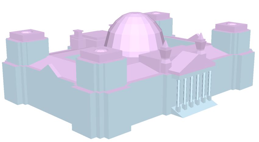
more than UCMs in being able to use this finer scale data (e.g., LOD2, cf Figure 4). CityGML is very
generic and does not only include all 3D objects of interest to ORMs, like buildings, trees, bridges,
tunnels or even park benches, but it contains also basic classes such as relief, water bodies, roads or
land use. Most available CityGML models have been automatically generated from a fusion of LiDAR
and catastral data. Important landmarks are often manually added at a higher level of detail. Creation
and improvement of CityGML data sets is an ongoing project for many municipalities. Germany, for
example, plans to offer a comprehensive LOD2 building model by 2019 and to amend it with bridges
and tunnels by 2020. The detailed CityGML data can then be rasterized and aggregated to the
resolution and requirements of the ORM model. For ORMs at the meter resolution, information about
textures can also be mined using machine learning approaches, e.g., to extract information like
building materials and window or vegetation fractions for single facades.

As an example of the processing of CityGML data to represent buildings in a microscale simulation of
Berlin at a grid spacing of 1 m, Figure 4 shows the original LOD2 CityGML while Figure 5 is the voxeled
building configuration of the Reichstag building in Berlin, Germany.

German municipalities and/or federal states usually order laser scan data collections to generate their
high-resolution 3D city models. Such data sets are updated every 5 years. After data collection,
georeferencing and further processing lead to a 3-dimensional point cloud, which is the product of
the first processing step. The subsequent categorization into different object types like buildings or
vegetation is either already done by the data supplier or must be done by the end user. If such a
categorization is missing, a common method to obtain the different object types is the intersection of
the height information with land cover data, e.g., building footprints or by a classified Normalized
Difference Vegetation Index (NDVI) layer, which divides the whole domain into pervious and non-
pervious areas to categorize the point cloud. Further classification steps may be necessary to obtain
the required input data structures for the respective ORM.

Figure 4: Original LOD2 3D CityGML representation of the German Reichstag Building, Berlin.
Figure 5: 3D visualization of a processed and rasterized CityGML representation of the Reichstag
building in Berlin, Germany, at a grid spacing of 1 m.

The design of 3D data products at the national level has been considered for several years now (Stoter
et al., 2015). Optical imagery with different angles is used to generate elevation models with
photogrammetric technologies. This technique can be applied to airborne imagery using several
images from the same flight but it can also be improved with UAVs or street imagery. LiDAR offers a
higher geometric accuracy but a smaller coverage. In some countries, nationwide LiDAR products are
available (as over the USA, Ching et al., 2009). For some areas, simplified 3D databases can be built
automatically out of existing topographic databases based on height attributes. For example, Brasebin
et al. (2012) showed that the French national topographic product implementing INSPIRE can be used
to analyze sky view factor when aggregated results are needed. The buildings are captured at the
gutter level and have metric information about the height of the building.

3.3.4 Crowdsourcing or deep learning methods

Data on building heights can also be crowdsourced directly (Over et al., 2010; Fan and Zipf, 2016)
through OSM. OSM has an agreed set of tags for 3D building models including ‘height’ for height of
the building in meters and ‘levels‘ for the number of floors. Although this information is not often
added to buildings footprints in OSM, there are some demo cities with this information that can be
visualized via the OSM Wiki3, but building height is often missing (Lao et al., 2018). They report that
less than 3% of the buildings globally have a height value and less than 4% have a level value. For the
city of Paris, the values are 0.1% and 51.2%, respectively.

It would be possible to use crowdsourcing to manually extract building height or the number of floors
from photographs in Google Street View, Mapillary or from other geo-tagged photo repositories such

3   https://wiki.openstreetmap.org/wiki/Simple_3D_buildings
as Flickr. This would involve building a bespoke application for this data collection but it could provide
a sample of building heights across a city that would be adequate enough for urban climate modelling
purposes. Similarly, an application could be built for collecting this type of data on the ground.

Biljecki et al. (2017) developed a model to predict the building height based on parameters from the
building cadaster, the geometry of the buildings from OSM and information from the census. Exploring
the combination of different parameters, the mean absolute error of predicted building height varied
from 0.8 to 3.1 m. Photograph or image analysis by deep learning is also being developed to extract
some morphological parameters. For example, Liang et al. (2017), Gong et al (2018) and Middel et al
(2018, 2019) showed that it is possible to analyze Google Street View photographs to map the sky
view factor. Zhang et al. (2019) developed a procedural model using neural networks to produce a 3D
model of buildings in cities from segmented satellite images, OSM street information, population
density and terrain elevation.

4) Architectural parameters
4.1 Description of the parameters and their relevance
Architectural parameters describe the way that buildings are constructed. The choice of building
materials and structure modify the heat conduction, and the roof cover and walls affect the radiative
exchange with the atmosphere. Hence, they can strongly modify the UHI. Many adaptation strategies
are based on modifications of these characteristics because they are relatively easy to implement,
since this occurs at building scale. An example are white roofs or walls, which reflect the solar energy
towards the sky (see Santamouris, 2014 for a review). Many traditional villages around the
Mediterranean Sea are built this way. Another aspect relates to wall insulation, when present;
depending if the insulation is on the inside or the outside, the total energy stored during daytime in
the building fabric will be different, and hence so will the UHI. Architectural parameters are building
materials, depth, thermal conductivity, and heat capacity (or thermal diffusivity) of all walls or for each
layer of wall (e.g., for the layer of structural material and for the insulation layer inside or outside),
and of the roofs. A description of the intermediate floors is required if a Building Energy Module (BEM,
e.g. Salamanca et al., 2009; Pigeon et al., 2014) is included in the UCM, as is the case, for example, for
BEP (Building Energy Performance) and TEB (Town Energy Balance) models. The presence of windows
is also important, as it modifies the internal energy balance of the buildings and the subsequent
anthropogenic heat emissions due to domestic heating or air-conditioning. Furthermore, windows
have different thermal and radiative properties than walls. In particular, the knowledge of both the
location and the window fraction per surface element (or per square meter) become important for
microscale simulations where the spatial variations of windows can be explicitly represented (Resler
et al., 2017). Also, green roofs and facades are a known strategy for the cooling of cities and should
thus be taken into account in modelling studies. This is not only important at the urban scale, but
particularly at the microscale, as green elements are altering the thermodynamic conditions,
especially in the vicinity of their location.

To summarize, the most important parameters include:

    ●   albedo and emissivity of walls and roofs;
    ●   thermal properties (thermal conductivity and heat capacity) and thickness of the layers of
        materials constituting the roofs and walls;
    ●   the fraction of windows on the external facades;
    ●   the thermal characteristics of the windows;
● the presence of shelters on windows
4.2 Developing comprehensive architectural databases
There exists for no large city an exhaustive database on building architectural practices or building
material characteristics at the scale of the building. Even with the increasing use of Building
Information Modelling (BIM), such information is, at best, limited to a very small part of buildings in a
city, which are mostly recently constructed large buildings. Due to the specific lack of spatial data
about architectural structures at the city scale, how can such parameters be defined? The main
problem is that all of these parameters depend on the materials used to construct the buildings, and
this varies considerably across time and space. Almost no generic information exists about these
architectural features and certainly not globally. Even at the local scale, the only comprehensive way
to gather data on building materials is limited to roof material identification using hyper-spectral
remote-sensing (Heiden et al., 2007). Architectural knowledge is mostly available at the building scale,
but not extensively. The issue arises of how to upscale such sparse information. Some attempts have
been made to derive surface parameters like wall albedo and emissivity as well as window fractions
by manual observations within case studies (Resler et al., 2017).
As databases of the architectural parameters needed by UCMs and ORMs are not available, an
approximate approach is possible, i.e., the development of comprehensive architectural databases.
The objective is to describe, for several archetypes of buildings, their typical architectural
characteristics. For example, the material of the main structural wall is documented. To link this
information to the models, the thermal characteristics of these materials are recorded. While these
parameters still only represent an educated guess, they allow the variability in building architectural
characteristics to be taken into account. Jackson et al. (2010) have described the thermal and radiative
properties of buildings for 4 building types in 33 regions in the world (defined by socio-economics,
architectural practices and climate). Tornay et al. (2017), using an architect’s expertise approach, have
defined building archetypes in each of the 95 administrative regions of France. This has allowed the
spatial variability between the different cities in France to be described, but not within each city. Such
building architectural databases can be completed based on expertise or crowdsourcing. One
persistent issue is the fact that there is generally no cadaster for monitoring changes in the state of
buildings (e.g., due to improved insulation during reconstruction works). The actual building
properties are thus likely to be very different from those at construction.
However, the architectural database would describe elements that are at the building scale (but
without spatial information, since they are only referencing archetypes). Therefore, in a second step,
once such a comprehensive architectural database is completed, a link must be made between the
building archetypes documented within the database and the buildings in the city. This can be
accomplished by observing the characteristics of the buildings in the field. Four building parameters
that are relevant for how the building has been built are:
• the period of construction of the building;
• the use of the building (i.e., residential, commercial, offices);
• the building type (i.e., house, mid-rise building, high-rise building, industrial building); and
• the geographic area (this can be at the scale of neighborhoods, the city, the region, or the
country), but can also be related to the climate type.
Mapping this information is possible. For example, the building type can be linked directly to the LCZ
(see section 2). The building use and period of construction can come from socio-economic databasesYou can also read