Surface water and groundwater: unifying conceptualization and quantification of the two "water worlds" - Journal volumes
←
→
Page content transcription
If your browser does not render page correctly, please read the page content below
Hydrol. Earth Syst. Sci., 24, 1831–1858, 2020
https://doi.org/10.5194/hess-24-1831-2020
© Author(s) 2020. This work is distributed under
the Creative Commons Attribution 4.0 License.

Surface water and groundwater: unifying conceptualization and
quantification of the two “water worlds”
Brian Berkowitz1 and Erwin Zehe2
1 Department    of Earth and Planetary Sciences, Weizmann Institute of Science, Rehovot 7610001, Israel
2 Karlsruhe   Institute of Technology (KIT), Karlsruhe, Germany

Correspondence: Brian Berkowitz (brian.berkowitz@weizmann.ac.il) and Erwin Zehe (erwin.zehe@kit.edu)

Received: 7 October 2019 – Discussion started: 10 October 2019
Revised: 6 March 2020 – Accepted: 13 March 2020 – Published: 14 April 2020

Abstract. While both surface water and groundwater hydro-          1   Introduction
logical systems exhibit structural, hydraulic, and chemical
heterogeneity and signatures of self-organization, modelling
approaches between these two “water world” communities             While surface and subsurface flow and transport of water and
generally remain separate and distinct. To begin to unify          chemicals are strongly interrelated, the catchment hydrology
these water worlds, we recognize that preferential flows,          (“surface water”) and groundwater communities are split into
in a general sense, are a manifestation of self-organization;      two “water worlds”. The communities even separate termi-
they hinder perfect mixing within a system, due to a more          nology, writing “surface water” as two words but “ground-
“energy-efficient” and hence faster throughput of water and        water” as one word!
matter. We develop this general notion by detailing the role          At a very general level, it is well recognized that both
of preferential flow for residence times and chemical trans-       catchment systems and groundwater systems exhibit enor-
port, as well as for energy conversions and energy dissipation     mous structural and functional heterogeneity, which are for
associated with flows of water and mass. Our principal fo-         example manifested through the emergence of preferen-
cus is on the role of heterogeneity and preferential flow and      tial flow and space–time distributions of water, chemicals,
transport of water and chemical species. We propose, essen-        sediments, and colloids, and energy across all scales and
tially, that related conceptualizations and quantitative charac-   within or across compartments (soil, aquifers, surface rills
terizations can be unified in terms of a theory that connects      and river networks, full catchment systems, and vegetation).
these two water worlds in a dynamic framework. We discuss          Dooge (1986) was among the first hydrologists who distin-
key features of fluid flow and chemical transport dynamics         guished between different types of heterogeneity – namely,
in these two systems – surface water and groundwater – and         between stochastic and organized or structured variability –
then focus on chemical transport, merging treatment of many        and reflected upon how these forms affect the predictability
of these dynamics in a proposed quantitative framework. We         of hydrological dynamics. He concluded that most hydrolog-
then discuss aspects of a unified treatment of surface water       ical systems fall into Weinberg’s (1975) category of orga-
and groundwater systems in terms of energy and mass flows,         nized complexity – meaning that they are too heterogeneous
and close with a reflection on complementary manifestations        to allow pure deterministic handling but exhibit too much or-
of self-organization in spatial patterns and temporal dynamic      ganization to enable pure statistical treatment.
behaviour.                                                            A common way to define the spatial organization of a
                                                                   physical system is through its distance from the maximum-
                                                                   entropy state (Kondepudi and Prigogine, 1998; Kleidon,
                                                                   2012). Isolated systems, which do not exchange energy,
                                                                   mass, or entropy with their environment, evolve due to the
                                                                   second law of thermodynamics into a perfectly mixed “dead
                                                                   state” called thermodynamic equilibrium. In such cases, en-

Published by Copernicus Publications on behalf of the European Geosciences Union.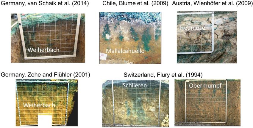
1832                                                               B. Berkowitz and E. Zehe: Surface water and groundwater

tropy is maximized and Gibbs free energy is minimized, be-           lated patterns. The emergence and persistence of preferential
cause all gradients have been dissipated by irreversible pro-        pathways even in homogeneous sand packs (e.g. Hoffman et
cesses. Hydrological systems are, however, open systems, as          al., 1996; Oswald et al., 1997; Levy and Berkowitz, 2003) is
they exchange mass (water, chemicals, sediments, colloids),          a striking example of formation of a self-organized pattern of
energy, and entropy across their system boundaries with their        “smooth fluid pressure gradients”.
environment. Hydrological systems may hence persist in a                Our general recognition is that hydrological systems ex-
state far from thermodynamic equilibrium. They may even              hibit – below and above ground – both (structural, hy-
evolve to states of a lower entropy, and thus stronger spa-          draulic, and chemical) heterogeneity and signatures of
tial organization, for instance through the steepening of gra-       (self-)organization. We propose that all kinds of preferen-
dients, in topography for example, or in the emergence of            tial flow paths and flow networks veining the land surface
structured variability of system characteristics or network-         and the subsurface are prime examples of spatial organiza-
like structures. Such a development is referred to as “self-         tion (Bejan et al., 2008; Rodriguez-Iturbe and Rinaldo, 2001)
organization” (Haken, 1983) because local-scale dissipative          because they exhibit, independently of their genesis, similar
interactions, which are irreversible and produce entropy, lead       topological characteristics. Our starting point to unify both
to ordered states or dynamic behaviour at the (macro-)scale          water worlds is the recognition that any form of preferen-
of the entire system. Self-organization requires free energy         tial flow is a manifestation of self-organization, because it
transfer into the system to perform the necessary physical           hinders perfect mixing within a system and implies a more
work, self-reinforcement through a positive feedback to as-          “energy-efficient” and hence faster throughput of water and
sure “growth” of the organized structure or patterns in space,       matter (Rodriguez-Iturbe et al., 1999; Zehe et al., 2010; Klei-
and the export of the entropy which is produced within the           don et al., 2013). This general notion can be elaborated fur-
local interactions to the environment (Kleidon, 2012).               ther by detailing the role of preferential flow for the trans-
   Manifestations of self-organization in catchment systems          port of mass and chemical species, and related fingerprints in
are manifold. The most obvious one is the persistence of             travel distances or travel times, as well as for energy conver-
smooth topographic gradients (Reinhardt and Ellis, 2015;             sion and energy dissipation associated with flows of water.
Kleidon et al., 2012), which reflect the interplay of tectonic          In terms of models, hydrological modelling (and hydro-
uplift and the amount of work water and biota have per-              logical theory) attempts to predict how processes described
formed to weather and erode solid materials, to form soils           by equations evolve in and interact with a structured hetero-
and create flow paths. Although these processes are dissi-           geneous domain (i.e. hydrological landscape). However, our
pative and produce entropy, they nevertheless leave signa-           key argument that both systems are subject to similar man-
tures of self-organization in catchment systems. These are           ifestations of self-organization does not imply proposed use
expressed, for instance, through the soil catena – a largely de-     of a single model. Rather, we argue that similar conceptual-
terministic arrangement of soil types along the topographic          izations and methods of quantification – whether related to
gradient of hillslopes (Milne, 1936; Zehe et al., 2014) –            preferential flow paths, dynamics and patterning of chemical
and even more strongly through the formation of rill and             transport and reactivity, or characterization in terms of en-
river networks (Fig. 1) at the hillslope and catchment scales        ergy dissipation and entropy production, for example – can
(Howard, 1990; Paik and Kumar, 2010; Kleidon et al., 2013).          and should be applied to both catchment and groundwater
These networks form because flow in rills is, in comparison          systems, to the benefit of both research communities. The
to sheet flow, associated with a larger hydraulic radius, which      main focus of this contribution is on the role of heterogene-
implies less frictional energy dissipation per unit volume of        ity and preferential flow and transport of water and chemical
flow. This causes higher flow rates, which in turn may erode         species. At a general level, we show that preferential flow
more sediment. As a result, these networks commonly in-              causes deviations from the maximum-entropy state, though
crease the efficiency in transporting water, chemicals, sedi-        these deviations have different manifestations depending on
ments and energy through hydrological systems, which also            whether we observe solute transport in space or in time.
results in increased kinetic energy transport through the net-       Based on this insight, we propose, essentially, that related
work and across system boundaries.                                   conceptualizations and quantitative characterizations can be
   In contrast, the term self-organization is rarely applied         unified in terms of a theory that is applicable in catchment
to groundwater systems, except in the context of positive            and groundwater systems and thus connects these two water
or negative feedbacks during processes of precipitation and          worlds.
dissolution (e.g. Worthington and Ford, 2009). We argue,                We first discuss key features of fluid flow and chemical
though, that the subsurface, too, displays some characteris-         transport dynamics in these two systems – catchments (in-
tics of (partial) self-organization. This is manifested, in par-     cluding surface water) and groundwater – using the (often
ticular, through ubiquitous, spatially correlated, anisotropic       distinct) terminology of each of these water world research
patterns of aquifer structural and hydraulic properties, par-        communities. We outline the particular questions, methods,
ticularly in non-Gaussian systems (Bardossy, 2006), as these         limitations, and uncertainties in each “world” (Sect. 2). We
have a much smaller entropy compared to spatially uncorre-           then focus on chemical transport, merging treatment of many

Hydrol. Earth Syst. Sci., 24, 1831–1858, 2020                                     www.hydrol-earth-syst-sci.net/24/1831/2020/
B. Berkowitz and E. Zehe: Surface water and groundwater 1833
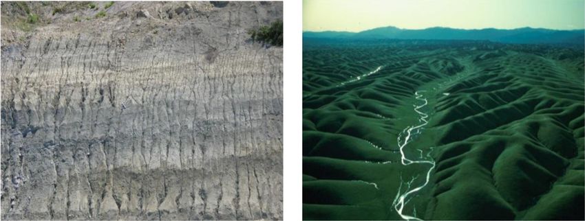
Figure 1. Hillslope-scale rill networks developed during an overland flow event at the Dornbirner Ach in Austria (left panel; we gratefully
acknowledge the copyright holder © Ulrike Scherer, KIT) and the South Fork of Walker Creek in California (right panel; we gratefully
acknowledge the copyright holder © James Kirchner, ETH Zürich).
of these dynamics in a proposed quantitative framework, pro- 2 Two water worlds – unique, different, and similar
viding specific examples (Sect. 3). More specifically, Sect. 3
first defines specific conceptual and quantitative tools and, 2.1 Governing laws of fluid flow, the momentum
within this context, introduces a continuous time random balance, and energy dissipation
walk (CTRW) modelling framework with a clear connec-
tion to microscale physics and to the well-known advection– In both water worlds, a major focus is on travel distances,
dispersion equation. Section 3 then offers new insights, in as well as travel times (residence times) of water, as they
terms of contrasting power law and inverse gamma distri- provide the main link between water quantity and quality
butions – used in the groundwater literature to describe dif- (Hrachowitz et al., 2016). Catchment hydrology also deals
ferent travel time distributions that control long tailing in with extremes, i.e. floods and droughts, as well as land
breakthrough curves – as well as gamma distributions used surface–atmosphere feedbacks, fluvial geomorphology, and
more often in the surface water (catchment system) litera- eco-hydrology.
ture. This analysis is a basis for suggesting how surface water From the outset, we recognize that predictions of water dy-
systems (catchment response to chemical transport) can be namics in catchment and aquifer systems require joint treat-
treated within the CTRW framework. Final conclusions and ment of their mass, momentum, and energy balances. Catch-
perspectives appear in Sect. 4. Throughout, we attempt to of- ment science and modelling has, traditionally, a strong focus
fer an innovative synthesis of concepts and methods from the on catchment mass and (in part) energy balances, as evapo-
generally disparate surface water (catchment hydrology) and ration and transpiration release energy in the form of latent
groundwater research communities. Each community has de- heat to the atmosphere. The momentum balance is treated in
veloped sophisticated modelling and measurement capabili- an implicit conceptualized manner, as detailed below. Predic-
ties – which have led to significant scientific advances over tions of fluid flow in groundwater systems rely on the joint
the last two decades – that could benefit the other community treatment of the mass and the stationary momentum balances
and help address outstanding, unsolved problems. using Darcy’s law, while the energy balance appears at first
Before proceeding, we emphasize that our use of the term sight to be of low importance.
“two water worlds” throughout this paper is intended to high- Chemical transport and travel times through hydrological
light the disparate catchment and groundwater communities, systems are, however, strongly related to both the momen-
and is not used in the specific context of mobile–immobile tum and the energy balances, because they jointly control the
water in the root zone (McDonnell, 2014), as discussed at spectrum of fluid velocities and the direction of streamlines.
the end of Sect. 3.1. The governing equations that characterize water flow veloc-
ities along the land surface and in groundwater systems are
simplifications of the Navier–Stokes equations (Eq. 1), which
describe the momentum balance of the fluid as an interplay
of driving forces and hindering frictional forces:
www.hydrol-earth-syst-sci.net/24/1831/2020/ Hydrol. Earth Syst. Sci., 24, 1831–1858, 2020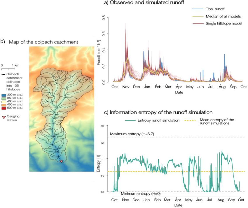
1834                                                                B. Berkowitz and E. Zehe: Surface water and groundwater

                                                                      of Darcy’s law (Eq. 3). The latter is also a steady-state, one-
                                                                      dimensional approximation of the Navier–Stokes equation
    ∂v
ρ      + (v · ∇) v = −∇p − ρg + η12 v,                       (1)      neglecting the inertial terms. However, in this case flow is
    ∂t                                                                essentially laminar and dissipative frictional losses in the
                                                                      porous medium are so much larger than in open surface flow
where v (m s−1 ) is the fluid velocity vector, g (m s−2 ) the
                                                                      that kinetic energy can be neglected. When solving Darcy’s
gravitation acceleration vector, ρ (kg m−3 ) the water density,
                                                                      law (Eq. 3, first line) for the interstitial travel velocities and
and η the dynamic viscosity (kg m−1 s−1 ) of the fluid.
                                                                      defining the flow resistance as inverse hydraulic conductivity,
2.1.1    Surface water flow and Manning’s law                         one obtains a form of Darcy’s law (Eq. 3, second line) which
                                                                      is similar to Manning’s law (Eq. 2). The main difference
Overland and channel flow are driven by surface topography,           arises from the different dependencies on the hydraulic head
or more precisely, by gravitational potential energy differ-          gradient, reflecting the turbulent and laminar flow regimes,
ences. But only minute amounts of these energy differences            respectively:
are converted into kinetic energy of the flow (Loritz et al.,         q vadose = −k (θ ) ∇ (ψ + z) , q gw = −ks ∇ (H + z) ,
2019), while the rest is dissipated. Surface water flow veloc-
ity is often characterized by Manning’s law (Eq. 2), a steady-                       1                            1
                                                                      v vadose = −         ∇8vadose , v gw = −        ∇8gw ,
state, one-dimensional approximation of the Navier–Stokes                         θ R (θ )                     θ s Rs
equation that neglects inertial acceleration for the case of          R (θ ) = 1/k(θ ), R = 1/ks ,
turbulent shear stress and thus turbulent energy dissipation.         8vadose = (ψ + z) , 8gw = (H + z) ,                           (3)
Fluid velocity grows proportionally to the square root of the
driving hydraulic head gradient; the latter corresponds to the        where q vadose and q gw (m s−1 ) are water flux vectors (filter
potential energy of a unit mass of water:                             velocities) in the partially saturated and saturated zones, re-
                                                                      spectively, v vadose and v gw (m s−1 ) are the respective inter-
                 2                         2
                R3 p                    R3 p                          stitial travel velocities, θ and θs are the soil water content
v surface = −        2g∇x,y (h + z) = −      2g∇x,y 8H , (2)          (–) and the porosity (–), k(θ ) and ks (m s−1 ) are the partially
                n                       n
                                                                      saturated and saturated hydraulic conductivity, ψ (m) and H
where v surface (m s−1 ) is the overland flow velocity vector,        (m) denote the capillary pressure and pressure potentials, and
R (m) the hydraulic radius defined as the ratio of the wetted         8vadose and 8gw are total hydraulic heads in the partially sat-
cross section Awet (m2 ) to the wetted perimeter Uwet (m),            urated and saturated zones.
n is Manning’s roughness (m−1/3 ), z (m) is topographical                The strikingly high dissipative nature of porous media flow
elevation, h (m) is depth of the flow, and 8 (m) is the total         becomes obvious when recalling that the driving matric po-
hydraulic head.                                                       tential gradients in the vadose zone are often orders of mag-
   Moreover, as friction occurs mainly at the contact line be-        nitude larger than 1 m m−1 . This implies a capillary accelera-
tween the fluid and the solid, the hydraulic radius R (m)             tion term much larger than Earth’s gravitational acceleration
can be used to scale the ratio between driving gravity force          g (m s−2 ), yet fluid velocities in the porous matrix are sev-
and the hindering frictional dissipative force. Kleidon et            eral orders of magnitude smaller than in surface water sys-
al. (2013) classified this as a “weak form” of dissipative inter-     tems. However, the generally much slower fluid velocity in
action between fluid and solid. In this context, they showed          groundwater systems does not impose a slow hydraulic re-
that overland flow in rills implies, due to the larger hydraulic      sponse time during rainstorms; on the contrary, aquifers may
radius, a smaller dissipative loss per unit volume and thus           release – almost instantaneously – “older”, pre-event water
a higher energy efficiency compared to sheet flow. Along              into a catchment outlet stream. This apparent paradox – often
the same line, they showed that flow in a smaller number              referred to as the “old–new water paradox” (Kirchner, 2003)
of wider channels is more efficient than flow in a higher             – is explained by propagation of pressure waves. Shear or
number of narrower channels. Both effects, flow in rills and          compression waves (or waves in general) transport momen-
channelling, lead to a higher fluid velocity, and thus a higher       tum and energy through continua without an associated trans-
power (kinetic energy flux) through the network. Note that            port of mass or particles (Everett, 2013; Goldstein, 2013),
a 10 % faster fluid velocity implies 30 % more power as the           and group velocity (or “celerity”) is many orders of magni-
latter grows with the cube of the fluid velocity.                     tude larger than the fluid velocity in aquifer systems (Mc-
                                                                      Donnell and Beven, 2014). Today, it is known that depend-
2.1.2    Subsurface flow and Darcy’s law                              ing on landscape setting, antecedent wetness conditions, and
                                                                      the dominant runoff mechanisms, pre-event water fractions
Flow through subsurface porous media, on the other hand, is           in storm runoff can vary from near zero to more than 60 % of
driven by the gradient in total hydraulic head, reflecting dif-       storm water, having an isotopic signature different from that
ferences in gravitational potential, matric potential, and pres-      of rainfall (Sklash and Farvolden, 1979; Sklash et al., 1996;
sure potential energies as described in the respective forms          Blume et al., 2008).

Hydrol. Earth Syst. Sci., 24, 1831–1858, 2020                                        www.hydrol-earth-syst-sci.net/24/1831/2020/
B. Berkowitz and E. Zehe: Surface water and groundwater                                                                       1835

2.1.3   Preferred flow paths as maximum power                       2.2     Catchment hydrology from the water balance to
        structures and non-Fickian transport                                solute transport

Flow velocity within subsurface preferential pathways               2.2.1    The catchment concept and the duality in water
(macropores, pipes, fractures) is known to be much faster                    balance modelling
than matrix flow (Beven and Germann, 1982, 2013). This is
caused not only by the vanishing capillary forces, but also,        Catchment hydrology developed largely as an engineering
largely, by the strong reduction in frictional dissipation in       discipline around traditional tasks of designing and operating
macropores compared to flow in the porous matrix. Viscous           reservoirs, flood risk assessment, and water resources man-
dissipation in preferential pathways occurs, similar to open        agement (Sivapalan, 2018). Although the catchment concept
channel flow, mainly at the contact line between fluid and          is elementary to these tasks, we think it worthwhile to reflect
solid, i.e. the wetted perimeter of the macropore, which im-        briefly on it here. The watershed boundary delimits a con-
plies – similar to the case of rill and river networks – a          trol volume where the streamlines are expected to converge
larger hydraulic radius and thus a much more energy-efficient       into the river network, and hence ideally the entire set of sur-
flow (Zehe et al., 2010). Darcy’s law is hence inappropriate        face and subsurface runoff components feeds the stream. We
to characterize preferential flow (Germann, 2018). Clearly,         can thus characterize the water balance of an ideally closed
rapid localized flow and transport in preferential pathways         catchment control volume based on observations of rainfall
hinders the transition from imperfectly mixed stochastic ad-        input and streamflow response (with uncertainty). Even more
vective transport in the near field to well-mixed advective–        importantly, the catchment water balance can be solved with-
dispersive transport in the far field. Predictions of solute        out an explicit treatment of the momentum balance, because
plumes and travel times in the near field are thus challeng-        flow lines end up in the stream.
ing as this requires detailed knowledge of the velocity field,         This is a twofold blessing. First, hydrological models can
while transport at the well-mixed Fickian limit depends on          be benchmarked against integral water balance observations.
the average fluid velocity and the dispersion coefficient (Sim-     We posit that this unique property of catchments is the reason
mons, 1982; Sposito et al., 1986; Bodin, 2015).                     why integral conceptual hydrological models, which largely
   Although the revisited laws, interactions, and phenomena         ignore the momentum balance, allow successful predictions
are well known, we suggest that an energy-centred point of          of streamflow to the catchment outlet (Sivapalan, 2018). As
view yields a unifying perspective to explain why macropore,        conceptual models directly address processes at the system
rill, and river networks are the preferred (preferential) path-     level without accounting for sub-scale mechanistic reasons,
ways for water flow on land and below. One might hence              their application is often referred to as “top-down” mod-
expect that water flows along the path of maximum power             elling. The other end of the model spectrum consists of
(Howard, 1990; Kleidon et al., 2013), which is the product          physics-based, spatially distributed models, originally pro-
of the flow velocity times the driving potential difference.        posed by the blueprint of Freeze and Harlan (1969), which
The paths of maximum power correspond in the case of con-           follow a “bottom-up” mechanistic paradigm. These models
stant friction to the path of steepest descent in hydraulic head,   are thus also referred to as reductionist models. While the
while in the case of a constant gradient, it corresponds to the     pros and cons of top-down conceptual models and bottom-
path of minimum flow resistance (Zehe et al., 2010). From           up physics-based models have been discussed extensively,
the discussion above, we further conclude that catchment hy-        we agree with Hrachowitz and Clark (2017) that they offer
drology and groundwater hydrology are inseparable. We can           complementary merits, as detailed below. As an aside, it is
separate neither a river from its catchment and its subsurface      interesting to reflect why conceptual models due not exist in
nor an aquifer from the land surface and the catchment. Both        the field of, for example, meteorology. We suggest that this
streamflow response to rainfall and groundwater are com-            is because atmospheric flows are not governed by organized
posed of “waters of different ages”, reflecting the ranges of       structures acting similarly to catchments, which implies that
overland flow, subsurface storm flow, and base-flow contribu-       the amount of air mass flowing from one location to another
tions with their specific velocities, usually non-Fickian travel    cannot be predicted without knowing the flow lines.
time distributions, and chemical signatures.
   In the following, we elaborate briefly on the specific model     2.2.2    Top-down modelling of the catchment water
paradigms in catchment and groundwater hydrology with an                     balance
emphasis on preferential pathways for fluid flow and chem-
ical transport, and on the resulting ubiquitous, anomalous          Top-down conceptual hydrological models simulate water
early and late arrivals of chemicals to measurement outlets.        storage, redistribution, and release within the catchment sys-
                                                                    tem through a combination of non-linear and linear reser-
                                                                    voirs, characterized by effective state variables and effec-
                                                                    tive parameters and effective fluxes (Savenije and Hra-
                                                                    chowitz, 2017). Due to their mathematical simplicity, con-

www.hydrol-earth-syst-sci.net/24/1831/2020/                                       Hydrol. Earth Syst. Sci., 24, 1831–1858, 2020
1836                                                              B. Berkowitz and E. Zehe: Surface water and groundwater

ceptual models are straightforward to code. With the advent         anisms are represented through an appropriate combination
of combinatorial optimization methods for automated param-          of these conceptual “building blocks” (Fenicia et al., 2014;
eter search, and fast computers (Duan et al., 1992; Bárdossy        Gao et al., 2014; Wrede et al., 2015) using suitable topo-
and Singh, 2008; Vrugt and Ter Braak, 2011), these models           graphical signatures such as “height above next drainage”
also became, at first sight, straightforward to apply. Auto-        (Gharari et al., 2011) to estimate their areal share. This is a
mated, random parameter search led, however, to the discov-         clear advantage that facilitates model calibration and reduc-
ery of the well-known equifinality problem – namely, that           tion of predictive uncertainty.
several model structures or parameter sets may reproduce               The strength of integral conceptual models is their ability
the target data in an acceptable manner (Beven and Binley,          to provide parsimonious and reliable predictions of stream-
1992), within the calibration and validation period, but these      flow Q (m3 s−1 ) directly at the catchment outlet. However, it
models and parameter sets yield uncertain future predictions        is nevertheless not straightforward to apply these models for
(e.g. Wagener and Wheater, 2006). Equifinality and related          predictions of transport of tracers, and more generally chemi-
parameter uncertainty arises from the ill-posed nature of in-       cal species through the catchment into a stream, as elaborated
verse parameter estimation and from parameter interactions          in the following.
in the equations. While the first problem can be tackled using
multi-objective and multi-response calibration (e.g. Mertens        2.2.3   Integral approaches to solute transport modelling
et al., 2004; Ebel and Loague, 2006; Fenicia et al., 2007), the             in catchment hydrology
latter is inherent to the model equations regardless of whether
they are conceptual (as shown by Bárdossy, 2007, for the            Predictions of solute transport require information about the
Nash cascade) or physically based (as shown by Klaus and            spectrum of fluid velocities and travel distances across the
Zehe, 2010, and Zehe et al., 2014, for example).                    various flow paths into the stream (we can usually neglect
   A well-known shortcoming of conceptual models is that            the travel time within the river network due to the much
their key parameters cannot be measured directly. This mo-          higher fluid velocities, as argued in Sect. 3.1). Such informa-
tivated numerous parameter regionalization efforts (He et           tion can generally be inferred from breakthrough curves of
al., 2011a) to relate conceptual parameters to measurable           tracers that enter and leave the system through well-defined
catchment characteristics, typically broadly available data         boundaries, as shown for instance by the early work of Sim-
on soils (including texture), land use, and topography. As          mons (1982) and Jury and Sposito (1986), using transfer
a consequence, such functions have been derived success-            functions to model solute transport through soil columns.
fully, for example, to relate parameters of the soil moisture       The transfer function approach is based on the theory of lin-
accounting scheme to soil type and land use (as shown by,           ear systems. This implies that the outflow concentration (vol-
for example, Hundecha and Bardossy, 2004; Samaniego and             umetric flux-averaged concentration) Cout (kg m−3 ) at time t
Bardossy, 2006; He et al., 2011b; and Singh et al., 2016)           is, in the case of steady-state water flow, the convolution of
or parameters of the soil moisture accounting of the mHm            the solute input time series Cin with the system function G
(Samaniego et al., 2010) to soil textural data. As these re-        (Green’s function):
lations are landscape-specific, they require a new calibration                Z∞
when moving to new target areas. This is of course possible if
                                                                    Cout (t) = G (t − τ ) Cout (τ ) dτ.                        (4)
high quality discharge data are available. Yet, due to the in-
compatibility between the corresponding measurement and                        0

observations scales, these regionalization functions are not           The transfer function is the system response to a delta
straightforwardly explained using physical reasoning. This          function input. Note that Eq. (4) should in general be formu-
is true even if soil moisture accounting from soil physics is       lated for the input and output mass flows, which correspond
used, e.g. the Brooks and Corey (1964) soil water retention         to the input–output concentration multiplied by the input–
curve, as in the case of the mHm model.                             output volumetric water flows. It is important to note in this
   A number of early efforts to meaningfully define                 context that the average travel time through the system can be
hydrological response units for regional modelling of               calculated from the water flow and length of flow path, as the
hydrological landscapes were reported by Knudsen et                 average travel velocity corresponds to the flow divided by the
al. (1986), Flügel (1995), and Winter (2001), for example.          wetted cross section of the soil column (see Eq. 3). The latter
Savenije (2010) and Fencia et al. (2011) significantly im-          implies that travel time distributions through partially satu-
proved the link between conceptual models and landscape             rated soils are transient and hence constrained by the input
structure in their flexible model framework. The key idea           time (Jury and Sposito, 1986; Sposito et al., 1986). The well-
is to subdivide the landscape into different functional units       known fact that the flow velocity field changes continuously
(plateaus, hillslopes, wetlands, rivers), and to represent each     with changing soil water content explains why transfer func-
of them by a specific combination of conceptual model com-          tion approaches have been largely put aside in soil physics
ponents to mimic their dominant runoff generation processes.        and solute transport modelling in the partially saturated zone.
Landscapes with different dominant runoff generation mech-

Hydrol. Earth Syst. Sci., 24, 1831–1858, 2020                                      www.hydrol-earth-syst-sci.net/24/1831/2020/
B. Berkowitz and E. Zehe: Surface water and groundwater                                                                        1837

   In the case of catchments, simulated runoff from concep-         Klaus, 2019); others used the beta distribution (van der Velde
tual hydrological models cannot, unfortunately, be used to          et al., 2012) or piece-wise linear distributions (Hrachowitz et
constrain the average transport velocity. This is simply be-        al., 2013, 2015).
cause conceptual models provide, by definition, no infor-              Here we propose that the CTRW framework from the
mation about the wetted cross of the flow path through the          groundwater “world” has much to offer to catchment travel
catchment, and the latter determines essentially the average        time modelling (as detailed in Sect. 3). We show that, in par-
fluid velocity v from simulated total runoff Q. The fact that       ticular, the inverse gamma distribution may offer a useful
the simple equation Q = vtransport Awet has an infinite solu-       alternative that offers the asset of a clear connection to mi-
tion space, if Awet is unknown, is also a major source of           croscale physics and the well-known advection–dispersion
equifinality. This was shown by Klaus and Zehe (2010) and           equation, which is used in bottom-up modelling (Sect. 2.2.4).
Wienhöfer and Zehe (2014), using a physically based hydro-          In this context, it is interesting to recall that catchments were
logical model to investigate the role of vertical lateral prefer-   modelled as time-invariant linear systems for a considerable
ential flow paths of hillslope rainfall–runoff response. These      time, since the unit hydrograph was introduced by Sher-
authors found that several network configurations matched           man (1932). While the effect of precipitation was calculated
the observed flow response equally well: some configura-            using runoff coefficients, the streamflow response was sim-
tions consisted of a small number of larger macropores of           ulated by convoluting effective precipitation with the system
higher conductance, while others consisted of a higher num-         function, i.e. the unit hydrograph. The “Nash” cascade of lin-
ber of less conductive macropores. Overall, these configura-        ear reservoirs was a popular means to describe the unit hy-
tions yielded the same volumetric water flow, but they per-         drograph in a parametric form, and it is well known that the
formed rather differently with respect to the simulation of         latter is mathematically equivalent to a gamma distribution
solute transport. An even larger challenge for transport mod-       (Nash, 1957). As streamflow response of the catchment is
elling through catchments arises from the fact that the distri-     affected largely by surface and subsurface preferential path-
bution of flow path lengths is even more difficult to constrain,    ways, which cause non-Fickian transport, one might hence
compared to a soil column.                                          wonder whether a gamma distribution function is an ideal
   Despite these challenges, the tracer hydrology commu-            choice to represent the fingerprint of preferential flow.
nity made considerable progress in understanding catchment
transit time distributions and predicting isotope or tracer con-    2.2.4   Bottom-up modelling of the catchment water
centrations in streamflow (Harman, 2015). Initially, stable                 balance
isotopologues of the water molecule and other tracers gained
attention as they allow a separation of the storm hydrograph        The blueprint of a physically based hydrology, introduced by
into pre-event and event water fractions using stable end           Freeze and Harlan (1969), has found manifold implementa-
member mixing (Bonell et al., 1990; Sklash et al., 1996).           tions. Physically based models like MikeShe (Refsgaard and
Today isotopes of the water molecules and water chemistry           Storm, 1995) or CATHY (Camporese et al., 2010) typically
data are used as a continuous source of information to infer        rely on the Darcy–Richards equation for soil water dynamics
travel time distributions of water through catchments (McG-         (Eq. 3), the Penman–Monteith equation for soil–vegetation–
lynn et al., 2002; McGlynn and Seibert, 2003; Weiler et al.,        atmosphere exchange processes, and the Manning’s equation
2003; Klaus et al., 2013). Early attempts to predict tracer         for estimating overland and streamflow velocities (Eq. 2).
concentrations in the stream relied on the same kind of trans-         Each of these approaches is naturally subject to limita-
fer functions as outlined in Eq. (4) for soil columns. Hence,       tions, reflecting our yet imperfect understanding, and suffers
they naturally faced the same problems of state and thus            from the limited transferability of their related parameters
time-dependent travel time distributions (Hrachowitz et al.,        from idealized, homogeneous laboratory conditions to het-
2013; Klaus et al., 2015; Rodriguez et al., 2018). More re-         erogeneous and spatially organized natural systems (Grayson
cent approaches rely on age-ranked storage as a “state” vari-       et al., 1992; Gupta et al., 2012). In this context, the Darcy–
able in combination with storage selection (SAS) functions          Richards model has received by far the strongest criticism
for streamflow and evapotranspiration to infer their respec-        (Beven and Germann, 2013), simply because the under-
tive travel time distributions (Harmann, 2015; Rinaldo et al.,      lying assumption regarding the dominance of capillarity-
2015). Aged ranked storage needs to be inferred from solving        controlled diffusive flow, under local equilibrium conditions,
the master equation, i.e. the catchment water balance for each      is largely inappropriate when accounting for preferential
time and each age. This can be done by using either concep-         flow. The Darcy model is hence incomplete when account-
tually modelled or observed discharge and evapotranspira-           ing for infiltration (Germann, 2018) and preferential flow,
tion, and it requires a proper selection of the functional form     and several approaches have been proposed to close this gap.
of the SAS functions and optionally their time-dependent            These range from (a) the early idea of stochastic convec-
weights (Rodriguez and Klaus, 2019). Related studies rely on        tion assuming no mixing at all (Simmons, 1982), to (b) dual-
a single gamma distribution or several gamma distributions          permeability conceptualizations relying on overlapping, ex-
(Hrachowitz et al., 2010; Klaus et al., 2015; Rodriguez and         changing continua (Šimunek et al., 2003), to (c) spatially ex-

www.hydrol-earth-syst-sci.net/24/1831/2020/                                      Hydrol. Earth Syst. Sci., 24, 1831–1858, 2020
1838                                                                B. Berkowitz and E. Zehe: Surface water and groundwater

plicit representations of macropores as connected flow paths          catchment using 105 different hillslopes yielded strongly re-
(Vogel et al., 2006; Sander and Gerke, 2009; Zehe et al.,             dundant contributions of streamflow (Fig. 2). The Shannon
2010; Wienhöfer and Zehe, 2014; Loritz et al., 2017), and             entropy (Shannon, 1948, defined in Eq. 6 in Sect. 2.4) was
to (d) pore-network models based on mathematical morphol-             used to quantify the diversity in simulated runoff of the hills-
ogy (Vogel and Roth, 2001). An alternative approach to deal-          lope ensemble at each time step. They found that although
ing with preferential flow and transport employs Lagrangian           the entropy of the ensemble was rather dynamic in time,
models such as SAMP (Ewen, 1996a, b), MIPs (Davies and                it never reached the maximum value. Note that an entropy
Beven, 2012; Davies et al., 2013), and LAST (Zehe and Jack-           maximum implies that hillslopes contribute in a unique fash-
isch, 2016; Jackisch and Zehe, 2018; Sternagel et al., 2019).         ion, while a value of zero implies that all hillslopes yield a
    Reductionist models are, despite the challenge to represent       similar runoff response. They further showed that the fully
preferential flow and transport, indispensable tools for scien-       distributed model, consisting of 105 hillslopes, can be com-
tific learning. They particularly allow the exploration of how        pressed to a model using 6 hillslopes with distinctly different
distributed patterns and their spatial organization jointly con-      runoff responses, without a loss in simulation performance.
trol distributed state dynamics and integral behaviour of hy-         Based on these findings, they concluded that spatial organi-
drological systems (Zehe and Blöschl, 2004). Related stud-            zation leads to the emergence of functional similarity at the
ies include the investigation of (a) how changes in agricul-          hillslope scale, as proposed by Zehe et al. (2014). This in
tural practices affect the streamflow generation in a catch-          turn explains why conceptual models can be reasonably ap-
ment (Pérez et al., 2011), (b) the role of bedrock topogra-           plied, as most of the spatial heterogeneity in the catchment
phy for runoff generation (Hopp and McDonnell, 2009) at               seems to be irrelevant for runoff production. However, this is
the Panola hillslope and the Colpach catchment (Loritz et al.,        not the case when it comes to the transport of chemicals, as
2017), and (c) the role of vertical and lateral preferential flow     elaborated in the next section.
networks on subsurface water flow and solute transport at                In accord with Hrachowitz and Clark (2017), we conclude
the hillslope scale (Bishop et al., 2015; Wienhöfer and Zehe;         that top-down and bottom-up models indeed have comple-
2014; Klaus and Zehe, 2011, 2010), including the issue of             mentary merits. Moreover, we propose that the applicability
equifinality. Setting up a physically based model, however,           of conceptual models at larger scales arises from the fact that
requires an enormous amount of highly resolved spatial data,          spatial organization leads in conjunction with the strongly
particularly on subsurface characteristics. Such data sets are        dissipative nature of hydrological process to the emergence
rare, and the “hunger” for data in such models risks a much           of simplicity at larger scales (Savenije and Hrachowitz, 2017;
higher structural model uncertainty. On the other hand, these         Loritz et al., 2018).
models also offer greater opportunities for constraining their
structure using multiple data orthogonal to discharge (Ebel           2.3   Distributed solute transport modelling – the key
and Loague, 2006; Wienhöfer and Zehe, 2014).                                role of the critical zone
    Another asset of reductionist models is their thermody-
namic consistency, which implies that energy conversions re-          Reductionist physically based models are straightforward
lated to flow and storage dynamics of water in the catchment          to couple with the advection–dispersion equation (compare
systems are straightforward to calculate (Zehe et al., 2014).         Eq. 11 in Sect. 3) or particle-tracking schemes to simulate
This offers the opportunity to test the feasibility of thermody-      transport of tracers and reactive compounds through the crit-
namic optimality as constraint for parameter inference (Zehe          ical zone into groundwater or along the surface and through
et al., 2013); the latter is rather challenging when using con-       the subsurface into the stream.
ceptual models (Westhoff and Zehe, 2013; Westhoff et al.,                The soil–vegetation–atmosphere–transfer system (SVAT
2016). More recent applications demonstrated, in line with            system), or in more recent terms, the “critical” zone, is the
this asset, new ways to simplify distributed models without           mediator between the atmosphere and the two water worlds.
lumping, which allowed the successful simulation of the wa-           This tiny compartment controls the splitting of rainfall into
ter balance of a 19 km2 large catchment using a single ef-            overland flow and infiltration, and the interplay among soil
fective hillslope model (Loritz et al., 2017). The key to this        water storage, root water uptake, and groundwater recharge.
was to respect energy conservation during the aggregation             Soil water and soil air contents control CO2 emissions of for-
procedure, specifically through derivation of an effective to-        est soils, denitrification, and related trace gas emissions into
pography that conserved the average distribution of potential         the atmosphere (Koehler et al., 2010, 2012), as well as bio-
energy along the average flow path length to the stream, and          geochemical transformations of chemical species.
through a macro-scale effective soil water retention curve               Partly saturated soils may, depending on their initial state
that conserved the relation between the average soil water            and structure, respond with preferential flow and transport
content and matric potential energy using a set point-scale           of contaminants and nutrients through the most biologi-
retention experiments (Jackisch, 2015; Zehe et al., 2019).            cally active topsoil buffer (Flury et al., 1994, 1995; Flury,
    Along similar lines, Loritz et al. (2018) showed that sim-        1996; McGrath et al., 2008, 2010; Klaus et al., 2014). Rapid
ulations using a fully distributed set-up of the same Colpach         transport operates within strongly localized preferential path-

Hydrol. Earth Syst. Sci., 24, 1831–1858, 2020                                       www.hydrol-earth-syst-sci.net/24/1831/2020/
B. Berkowitz and E. Zehe: Surface water and groundwater 1839 Figure 2. (a) Observed and simulated runoff of the Colpach catchment. The red lines correspond to individual hillslope models and the yellow line to the area-weighted median of all hillslopes. (b) Map of the Colpach catchment and the 105 different hillslopes. (c) Shannon entropy in turquoise for the runoff simulations as well as the corresponding mean. © Ralf Loritz, KIT; from Loritz et al. (2018). ways such as root channels, cracks, and worm burrows or fingers and/or long-term concentration tails in tracer profiles. within connected inter-aggregate pore networks which “by- Frequently, the partially saturated region of the subsurface is pass” the soil matrix continuum (e.g. Beven and Germann, simply too thin to allow perfectly mixed Gaussian travel dis- 1982, 2013; Blume et al., 2009; Wienhöfer et al., 2009). The tances to be established; hence non-Fickian transport in the well-known fingerprint of preferential flow is a “fingered” critical zone is today regarded as being the rule rather than flow pattern, which is often visualized through dye stain- the exception. ing or two-dimensional concentration patterns in vertical soil Because preferential transport leads to strongly localized profiles (Fig. 3). These reveal imperfectly mixed conditions accumulation of water and chemical species, preferential in the near field, which implies that the spatial concentra- pathways are potential biogeochemical hotspots. This is par- tion pattern deviates from the well-mixed Fickian limit over ticularly the case for biopores such as worm burrows and root a relatively long time. The latter corresponds in the case of a channels. Worm burrows provide a high amount of organic delta input to a Gaussian distribution of travel distances at a carbon and worms “catalyse” microbiological activity due fixed time, where the centre of mass travels with the average to their enzymatic activity (Bundt et al., 2001; Binet et al., transport velocity while the spreading of the concentration 2006; Bolduan and Zehe, 2006; van Schaik et al., 2014). Sim- grows linearly with time proportionally to the macrodisper- ilarly, plant roots provide litter and exude carbon substrates sion coefficient (Simmons, 1982; Bodin, 2015). Note that ac- to facilitate nutrient uptake. Intense runoff and preferential cording to Trefry et al. (2003) this Gaussian travel distance flow events optionally connect these isolated “hot spots” to corresponds to a state of maximum entropy. Preferential flow lateral subsurface flow paths such as a tile drain network or a hence implies a deviation from this well-mixed maximum- pipe network along the bedrock interface and thereby estab- entropy state, which cannot be predicted with the advection– lish “hydrological connectivity” (Tromp-van Meerveld and dispersion equation (e.g. Roth and Hammel, 1996). A re- McDonnell, 2006; Lehmann et al., 2007; Faulkner, 2008). cent study (Sternagel et al., 2019) revealed that even double- The onset of hydrological connectivity comprises again a domain models such as Hydrus 1D may fail to match the flow “hot moment” as upslope areas and, potentially, the entire www.hydrol-earth-syst-sci.net/24/1831/2020/ Hydrol. Earth Syst. Sci., 24, 1831–1858, 2020
1840 B. Berkowitz and E. Zehe: Surface water and groundwater
Figure 3. Finger flow pattern revealed from standardized dye staining experiments for a transport time of 1 d; images were generously
provided by Flury et al. (1994, 1995; © American Geophysical Union 1994, 1995) for Switzerland, Blume et al. (2009, © Theresa Blume)
for Chile, Wienhöfer et al. (2009, © Jan Wienhöfer, KIT) for Austria, and Zehe and Flühler (2001, © Erwin Zehe, KIT) and van Schaik et
al. (2014, © John Wiley & Sons, Ltd. 2013) for the German Weiherbach.
catchment start “feeding” the stream with water, nutrients, water at each scale – separating these pockets at the pore,
and contaminants (Wilcke et al., 2001; Goller et al., 2006). the column, the metre, the 10 m, and the field and catchment
The critical zone, furthermore, crucially controls the scales – we instead suggest recognizing and delineating an
Bowen ratio (the partitioning of net radiation energy into sen- “overall effect” of separation between “old” (immobile) and
sible and latent heat), and soil water available to plants is a “new” (mobile) waters at a given “effective” scale of inter-
key controlling factor. The residual soil water content is not est, which integrates over all such old and new waters. As we
available for plants, as it is generally stored in fine pores sub- discuss in detail at the end of Sect. 3.1 and thereafter, we ar-
ject to very high capillary forces. Isotopic tracers have been gue that it is a more effective approach to consider chemical
fundamental to unravelling water flow paths in soils, using transport as following distributions of travel distances and
dual plots (Benettin et al., 2018; Sprenger et al., 2018), and residence times, which can then be characterized by various
to distinguishing soil water that is recycled to the atmosphere (often power law) probability density functions (PDFs).
and released as streamflow (Brooks et al., 2010; McDonnell,
2014). 2.4 Groundwater systems
Further to the above points, it is noted that labora-
tory and numerical studies of multiple cycles of infiltra- As noted in Sect. 1, analysis of groundwater systems has de-
tion and drainage of water and chemicals into a porous veloped largely independently of the investigation of catch-
medium demonstrate clearly the establishment of stable ment systems, although it, too, developed originally as a
“old” water clusters or pockets, and even a “memory ef- large deterministic engineering discipline around the tradi-
fect” (Kapetas et al., 2014), which remain even with mul- tional task of water supply for domestic and agricultural use.
tiple cycles of “new” water infiltration (Gouet-Kaplan and It was only in the 1980s that “stochastic” (probabilistic and
Berkowitz, 2011). These pore-scale studies are in qualitative statistical) techniques began to be implemented extensively,
(and semi-quantitative) agreement with studies at the field to account for the many uncertainties associated with aquifer
scale, which show similar retention behaviour of bromide structure and hydraulic properties that control the flow of
(introduced during the first infiltration cycle) after multiple groundwater. In parallel, significant interest in (and con-
infiltration–drainage cycles (Turton et al., 1995; Collins et cern with) water quality and environmental contamination in
al., 2000). As a consequence, when each cycle of infiltra- groundwater systems only entered the research community’s
tion contains water with a different chemical signature, sta- consciousness in the 1980s, although some pioneering lab-
ble pockets of water can be established with highly vary- oratory experiments and field measurements were initiated
ing chemical composition. We hence emphasize that mobile from the late 1950s.
and immobile waters sustaining evaporation and streamflow It is worth noting, too, that the methods and models ap-
– and the chemical species they contain – exist at a contin- plied in groundwater research developed independently and
uum of scales from the pore to the field level. Thus, rather separately from research on catchment systems (Sect. 1). The
than attempting to delineate pockets of less and more mobile only partial connection or “integrator” has traditionally been
with aquifer connections to the vadose zone (or critical zone,
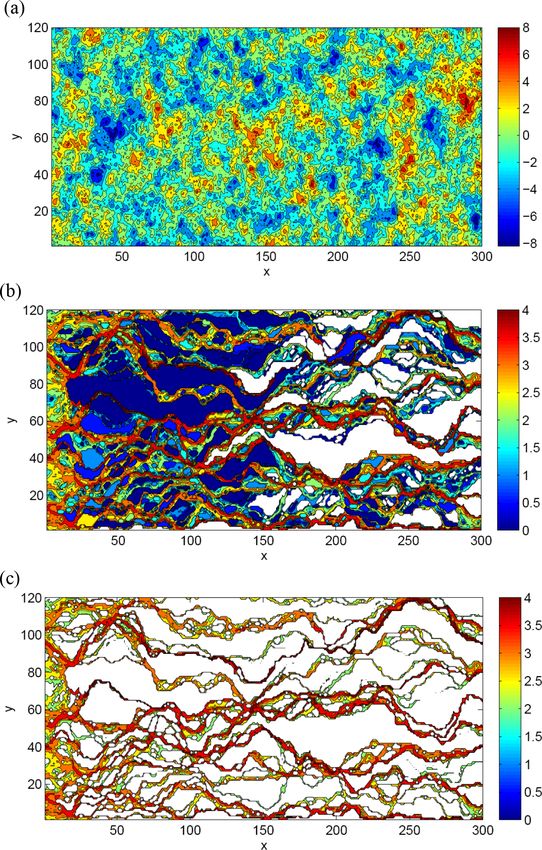
Hydrol. Earth Syst. Sci., 24, 1831–1858, 2020 www.hydrol-earth-syst-sci.net/24/1831/2020/B. Berkowitz and E. Zehe: Surface water and groundwater 1841 discussed in Sect. 2.3). Another connection between surface reaction (sorption, complexation, transformation) – so that water and groundwater systems, though not generally rec- chemical migration through an aquifer is influenced strongly ognized as such, has been analysis of water flow, and to by aquifer heterogeneities and initial or boundary conditions. a lesser extent chemical species transport, in the hyporheic Extensive analysis of high-resolution experimental measure- zone. The hyporheic zone can be defined as the region of sed- ments and numerical simulations of transport demonstrate iment and subsurface porous domain below and adjacent to that small-scale heterogeneities can significantly affect large- a streambed, which enables mixing of shallow groundwater scale behaviour, and that small-scale fluctuations in chem- and surface water (e.g. Haggerty et al., 2002). ical concentrations do not simply average out and become To quantify chemical transport, landmark laboratory ex- insignificant at large scales. periments (e.g. Aronofsky and Heller, 1957; Scheidegger, As discussed in the preceding sections, preferential path- 1959) measured the breakthrough of conservative (non- ways are ubiquitous and affect both water and chemical reactive) chemical tracers through columns of sand. These species, resulting from system heterogeneity. To be more measurements underpinned theoretical developments, also specific, (local) hydraulic conductivities vary in space over based on concepts of Fickian diffusion, which led to con- orders of magnitudes, even within distances of centimetres sideration of the classical advection–dispersion equation. to metres, and these variations ultimately control patterns Since that time, the advection–dispersion equation – and of fluid and chemical movement. The resulting patterns of variants of it – have been used extensively to quantify movement in these systems involve highly ramified prefer- chemical transport in porous media. However, as thor- ential pathways for water movement and chemical migration. oughly discussed in Berkowitz et al. (2006), solutions of To illustrate these points, consider the hydraulic conductiv- the advection–dispersion equation have repeatedly demon- ity (K) and preferential pathway maps shown in Fig. 4a; see strated an inability to properly match the results of exten- Edery et al. (2014) for full details. sive series of laboratory experiments, field measurements, Figure 4a shows a numerically generated, two- and numerical simulations. These findings naturally lead to dimensional domain measuring 300 × 120 discretized the conclusion that the conceptual picture underlying the grid cells of uniform size (0.2 units). The K field shown advection–dispersion equation framework is insufficient; as here was generated as a random realization of a statisti- detailed in Sect. 2.2, the soil physics community arrived at cally homogeneous, isotropic, Gaussian ln(K) field, with a similar conclusion. Stochastic variants of the advection– ln(K) variance of σ 2 = 5. Fluid flow through this domain dispersion equation and the implementation of multiple- was solved at the Darcy level by assuming constant head continua, advection–dispersion equation formulations (in- boundary conditions on the left and right boundaries, and cluding mobile–immobile models) have been used to provide no-flow horizontal boundaries; the hydraulic head values insights into factors that affect chemical transport – partic- determined throughout the domain were then converted to ularly given uncertain knowledge of detailed structural and local velocities, and thus streamlines. Conservative chemical hydraulic aquifer properties – but they have been largely un- transport was determined using a standard Lagrangian able to capture measured behaviour of chemical transport. particle-tracking method, with 105 particles representing This observation is largely in line with what we reported for the dissolved chemical species. Particles advanced by the critical zone. advection along the streamlines and molecular diffusion The first key is to recognize that heterogeneities are (enabling movement between streamlines), to generate present at all scales in groundwater systems, from sub- breakthrough curves (concentration vs. time) at various millimetre pore scales to the scale of an entire aquifer. In- distances throughout the domain. Figure 4b shows particle deed, use of the term “heterogeneities” refers to varying dis- pathways through the domain, wherein the number of tributions of structural properties (e.g. porosity, presence of particles visiting each cell is represented by colours. The fractures, and other lithological features), hydraulic proper- emergence of distinct, limited particle preferential pathways ties (e.g. hydraulic conductivity), and – in the case of chem- from inlet boundary to outlet boundary is striking. Notably, ical transport (a general term used here and throughout to too, there are significant regions that remain free of particles denote migration of chemical and/or microbial components) (the white regions in Fig. 4b), and preferential pathways are – variations in the biogeochemical properties of the porous confined and converge between low conductivity areas. Even domain medium. The second key is to recognize that these more striking is the set of even sparser preferential pathways variations in distributions, at all scales, deny the possibility shown in Fig. 4c: here, only cells which were visited by of obtaining complete knowledge of the aquifer domain in at least 0.1 % of all injected particles are shown. In other which fluids and chemical species are transported. A third words, 99.9 % of all chemical species migrating through the key, when considering chemical transport (and transport of domain shown in Fig. 4a advance through a limited number stable water molecule isotopes), is to recognize that chem- and spatial extent of preferential pathways. It is significant, ical species are subject to several critical transport mech- too, that the preferential pathways comprise a combination anisms and controls, in addition to advection, that do not of higher conductivity cells in the paths, but also some low affect flow of water – molecular diffusion, dispersion, and www.hydrol-earth-syst-sci.net/24/1831/2020/ Hydrol. Earth Syst. Sci., 24, 1831–1858, 2020
You can also read