Airborne measurements of oxygen concentration from the surface to the lower stratosphere and pole to pole - Recent
←
→
Page content transcription
If your browser does not render page correctly, please read the page content below
Atmos. Meas. Tech., 14, 2543–2574, 2021
https://doi.org/10.5194/amt-14-2543-2021
© Author(s) 2021. This work is distributed under
the Creative Commons Attribution 4.0 License.

Airborne measurements of oxygen concentration from the surface to
the lower stratosphere and pole to pole
Britton B. Stephens1 , Eric J. Morgan2 , Jonathan D. Bent2,1,a , Ralph F. Keeling2 , Andrew S. Watt1 , Stephen R. Shertz1 ,
and Bruce C. Daube3
1 National Center for Atmospheric Research, Boulder, Colorado, USA
2 Geosciences  Research Division, Scripps Institution of Oceanography, La Jolla, California, USA
3 School of Engineering and Applied Sciences, Harvard University, Cambridge, Massachusetts, USA
a now at: Picarro, Inc., Santa Clara, California, USA

Correspondence: Britton B. Stephens (stephens@ucar.edu)

Received: 19 July 2020 – Discussion started: 28 August 2020
Revised: 3 January 2021 – Accepted: 14 January 2021 – Published: 1 April 2021

Abstract. We have developed in situ and flask sampling sys-        midity effects by comparison to the corrected flask values.
tems for airborne measurements of variations in the O2 /N2         A comparison of Ar/N2 -corrected Medusa flask δ(O2 /N2 )
ratio at the part per million level. We have deployed these        measurements to regional Scripps O2 Program station obser-
instruments on a series of aircraft campaigns to measure           vations shows no systematic biases over 10 recent campaigns
the distribution of atmospheric O2 from 0–14 km and 87◦ N          (+0.2 ± 8.2 per meg, mean and standard deviation, n = 86).
to 86◦ S throughout the seasonal cycle. The National Cen-          For AO2, after resolving sample drying and inlet fractiona-
ter for Atmospheric Research (NCAR) airborne oxygen in-            tion biases previously on the order of 10–100 per meg, in-
strument (AO2) uses a vacuum ultraviolet (VUV) absorp-             dependent AO2 δ(O2 /N2 ) measurements over six more re-
tion detector for O2 and also includes an infrared CO2 sen-        cent campaigns differ from coincident Medusa flask mea-
sor. The VUV detector has a precision in 5 s of ±1.25 per          surements by −0.3 ± 7.2 per meg (mean and standard devia-
meg (1σ ) δ(O2 /N2 ), but thermal fractionation and motion         tion, n = 1361) with campaign-specific means ranging from
effects increase this to ±2.5–4.0 per meg when sampling            −5 to +5 per meg.
ambient air in flight. The NCAR/Scripps airborne flask sam-
pler (Medusa) collects 32 cryogenically dried air samples per
flight under actively controlled flow and pressure conditions.
For in situ or flask O2 measurements, fractionation and sur-       1   Introduction
face effects can be important at the required high levels of
relative precision. We describe our sampling and measure-          Atmospheric O2 observations can be a powerful tool for
ment techniques and efforts to reduce potential biases. We         elucidating carbon cycle processes on multiple time and
also present a selection of observational results highlighting     space scales because of the unique relationships between O2
the individual and combined instrument performance. These          and CO2 surface exchange (e.g., Keeling and Shertz, 1992;
include vertical profiles, O2 : CO2 correlations, and latitudi-    Stephens et al., 1998; Ishidoya et al., 2013a; Keeling and
nal cross sections reflecting the distinct influences of terres-   Manning, 2014; Nevison et al., 2015; Morgan et al., 2019).
trial photosynthesis, air–sea gas exchange, burning of various     Although measuring atmospheric O2 is challenging because
fuels, and stratospheric dynamics. When present, we have           of the need to detect small variations against the large nat-
corrected the flask δ(O2 /N2 ) measurements for fractiona-         ural background, various in situ and flask-based techniques
tion during sampling or analysis with the use of the concur-       are now capable of achieving precision at the required 10−6
rent δ(Ar/N2 ) measurements. We have also corrected the in         relative level (Keeling, 1988; Bender et al., 1994; Manning
situ δ(O2 /N2 ) measurements for inlet fractionation and hu-       et al., 1999; Tohjima, 2000; Stephens et al., 2003, 2007a). In
                                                                   particular, airborne measurements have the potential to cap-

Published by Copernicus Publications on behalf of the European Geosciences Union.
2544                                                  B. B. Stephens et al.: Airborne measurements of oxygen concentration

ture information on processes at large spatial scales and to       four Atmospheric Tomography Mission (ATom 1–4, 2016–
overcome uncertainty associated with the vertical mixing of        2018) campaigns on the NASA DC-8. Selected results and
flux signals away from the surface (e.g., Gerbig et al., 2003;     methods from these instruments have been previously pre-
Stephens et al., 2007b; Graven et al., 2013; Sweeney et al.,       sented in Bent (2014), Resplandy et al. (2016), Nevison et al.
2015).                                                             (2016), Stephens et al. (2018), Asher et al. (2019), Morgan
   However, aircraft pose significant limitations to instru-       et al. (2019), and Birner et al. (2020).
ment size, weight, and power, and are challenging platforms           The in situ NCAR airborne oxygen instrument (AO2) mea-
from which to conduct precise measurements. Cabin temper-          sures O2 concentration using a vacuum ultraviolet (VUV)
ature can vary by 10 ◦ C and have local vertical gradients of      absorption technique. AO2 is based on earlier shipboard
5 ◦ C m−1 ; cabin pressure can vary by 250 hPa. Furthermore,       (Stephens, 1999; Stephens et al., 2003) and laboratory in-
while profiling from the surface to 14 km in the tropics, am-      struments using the same technique, but has been designed
bient humidity drops from over 30 000 to less than 20 ppm,         specifically for airborne use to minimize motion and thermal
ambient temperature drops by 85 ◦ C, and ambient pressure          sensitivity and with a pressure- and flow-controlled inlet sys-
drops from 1000 to 150 hPa. To avoid fractionation of O2           tem. The VUV detector in AO2 uses a low-pressure small-
relative to N2 or surface effects in the face of these and other   volume detector cell, which is possible due to the very high
challenges, it is generally necessary to actively control in-      absorption cross section for O2 in the VUV. The small cell
strument flows, temperatures, and pressures, to dry the sam-       allows rapid switching between sample and reference which,
ple stream to a few ppm of H2 O, and to minimize the surface       combined with the strong absorption, provide unparalleled
area and roughness of tubing experiencing temperature, pres-       signal-to-noise ratio and rapid time response. We tested an
sure, and humidity changes (Keeling et al., 1998; Langen-          early prototype in situ instrument on the NSF/NCAR C-130
felds, 2002). Additional sources of measurement bias may           during the Instrument Development and Education in Air-
result from fractionation at sample inlets (Blaine et al., 2006;   borne Science (IDEAS-1 and IDEAS-2, 2002) campaigns.
Steinbach, 2010; Bent, 2014), thermal diffusion of gases in-       AO2 first made research quality measurements on the Uni-
side calibration cylinders (Langenfelds, 2002), and leaks of       versity of Wyoming King Air during the 2007 Airborne Car-
cabin air reaching the inlet stream (Vay et al., 2003). Flask      bon in the Mountains Experiment (ACME-07; Desai et al.,
sampling reduces some of these challenges because flasks           2011),
can generally be sampled at higher flow rates and the critical        The NCAR/Scripps Medusa airborne flask sampler was
calibration and analysis steps all occur in a controlled lab-      designed to collect cryogenically dried air samples under
oratory environment. However, flask sampling may be sub-           controlled pressure and flow conditions. The drying and pres-
ject to fractionation at the flask outlet during sampling (Bent,   sure and flow control are necessary to minimize fractionation
2014) and storage effects (Keeling et al., 1998; Steinbach,        of the collected air during sampling and to reduce surface ef-
2010). In comparison, the advantages of in situ atmospheric        fects from both the flasks and sample tubing. The Medusa
O2 measurements are the greatly increased spatial and tem-         flasks are maintained at 1 atm pressure and a few ppm of H2 O
poral coverage and resolution, and the lack of sample storage      at all times from preparation and shipping through sampling
concerns. Measurements of atmospheric O2 have been made            and analysis. In addition, the flasks are contained in an in-
on flasks collected from aircraft in a number of studies (Lan-     sulated enclosure to minimize thermal fractionation effects
genfelds, 2002; Sturm et al., 2005; Steinbach, 2010; Ishidoya      during sampling. An earlier 16 flask version of the sampler
et al., 2012, 2014; van der Laan et al., 2014; Bent, 2014).        flew on the University of North Dakota (UND) Citation II air-
   Here we present an airborne in situ O2 instrument that          craft during the CO2 Budget and Rectification and Airborne
has flown on 13 campaigns since 2007 and an airborne               Study (COBRA-1999test, COBRA-2000 and COBRA-2003;
flask sampling system that has flown on 17 campaigns since         Stephens et al., 2000; Kort et al., 2008) and during IDEAS-
1999 (Figs. S1 and S2 in the Supplement). We focus on              1. This version also flew on the NSF/NCAR C-130 during
data from recent campaigns. Flying on the NSF/NCAR                 ACME-04, but collected smaller samples for 13 C of CO2
High-performance Instrumented Airborne Platform for En-            and not O2 measurements (Sun et al., 2010). We repackaged
vironmental Research (HIAPER) Gulfstream V (GV) air-               Medusa for START-08 and then increased the sampling ca-
craft (UCAR/NCAR – Earth Observing Laboratory, 2005),              pacity to 32 flasks for HIPPO-1.
these campains include the Stratosphere–Troposphere Anal-             Here we describe the AO2 (Sect. 2) and Medusa (Sect. 3)
yses of Regional Transport campaign (START-08; Pan et al.,         configurations and operational procedures as flown during
2010), five HIAPER Pole-to-Pole Observations campaigns             the most recent ORCAS and ATom campaigns and list sig-
(HIPPO 1–5, 2009–2011; Wofsy et al., 2011), and the 2016           nificant past configuration changes in Table S2 in the Sup-
O2 /N2 Ratio and CO2 Airborne Southern Ocean (ORCAS)               plement. For AO2, we focus on aspects specific to airborne
study (Stephens et al., 2018). We also include data from           deployment and other modifications from the instrument de-
the Airborne Research Instrumentation Testing Opportu-             scribed by Stephens et al. (2003). Additional Medusa details
nity (ARISTO-2015) campaign on the NSF/NCAR C-130                  can be found in Bent (2014). In Sect. 4, we discuss poten-
(UCAR/NCAR – Earth Observing Laboratory, 1994), and                tial sources of measurement bias and our efforts to mini-

Atmos. Meas. Tech., 14, 2543–2574, 2021                                             https://doi.org/10.5194/amt-14-2543-2021
B. B. Stephens et al.: Airborne measurements of oxygen concentration 2545
mize them. We confine this discussion primarily to the O2 use 3 mm glass beads in the lower 10 cm of the trap to mini-
measurements and leave discussion of potential CO2 biases mize volume below the area of most ice accumulation and to
for presentation elsewhere; for HIPPO CO2 instrument in- restrict the free passage of any ice particles that might break
tercomparisons, see Santoni et al. (2014) and Gaubert et al. loose, resulting in an approximate trap volume of 22 mL.
(2019). We then present a selection of measured vertical pro- After compression and drying, the sample air is selected
files, O2 : CO2 correlations, and latitude–altitude cross sec- to either be measured or purged by a solenoid manifold that
tions (Sect. 5) that highlight the resolution of the measure- can also select one of several calibration gases to be mea-
ments and their ability to distinguish the influences of spe- sured or purged. These calibration gases include a high-span
cific processes. (high O2 and low CO2 concentration), a low-span (low O2
and high CO2 concentration), a long-term reference, and a
working tank. All calibration gases are composed of ambient
2 NCAR Airborne Oxygen Instrument air dried to less than 1 ppm H2 O. The working tank runs con-
tinuously as a reference and can also be selected for measure-
2.1 Instrument description ment to be used as an additional CO2 calibration; for O2 , the
working tank is only used for diagnostic purposes as there is
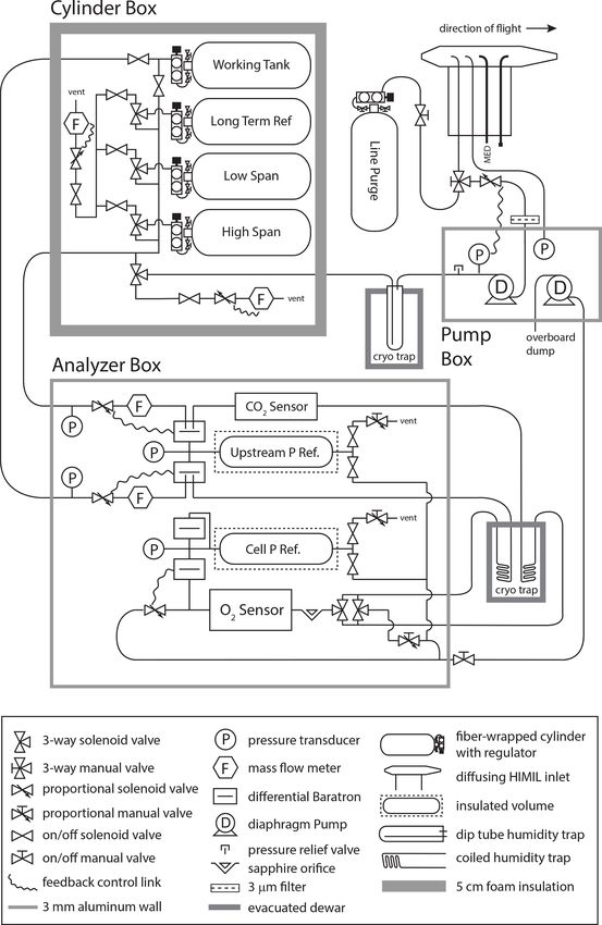
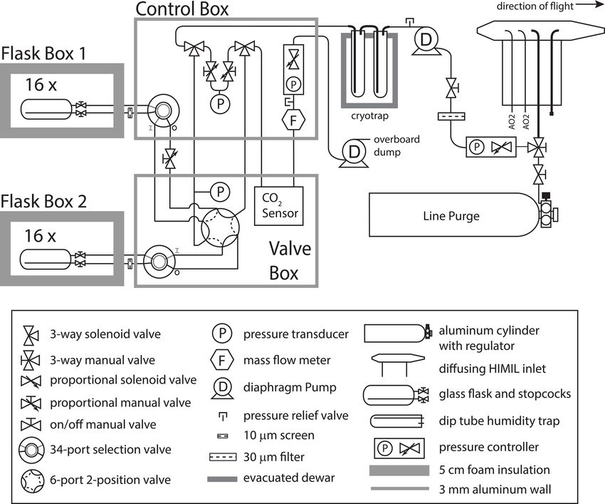
The AO2 gas handling system depicted in Fig. 1 consists of potential for fractionation in splitting the flow in the cylinder
a pump box, a cylinder box, an analyzer box, an inlet, and a box manifold. The calibration gases are contained in high-
cryotrap. See Table S1 in the Supplement for selected vendor pressure, 4.7 L fiber-wrapped aluminum cylinders, horizon-
and part numbers. We describe AO2 here in the general order tally mounted in a block of foam insulation 5 cm thick at the
of the sample air moving through the system. During ATom outside walls. Two-stage brass regulators on each calibration
2–4, AO2 sampled from an aft-facing 3.2 mm OD, 2.2 mm gas cylinder are adjusted to match the delivery pressure of
ID electropolished stainless steel inlet inside of a HIAPER the inlet sample pump during preflight, but as they are refer-
modular inlet (HIMIL) pylon 47.5 cm from the aircraft skin. enced to cabin pressure, the absolute delivery pressure of the
The HIMIL is a cigar-shaped tube with a 6.4 mm ID coni- regulators varies in flight.
cal knife edge forward inlet, a 22 mm ID cylindrical bore, The inlet line purge gas is in a similar cylinder but
and a 9.5 mm ID outlet, and is designed to slow the rela- mounted vertically outside of the insulated cylinder box and
tive air speed to minimize acceleration effects at the internal uses a similar regulator but with a lower delivery pressure
3.2 mm inlet to the instrument. The HIMIL contains the AO2 of 70 hPa above cabin. During ACME-07, prior to Research
and Medusa sample inlet tubing, an open tube connected to a Flight 10 on START-08, and during HIPPO-3, we used a
pressure sensor, and an unused sample tube. The AO2 inlet is coiled 6.4 mm diameter electropolished stainless steel mois-
the aftmost of these. Except where noted, all tubing exposed ture trap held at approximately 1 ◦ C as a preliminary drying
to sample air in AO2 is 3.2 mm OD, 2.2 mm ID electropol- stage. Out of concerns for surface effects, and because the
ished Sulfinert-treated stainless steel to minimize surface ad- aircraft spent the most time sampling very dry air, this trap
sorption and desorption effects. has not been used since (Table S2 in the Supplement).
Immediately inside the aircraft from the inlet, a manual The working tank and the selected sample or calibration
three-way valve selects air from either the inlet or a line gas, which we refer to as the span gas, are next pulled through
purge cylinder. Directly following this selection, a propor- the analyzer box by a downstream vacuum pump with suffi-
tional solenoid valve actively controls the pressure in the line cient capacity to operate the detector cell at < 100 hPa. Both
to the instrument rack and at the inlet to an upstream vacuum airstreams first pass, in sequence, an absolute pressure sen-
pump. The pump uses Teflon-coated diaphragms and Teflon sor, a proportional solenoid valve, a mass flow meter, and
valve plates sealed by o-rings to custom aluminum heads, the a 13 hPa full-scale differential pressure sensor referenced to
latter used to minimize volume. Before entering the pump a common 500 mL insulated volume maintained at 400 hPa.
box, we filter sample air using a 3 µm pore by 47 mm di- The feedback controllers for these solenoid valves actively
ameter mixed cellulose ester filter in a stainless steel holder. match this pressure to within ±1.5 Pa (1σ at 0.4 Hz). The
The feedback controller for the inlet solenoid valve is refer- span gas is then measured for CO2 by a single cell non-
enced to an absolute pressure sensor downstream of the pump dispersive infrared CO2 / H2 O sensor. We replaced the CO2
and maintains a pump outlet pressure of 1050 ± 7 hPa (1σ sensor internal plastic tubing with 3.2 mm OD stainless steel,
at 0.4 Hz) over the full range of flight altitudes. The sample but to avoid ground loops through the sensor, we inserted
air is then cryogenically dried with a 1.6 cm ID by 20.5 cm PFA union fittings inline to break electrical conductivity. The
long electropolished stainless steel trap immersed in a dry ice two streams are then cryogenically dried, the second time for
and Fluorinert slurry at −78.5 ◦ C to a depth of 18 cm at the the sample gas and as a precaution for calibration and work-
start of a flight. At the pump outlet pressure of 1050 hPa this ing tank gases, in 3.2 mm OD, 2.2 mm ID by 120 cm long
results in a saturation vapor concentration of 1.5 ppm. The coiled tubes immersed in the dry ice slurry. At 400 hPa, the
air enters the trap at the top and exits through a 3.2 mm OD, saturation vapor concentration in these traps is 3.8 ppm H2 O.
2.2 mm ID dip tube extending near the bottom of the trap. We While this is wetter than saturation for the first-stage trap and
https://doi.org/10.5194/amt-14-2543-2021 Atmos. Meas. Tech., 14, 2543–2574, 2021
2546                                                    B. B. Stephens et al.: Airborne measurements of oxygen concentration

Figure 1. Plumbing diagram of the AO2 instrument. AO2 consists of an inlet, a pump box, an insulated cylinder box, an analyzer box, a
single cryotrap shown here in two parts, and an external purge cylinder. See Sect. 2.1 for a description of the individual components. See
Table S1 in the Supplement for selected vendor and part numbers.

calibration gas, we include it because the first-stage sample          is intended to remove any of this water, and we include a trap
trap may not dry to saturation owing to residence time or dif-         on the working tank line both for consistency and as an added
fusion limitations, and the span gases may pick up a small             precaution.
amount of water permeating through the seals in the CO2                   After the coiled tube traps, the gases reach a changeover
sensor (see Sect. 4.5 below). The second-stage span gas trap           valve manifold with two rapid-switching, long-life, minia-

Atmos. Meas. Tech., 14, 2543–2574, 2021                                                  https://doi.org/10.5194/amt-14-2543-2021
B. B. Stephens et al.: Airborne measurements of oxygen concentration                                                         2547

ture three-way solenoid valves configured to work as a low-        pressure corresponds to an optical depth of 3.8, or absorp-
volume four-way changeover valve. These valves alternately         tion of 98 % of the light, and a scaling factor of 3.0 be-
select the span or working tank gas to either be measured by       tween changes in δ(O2 /N2 ) and relative changes in the signal
the VUV detector cell or vented through a bypass line. On          (1V / V). This factor differs from 3.8 because the conversion
the VUV detector line, a 0.2 mm sapphire jewel orifice im-         between relative changes in mole fraction and δ(O2 /N2 ) in-
mediately upstream of the cell acts as a critical flow orifice     cludes division by (1-XO2 ) (see Eq. 4 in Keeling et al., 1998).
and reduces the pressure to 95 hPa as it passes through the        We amplify and convert the resulting detector current of ap-
cell. A proportional solenoid valve downstream of the cell         proximately 80 nA with a low noise op amp and 1.25 × 10⁸
controls this pressure to within ±0.009 Pa (1σ at 0.4 Hz) by       ohm resistor (Stephens et al., 2003) and measure it using a
referencing a 1.3 hPa full-scale differential pressure sensor to   24-bit analogue-to-digital converter. As indicated in Fig. 2,
a second 500 mL insulated volume. Between the changeover           there is a tradeoff between absorbing more light to achieve
valve and the orifice we use 1.0 mm ID tubing to minimize          greater sensitivity and the increase in shot noise with the re-
sweepout times. A manual needle valve is located on the by-        duced number of photons reaching the detector. The current
pass line to match the combined flow impedance of the VUV          limits defined by the photocathode and op amp configuration
detector line. The flow through the instrument is nominally        are also relevant. Figure 2 also shows the typical noise from
100 sccm, set by the sapphire orifice and the upstream refer-      the instrument running calibration gas without switching in
ence pressure. Solenoid valves and pressure gauges allow the       the lab, which indicates that the detector is within a factor
reference volume pressures to be monitored and adjusted if         of 2.4 of the shot and Johnson noise limit and that the pre-
necessary between flights or for testing.                          dicted noise is not particularly sensitive to the choice of cell
   The VUV source consists of a Xe resonance lamp with a           pressure between 80 and 120 hPa.
MgF2 window powered by a 15 W 180 MHz radio frequency                 Our aircraft and lab systems also do not have the beam
oscillator, which emits strongly at 147 nm and more weakly         splitter and second detector described in Stephens et al.
at 129 nm (Okabe, 1964). The detector is a CsI photocath-          (2003) because we found that measurement noise could not
ode with a MgF2 window and peak output of 100 nA. The              be reduced by referencing to the unabsorbed beam, either
analyzer box and O2 sensor have essentially the same con-          because lamp output is not a dominant source of noise or
figuration as the shipboard instrument described in Stephens       plasma variations were imaged differently by the two detec-
(1999) and Stephens et al. (2003) with a few key differences.      tors. We correct for the imperfect control of cell pressure on
The airborne instrument, and our laboratory system, now use        short timescales using the measured pressure differential be-
a sealed Xe lamp instead of the original flow through design.      tween the cell and reference volume. We also employ a sec-
In addition to the MgF2 windows on the lamp and detector,          ond identical 1.3 hPa full-scale differential pressure sensor
we have also employed a sapphire window in front of the de-        with both ports plumbed together to correct for acceleration
tector on the aircraft instrument to eliminate the secondary       effects on the primary sensor (Fig. 1). These sensors have
Xe line at 129 nm. Earlier tests using a sapphire window           acceleration sensitivities of approximately 0.1 Pa s2 m−1 . We
fused to the lamp body with a proprietary coating, showed          orient all pressure sensors parallel to the longitudinal axis of
large humidity effects that we previously speculated might         the aircraft to minimize the impact of vertical and horizon-
have resulted from water adsorption on the sapphire coating.       tal accelerations during turbulence, but they do experience
These effects no longer appear to be as significant, either be-    changes in the longitudinal component of gravity with air-
cause of the use of an uncoated sapphire window or because         craft pitch, and longitudinal accelerations during intentional
the earlier problems may have been a result of inadequate          yaw maneuvers, or on takeoff or landing (Sect. 4.6.5).
drying. However, to further minimize concerns we place an             AO2 control and data acquisition is done by an embedded
additional MgF2 disc on the sample cell side of this sapphire      computer and analogue-to-digital converters in each box. In
disc. We also use a 1 mm thick aluminum aperture disc with         addition to the primary sensor measurements, for diagnostic
a 6.4 mm diameter hole between this MgF2 window and the            purposes, AO2 logs 16 temperatures, 12 pressures, and four
sample cell to avoid damaging the CsI photocathode with too        flows at 0.4 to 10 Hz.
much light. The VUV absorption cell is thus defined on one
side by the detector window and aperture disc and on the           2.2   Measurement approach and precision
other by the lamp window and is a 4.3 mm long by 13 mm
diameter cylinder with a 5.3 mm path length accounting for         To achieve the high levels of precision desired, AO2 switches
the aperture.                                                      between sample gas and working tank gas approximately ev-
   Figure 2 shows the relationship between detector voltage        ery 2.3 s, more than a factor of 2 faster than the earlier ship-
and cell pressure with this configuration, along with pre-         board instrument (Stephens et al., 2003). The AO2 measure-
dicted noise contributions from thermal and shot noise. Us-        ment is then based on the amplitude of the resulting square
ing sapphire to exclude the 129 nm line in a region of weaker      wave as defined by the bidirectional difference in signals be-
O2 absorption allows the instrument to be run at higher cell       tween a particular jog and an average of the prior and subse-
pressures and greater absorption factors. The 95 hPa cell          quent jogs. This yields a statistically independent measure-

https://doi.org/10.5194/amt-14-2543-2021                                             Atmos. Meas. Tech., 14, 2543–2574, 2021
2548                                                        B. B. Stephens et al.: Airborne measurements of oxygen concentration

                                                                          ods under different drying conditions. The low volume of the
                                                                          switching solenoid valves, the detector cell, and the inter-
                                                                          vening tubing, and the low cell pressure result in very fast
                                                                          cell flushing times on the order of 0.02 s. The instrument
                                                                          records a number of housekeeping signals over the first 0.3 s
                                                                          after switching and by the time it records the VUV detec-
                                                                          tor signal again the cell has almost completely swept out.
                                                                          As a result, artifacts due to incomplete sweepout are small.
                                                                          The difference in slopes between the working tank and span
                                                                          segments of the square wave is only marginally influenced
                                                                          by the magnitude of the difference in concentration between
                                                                          the two gases, and we do not exclude any data following the
                                                                          changeover valve switch. However, the slope difference be-
                                                                          tween working tank and span segments can provide an im-
                                                                          portant diagnostic of several other possible issues, including
                                                                          delays in pressure equilibration from small cross-port leaks
                                                                          in the changeover valve or differences in humidity or hy-
                                                                          drocarbons leading to chemical interactions with optical sur-
                                                                          faces under intense VUV (see Sect. 4.5 below).
                                                                             Atmospheric oxygen is quantified as the ratio of the rela-
                                                                          tive abundance of O2 to the relative abundance of N2 in units
                                                                          of per meg (Keeling and Shertz, 1992; Keeling and Manning,
                                                                          2014), i.e.,

                                                                                          (O2 /N2 )sample
                                                                          δ(O2 /N2 ) =                    − 1 × 10⁶ ,                (1)
                                                                                            (O2 /N2 )ref
                                                                          where 1 per meg represents a one-millionth change in the
                                                                          O2 /N2 ratio relative to an arbitrary reference. For the Scripps
                                                                          O2 Program O2 scale, this reference is a suite of high-
                                                                          pressure cylinders maintained at Scripps. An analogous defi-
                                                                          nition to Eq. (1) is used to report measurements of the Ar/N2
                                                                          ratio. In addition to δ(O2 /N2 ) and CO2 , we also report values
                                                                          for the derived tracer atmospheric potential oxygen (APO;
Figure 2. Typical results from a pressure scan of the AO2 detec-
                                                                          Stephens et al., 1998):
tor cell showing (a) the logarithmic relationship between detector
volts and cell pressure as well as current limits for the amplifier and                          1.1
photocathode. Owing to sensitive tuning of the cell pressure con-         APO = δ(O2 /N2 ) +         (CO2 − 350),                       (2)
                                                                                                 XO2
trol system in this configuration, control above 140 hPa is unstable.
The values in (a) give the unattenuated lamp signal and apparent          where 1.1 is the estimated stoichiometric ratio of long-term
absorption coefficient defined by the y intercept and slope of the fit.   terrestrial biosphere O2 and CO2 exchange, and XO2 is the
Using these values, (b) shows predicted noise contributions to com-       mole fraction of O2 in dry air as defined by the Scripps
parisons of subsequent 2 s averages from shot and Johnson noise as        O2 Program O2 scale. APO is designed to be conservative
well as the Beer’s law scaling between relative changes in δ(O2 /N2 )     with respect to terrestrial photosynthesis and respiration, to
and detector output and the resulting predicted noise in δ(O2 /N2 ).      only have a small fossil-fuel sink, and to primarily reflect
The single point in (b) corresponds to typical performance while          δ(O2 /N2 ) and CO2 exchange with the oceans. Although 1.05
running calibration gas either directly or through a trap at room
                                                                          is likely a better O2 : CO2 ratio for canceling short-term ter-
temperature (Sect. 2.2). There is little change and no minimum in
predicted noise over the pressure range shown.
                                                                          restrial influences (Stephens et al., 2007a; Battle et al., 2019),
                                                                          we continue to use 1.1 here for consistency with past stud-
                                                                          ies and encourage sensitivity tests over a range of possible
                                                                          O2 : CO2 ratios.
ment every 4.6 s (hereafter rounded to 5 s), though we report                Figure 4 shows instrument noise as a function of hypo-
partially overlapping differences every 2.3 s. The switching              thetical switching time based on 40 min of calibration gas
time is set by the amount of time the instrument needs to                 analysis with no actual valve switching in the lab. This figure
record 20 detector voltages at 10 Hz and then housekeeping                includes the two-sample Allan standard deviation, as well as
variables between switches. Figure 3 shows the 5 s square                 the standard deviation of the bidirectional three-sample dif-
wave signal averaged over the calibration and sample peri-                ferences we use, the latter of which has a broad minimum

Atmos. Meas. Tech., 14, 2543–2574, 2021                                                     https://doi.org/10.5194/amt-14-2543-2021
B. B. Stephens et al.: Airborne measurements of oxygen concentration                                                               2549

                                                                          We find similar noise levels whether switching or not
                                                                       switching the changeover valve between working tank and a
                                                                       calibration gas, or between working tank and span gas when
                                                                       the trap is warm, indicating that pressure and flow fluctua-
                                                                       tions from the actual switching do not add noise. Rather, the
                                                                       slight increase in noise for calibration gases in flight rela-
                                                                       tive to lab conditions is likely a result of aircraft motion and
                                                                       slight drift within the flight calibration intervals. However,
                                                                       the switching of the changeover valve does introduce extra
                                                                       noise when running either long-term surveillance gas or sam-
                                                                       ple air through the first-stage trap when it is cold, suggest-
                                                                       ing an interaction between flow perturbations and thermal
                                                                       diffusion in the trap (Keeling et al., 1998). Thus, our typi-
                                                                       cally achieved precision when measuring ambient air in sta-
                                                                       ble conditions is 2.5–4.0 per meg, 1σ in 5 s. Figure 5 shows
                                                                       O2 and CO2 signals over the course of an entire flight, includ-
                                                                       ing several hours of preflight and 15 min of postflight inlet
                                                                       line purge analysis. For the 36 min high altitude period be-
                                                                       tween 22:23 and 23:00 in Fig. 5, the variability in δ(O2 /N2 )
                                                                       is ±3.5 per meg (1σ for 5 s samples) and as low as ±2.5
Figure 3. Average AO2 square wave shapes from a high-span (HS)         per meg for similar periods on other flights (e.g., Fig. S3 in
calibration period (a, c) and sample (SA) gas period (b, d) from
                                                                       the Supplement). For comparison, 2.5 per meg is equal to a
an example ATom-3 flight (a, b) and an example HIPPO-5 flight
(c, d). Points are calculated as the median VUV signal binned by
                                                                       change of 0.4 ppm in O2 mole fraction or the addition of 0.5
jog position over multiple jogs, as indicated by the n value in each   micromoles of O2 to 1 mole of air (Keeling et al., 1998; Ko-
panel, and plotted relative to the average working tank (WT) sig-      zlova et al., 2008). This variability averages as white noise
nal. Dashed vertical lines indicate the times when the four-way        and with statistically independent samples every 5 s, the pre-
changeover valve switched. The gaps after switching correspond to      cision on a 1 min average is approximately ±0.7–1.1 per meg
the system logging less frequent diagnostic signals, and no points     while measuring ambient air and 0.4 per meg for calibration
have been removed during the transitions. The right y axes show the    gas.
raw VUV signal in mV and the left y axes show approximate per
meg δ(O2 /N2 ). Slopes of the individual span and working tank seg-    2.3   In-flight calibration strategy
ments are also reported in units of per meg s−1 in each half panel.
The difference between span gas and working tank slopes is only
                                                                       The AO2 high-pressure reference cylinders are equipped
−1 to −2 per meg s−1 in the ATom-3 examples but −20 to −30 in
the HIPPO-5 panels, which we attribute to inadequate drying (see
                                                                       with brass valve manifolds sealed with silver-coated c-rings.
Sect. 4.5).                                                            These manifolds have needle valves going to either a fill and
                                                                       laboratory analysis port or a regulator for use in flight, a burst
                                                                       disc, and a 20 cm dip tube to minimize thermal fractionation
of 1.25 per meg between simulated switching times of 2 and             in withdrawn air (Keeling et al., 2007). These dip tubes were
3 s. The slope of the rise in noise for shorter intervals sug-         one of 6.4 mm OD, 4.6 mm ID stainless steel; 3.2 mm OD,
gests that there would be no improvement from switching                1.4 mm ID nickel; or 0.16 mm OD, 1.0 mm ID electroformed
faster. Figure 4 also shows typical noise values from the in-          nickel supported by a perforated 6.4 mm stainless steel tube.
strument while running calibration gas with switching and              We fill these cylinders to 200 bar with ambient air from larger
while measuring ambient air with stable concentration, both            cylinders filled by NOAA/GML at Niwot Ridge, CO. We
during field conditions. Although at times AO2 noise while             then adjust the O2 and CO2 concentrations in these cylin-
running calibration gas is 1.25 per meg or better (1σ in 5 s),         ders and calibrate them against laboratory references trace-
the value shown here of 1.6 per meg is more consistently               able to both the Scripps O2 Program O2 scale, as defined on
achievable. For example, the median of the 5 s noise levels            16 March 2020, and the WMO X2007 CO2 scale. We mea-
within all individual calibration gas intervals was 1.5 per meg        sure each flight cylinder in the lab over a period of several
for ATom-3, and 1.7 for ATom-4. Our correction of imperfect            weeks both before and after a field deployment to detect and
cell pressure control based on the downstream 1.3 hPa differ-          account for any drift (Sect. 4.6.1).
ential pressure sensor has a negligible effect for the lab con-           Approximately every 50 min during flight, we measure the
ditions shown in Fig. 4 but can reduce the noise in turbulent          high- and low-span cylinders for 2.5 min each, alternating
flight conditions by a factor of 5 or more.                            their order each time to detect any flushing issues (Fig. 5).
                                                                       We measure the working tank against itself for 2.5 min for an
                                                                       additional CO2 calibration point every other calibration cy-

https://doi.org/10.5194/amt-14-2543-2021                                                 Atmos. Meas. Tech., 14, 2543–2574, 2021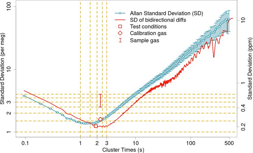
2550                                                      B. B. Stephens et al.: Airborne measurements of oxygen concentration

Figure 4. AO2 signal noise characteristics from a laboratory test running a single calibration gas without changeover valve switching for
40 min on a log–log plot. The two-sample Allan standard deviation and errors are as calculated by the allanvar package in R. The standard
deviation of the three-sample bidirectional differences are calculated as in AO2 processing for hypothetical valve switching intervals. During
this test the instrument was able to make 20 analog to digital conversions in 1.9 s rather than 2.3 s as in flight, owing to sampling fewer
diagnostic signals. Symbols show the results of applying the AO2 processing on 20-sample intervals from this lab test, as well as a more
typical value for calibration gas during smooth flight conditions and a typical range of values for sample gas in flight during smooth to
moderate turbulent conditions. The increase in noise for calibration gas in flight is related to slight motion effects and trends during a
calibration cycle. The increase in noise for sample air in smooth flight is likely caused by thermal gradients in the cryotrap. The left y axis
shows values in per meg δ(O2 /N2 ) and the right y axis shows ppm in O2 mole fraction.

cle and we measure the long-term reference for 2.5 min as a               2.4   Data processing
system diagnostic every third calibration cycle. Before each
calibration gas is measured, we purge it at our sample flow               Similar to the processing of shipboard data described in
of 100 mL min−1 for 2.5 min. We exclude 60 s of data after                Stephens et al. (2003), the amplitude of the 5 s switching sig-
every switch to a calibration gas or back to sample and aver-             nal is proportional to the mole fraction of O2 in the sample
age the remaining data for each calibration period. Allowing              gas and forms the basis of the AO2 measurement (Fig. 5). For
for these transitions, a two-point calibration excludes 6 min             O2 , we calculate a linear fit for each paired high-span–low-
of ambient air measurement and a four-point calibration ex-               span calibration cycle to apparent mole fraction (Stephens
cludes 11 min.                                                            et al., 2003) and interpolate these fit parameters linearly in
   Starting with HIPPO-3, we added a fifth cylinder of air                time to ambient air or long-term reference measurements.
to purge the inlet line during pre- and postflight periods to             For CO2 , we first calculate a quadratic fit to calibration cycles
prevent ingesting aircraft exhaust and to dry inlet lines dur-            that also include the working tank gas and interpolate and ap-
ing preflight (Sects. 4.3 and 4.5). Starting with ORCAS, we               ply these parameters to cycles with only high-span and low-
also used this purge air to flush and dry inlet tubing during             span gases before calculating secondary linear fits for these
maintenance days. This cylinder is mounted vertically and                 cycles and interpolating to sample and long-term reference
external to the insulated cylinder box. We load dry ice in the            measurements. After calculating apparent mole fractions of
dewar approximately 2.5 h before takeoff and then start the               O2 for the entire flight, we convert these to δ(O2 /N2 ) and
working tank and inlet line purge gases flowing and turn on               correct for dilution using the concurrent calibrated measure-
the VUV lamp 2 h before takeoff to warm up and dry out the                ments of CO2 (see Eq. 4 in Stephens et al., 2003). After the
instrument. During the hour immediately before takeoff, we                preflight period, the O2 calibration as defined by the linear fit
run our calibration sequence four times at 15 min intervals to            to high- and low-span cylinder measurements is very stable,
flush the regulators and dry out the calibration manifold and             with typical drift rates of less than 5 per meg per hour and
tubing.                                                                   less than 15 per meg over an 8–10 h flight. For Fig. 5, the
                                                                          standard deviation of the 13 in-flight high-span calibration
                                                                          gas measurements is ±2.5 per meg.

Atmos. Meas. Tech., 14, 2543–2574, 2021                                                      https://doi.org/10.5194/amt-14-2543-2021
B. B. Stephens et al.: Airborne measurements of oxygen concentration 2551
Figure 5. AO2 CO2 and O2 signals from ATom-4 Research Flight 2, from Palmdale, California, to Anchorage, Alaska, with profiles over the
northeast Pacific and Arctic oceans. CO2 signals are from the internal Li-820 sensor and O2 signals are the amplitude of the 5 s square wave,
converted to approximate ppm and per meg using a single linear calibration for the entire flight for each species. The calibration intervals
include the last 1 h 15 min of preflight with line purge gas on the sample line and calibration cycles every 15 min, in-flight calibrations
nominally spaced by 50 min, and 15 min of postflight line purge and a final calibration cycle. The anticorrelated vertical gradients in CO2
and O2 are consistent with buildup of industrial emissions and respiration over winter and late spring.
We shift our measurements in time using inlet lags em- two external pumps, an inlet, a purge cylinder, and a stain-
pirically determined from the switches to and from inlet line less steel dewar. See Table S1 in the Supplement for selected
purge cylinder gas before and after each flight, plus a minor vendor and part numbers. Medusa shares the same HIMIL
additional pressure-dependent lag for the remaining portion pylon with AO2 but samples from a 6.4 mm OD, 4.6 mm ID
of the inlet upstream of this valve. At our present sample aft-facing electropolished stainless steel inlet tube, which is
flow rate and trap volume, the total inlet lag is approximately in the second position behind a fourth unused inlet tube of
50 s with a ±10 s smoothing window attributable to shear and the same size. Air is drawn from the inlet into the system
turbulence induced mixing in the tubing and traps. This lag by an upstream vacuum pump modified in the same way as
time was 10 s shorter with the small diameter trap used prior for AO2, while a pressure controller located immediately in-
to ARISTO-2015 and varied by a similar amount, owing to side the aircraft maintains a constant pressure upstream of
differences in flow and inlet lengths across campaigns. the pump. Similar to AO2, between the inlet and this first
On specific flights and campaigns, we make additional cor- control valve, a manual three-way valve allows the system
rections to the AO2 data as described in Sects. 4.2, 4.3, 4.4, to sample from a purge gas cylinder containing dried natu-
and 4.5. ral air. In the case of Medusa, this inlet purge cylinder was
added prior to ORCAS. Between the pressure controller and
the pump, the sample air is filtered by a 30 µm pore by 47 mm
3 NCAR/Scripps Medusa Flask Sampler diameter polypropylene filter in a stainless steel holder. After
passing through the upstream pump, the sample air is dried in
3.1 Sampler description series by two 2.2 cm ID by 23 cm long electropolished stain-
less steel traps immersed in a similar dry ice and Fluorinert
The Medusa gas handling system is shown in Fig. 6. Medusa slurry as for AO2. We use 3 mm glass beads in the lower
consists of two identical insulated flask boxes, each of which 10 cm of these traps, resulting in approximate trap volumes
holds 16 flasks, a control box that houses most of the pres- of 54 mL. We actively heat the inlet to the upstream trap to
sure control system and the system computer, a valve box a temperature of 4.5 ◦ C to prevent water freezing out before
that holds two additional multi-position gas handling valves,
https://doi.org/10.5194/amt-14-2543-2021 Atmos. Meas. Tech., 14, 2543–2574, 20212552 B. B. Stephens et al.: Airborne measurements of oxygen concentration reaching the trap itself and obstructing flow. When the ambi- purge cylinder air. Before sampling, we flush the flasks with ent dew point is greater than 4.5 ◦ C, water will start to con- a minimum of 5 volumes of sample air before moving to the dense at this location, but as it is only several centimeters next position. At the time of sample collection, the system directly above the trap, we expect any formed drops to mi- temporarily switches flow to a bypass loop with matched grate into the cold trap. The dried air is then directed to the impedance, while a rotary valve isolates the air within the inlet of one of the 32 flasks by a series of rotary multiposi- sampled flask and connecting tubing. At a later time, nomi- tion valves. A second pump and pressure controller down- nally several minutes to an hour, the onboard operator man- stream of the flask outlets controls flask pressure to approxi- ually closes the flask stopcocks to preserve the sample. We mately 1 atm. Medusa includes a single-cell CO2 / H2 O sen- record system pressures, flows, and diagnostic CO2 and H2 O sor downstream of the flasks to provide diagnostics of flask at 1 Hz. After each flight we disconnect and remove the up- drying and mixing, and detection of potential cabin-air leaks. stream trap, using normally closed quick connect fittings. All Medusa tubing is electropolished 6.4 mm OD, 4.6 mm During maintenance days, we exchange flasks, install a dry ID stainless steel or flexible ethylene copolymer lined tub- upstream cryotrap, and pressure test all connections for leaks. ing. Flexible tubing includes approximately 50 cm of flexible lines of 6.4 mm OD, 4.3 mm ID upstream and downstream 3.2 Flask analysis of each flask; approximately 1 m lines of the same intercon- necting the valve and control boxes; and 60 cm of 9.5 mm Sampled flasks are shipped to Scripps Institution of OD, 6.4 mm ID upstream of the first pump to reduce intake Oceanography for analysis. We try to minimize the tem- impedance. Medusa collects air samples into 1.5 L (30 cm perature range to which flasks are exposed before analysis, long by 8 cm diameter) borosilicate glass flasks that are con- but this is not always possible and hence flasks can be ex- tained within a block of foam insulation 3 cm thick at the posed to a variety of environments before they reach the outside walls, with the stopcocks and tubing connections pro- lab. Flasks are typically analyzed within 3 months of col- truding from the foam. The sample air enters the flask at the lection, with a median storage time for all flasks of 80 d. exposed end and exits the flasks via a 24 cm dip tube extend- The flask analysis includes measurements of CO2 on a non- ing into the flask with the intent to minimize thermal fraction- dispersive infrared analyzer (LI-COR 6252) and of δ(O2 /N2 ) ation effects and improve flushing (see Sect. 4.1). The stop- and δ(Ar/N2 ) on a sector-magnet mass spectrometer (Mi- cocks use Viton o-rings lightly coated with vacuum grease cromass IsoPrime; Keeling et al., 2004), followed by ex- to minimize permeation effects and flask breakage (Keeling tracting CO2 for subsequent isotopologue measurements. We et al., 1998). do not find any evidence of storage effects in δ(O2 /N2 ), Pressure sensors on the bypass line and immediately up- δ(Ar/N2 ), or CO2 over these timescales. We measure the ex- stream of the first multi-position valve and a manual propor- tracted CO2 for 13 C and 18 O on an Optima mass spectrom- tional valve between the valve and control boxes allow for eter (Guenther et al., 2001) and recapture and preserve the balancing and monitoring system pressures. A manual on/off CO2 for eventual measurement of 14 C. The single-flask 1σ valve on the inlet line facilitates leak checking. The return precision for the δ(O2 /N2 ) and CO2 measurements are ±3 lines from each flask include 10 µm stainless steel screens to per meg and ±0.15 ppm, respectively (Keeling et al., 2004). protect the multi-position valves from the potential introduc- The CO2 , δ(O2 /N2 ) and δ(Ar/N2 ) measurements are done tion of foreign debris during flask swapping. The flow rate by first withdrawing 150 mL of air over 5 min out of the flask through the system is set by the upstream and downstream while replacing this lost volume with a purge gas with known pressure set points, selected from a range of predetermined concentrations and artificially low CO2 . The flasks are con- options to maximize flow while maintaining approximately tained in an insulated box during analysis to minimize tem- 1 atm in the flask and the upstream controller pressure set perature fluctuations. If the flasks are to be measured subse- point below ambient. At the maximum altitudes of the GV quently for stable carbon isotopes, we correct for the dilu- and DC-8, we typically use an upstream set point of 146 hPa tion with purge gas by remeasuring the CO2 content after the with a flow rate of approximately 1550 mL min−1 and at flasks have equilibrated overnight (Kort et al., 2008; Bent, the lowest altitudes we typically use an upstream set point 2014). This second CO2 analysis is done on a 90 mL sub- of 226 hPa, which produces a flow rate of approximately sample without replacement. We extract all remaining CO2 2700 mL min−1 . After switching between pressure settings, for the 13 C, 18 O, and 14 C measurements. we allow 10 min for the system to stabilize before sampling Calibration gases for the mass spectrometer are introduced when switching to the lowest flow and 5 min when switching from the laboratory interferometer system via a tee and we to the highest flow. correct the Medusa flask measurements for empirically deter- Before each campaign, we purge the flasks in the labo- mined offsets owing to fractionation at this tee of +6.4 and ratory with 5 volumes of cryogenically dried cylinder air at +8.5 per meg for δ(O2 /N2 ) and δ(Ar/N2 ), respectively. The ambient CO2 and O2 levels and store them with an internal direction of flow during analysis is in through the dip tube to pressure of 1 atm. Then, before each flight, we purge them be consistent with Scripps O2 Program network flasks. The for 1 min on the high flow setting in the sampler with line flasks are mounted horizontally during analysis with half of Atmos. Meas. Tech., 14, 2543–2574, 2021 https://doi.org/10.5194/amt-14-2543-2021
B. B. Stephens et al.: Airborne measurements of oxygen concentration                                                                 2553

Figure 6. Plumbing diagram of the Medusa flask sampler. Medusa consists of an inlet, a control box, a valve box, two insulated flask boxes,
a cryotrap, two pumps, and a purge cylinder. See Sect. 3.1 for a description of the individual components. See Table S1 in the Supplement
for selected vendor and part numbers.

the flasks having their dip tubes upwards and the other half            where w(t) is the weighting of any 1 s time increment t be-
rotated 180 degrees with their dip tubes downwards. We are              tween the switch to the sampled flask and the switch to the
able to detect gravitational fractionation effects during anal-         next flask, tf , and τ is the flushing time in seconds, i.e., the
ysis with flasks with lower outlets having enhanced concen-             flask volume divided by the mean flow during the sampling
trations of the heavier species and vice versa. We apply em-            period. w(t) is scaled so that it sums to 1 for all non-missing
pirical corrections for this effect of ±0.8 and ±2.4 per meg            values over a given sampling interval. These weighting ker-
for δ(O2 /N2 ) and δ(Ar/N2 ), respectively.                             nels are reported along with the final Medusa data.
                                                                           Despite careful attention in the field and lab, it is possi-
3.3   Data processing                                                   ble for flasks to experience leaks during the various stages of
                                                                        sampling, shipping, storage, and analysis. The analysis sys-
Laboratory tests indicate that mixing of air in the flasks dur-         tem at Scripps has automated checks to reject flasks with
ing sampling is well approximated by an e-folding time equal            obvious anomalies in fill pressure or other parameters. In
to the flask volume divided by the flow rate. The characteris-          addition, we manually identify and flag flasks with CO2 ,
tic mixing time for the Medusa flasks is approximately 33 s at          δ(O2 /N2 ), and δ(Ar/N2 ) measurements well out of range of
the highest flow rate and 60 s at the lowest flow rate. We es-          expectations from the concurrent CO2 measurements made
timate the combined inlet and cold trap lag time for Medusa             by AO2 and other instruments, δ(O2 /N2 ) from AO2, and
from volume/flow to be 7 s at the highest flow setting and              background δ(Ar/N2 ) values. Of the 4004 flasks sampled in
13 s at the lowest flow setting. To compare the flask measure-          the 12 most recent campaigns, 209 were flagged during anal-
ments to state parameters and other chemical measurements               ysis at Scripps and an additional 109 were manually flagged
sampled at higher frequency, we use a weighting kernel for              after analysis.
each flask that is based upon the measured flow rate, tub-                 All flask measurements are referenced to a hierarchy of
ing lags, and sampling start and end times (Kort et al., 2008;          calibration cylinders to measure them on the Scripps O2 Pro-
Bent, 2014):                                                            gram O2 and CO2 scales (Keeling et al., 1998, 2007). The
                                                                        NCAR primary cylinders, measured both by Scripps and
            tf −t
                                                                       NOAA, allow us to establish a link between the Scripps O2
w(t) = e−     τ         ,                                      (3)

https://doi.org/10.5194/amt-14-2543-2021                                                   Atmos. Meas. Tech., 14, 2543–2574, 2021
2554 B. B. Stephens et al.: Airborne measurements of oxygen concentration
Program CO2 scale and the WMO CO2 scale in order to re- pected slopes for thermal and pressure fractionation of flask
port the flask measurements on the WMO scale in campaign samples at 1 atm (Keeling et al., 2004). Except in the lower
merge products and to use common scales in comparison stratosphere, we expect only small changes in δ(Ar/N2 ) and
with AO2 measurements. with slopes versus APO less than 2, so we use this figure to
rule out large effects. Figure S6 in the Supplement similarly
shows Medusa flask δ(Ar/N2 ) versus normalized Medusa–
4 Discussion of potential sources of bias AO2 APO differences, which we expect to be a more sensi-
tive indicator of fractionation. The sign of the tropospheric
Making measurements at the 10−6 relative level is challeng- Medusa δ(Ar/N2 ) versus Medusa–AO2 APO difference re-
ing and the developments of AO2 and Medusa have included lationship during START-08, HIPPO, and ORCAS on the
discovering and resolving a series of potential measurement GV suggest a fractionation effect on Medusa samples. Other
artifacts, as described in the sections below. While we now evidence of much larger inlet fractionation for AO2 than
have established practices to eliminate or minimize all of Medusa (Sect. 4.2) suggests this is less likely an inlet ef-
these effects, in some cases it has been necessary to de- fect and more likely a flask sampling effect. Though some
velop empirical corrections for recognized systematic biases. of the larger δ(Ar/N2 ) excursions are correlated with APO
The most significant of these effects have been those as- in Fig. S5 in the Supplement, the Medusa–AO2 APO differ-
sociated with inlet fractionation (Sect. 4.2) and inadequate ences and N2 O values in Fig. S6 in the Supplement suggest
drying of AO2 sample air (Sect. 4.5). We have also iden- these are of natural stratospheric origin (Birner et al., 2020).
tified subtler effects associated with thermal fractionation in Although we cannot exclude a contribution from pressure-
Medusa flasks (Sect. 4.1), regulator and tubing surface condi- driven fractionation, because pressures are actively con-
tioning (Sect. 4.3), and systematic differences between mea- trolled and more consistent during sampling, we conclude
surements on climbs and descents (Sect. 4.4). When neces- that thermal gradients in the flasks are the most likely cause
sary, we calculate adjustments for bias effects as described in of this scatter. During HIPPO, δ(Ar/N2 ) scatter was greater
Sects. 4.1.1, 4.2.1, 4.3.1, 4.4.1, and 4.5.1. We discuss other for flasks collected in the lower Medusa box closer to the GV
potential sources of bias that have fortunately not required cabin air vents. These flasks also had lower mean δ(Ar/N2 )
any adjustments in Sect. 4.6 and independent checks on mea- values (Bent, 2014). If this were a thermal fractionation ef-
surement bias in Sect. 4.7. In all reported AO2 and Medusa fect, it could result from the flask dip tube being cold in com-
data products we include both the raw and adjusted measure- parison to the surrounding flask air. On the DC-8 during the
ments to support assessment of their impacts on various con- ATom campaigns, when the Medusa rack was inboard and
clusions and use of the unadjusted data when that is more away from any air conditioning vents, the δ(Ar/N2 ) scatter
appropriate. was reduced by a factor of 2 (Figs. S4, S5, and S6 in the
Supplement) and the lower box difference was eliminated.
4.1 Fractionation of flask samples On the GV during ORCAS, we added a metal plate to the
side of the rack to partially block the cold cabin air vents and
Thermal or pressure-driven diffusive gradients can play a the δ(Ar/N2 ) scatter was reduced, but the lower box still had
role in separating Ar, O2 , and N2 under various conditions a low bias. Also, during START-08 and HIPPO-1 we con-
(Keeling et al., 1998). This is a concern for flask sampling nected half of the flasks with flow into rather than out of the
if temperature gradients exist at the point where molecules dip tubes and these flasks showed greater scatter in δ(Ar/N2 ).
are committed to exiting the flask, e.g., at the dip tube tip It is also possible that the use of the Medusa inlet line purge
when flowing out through the dip tube or at the stopcock cylinder starting with ORCAS contributed to the reduction in
if flowing in through the dip tube. Figure S4 in the Sup- δ(Ar/N2 ) scatter during ORCAS and ATom by reducing sur-
plement shows vertical profiles of δ(Ar/N2 ) measurements face effects associated with drying of tubing early in flight.
on Medusa flasks from all campaigns. Observed decreases in We have examined the dependency of δ(Ar/N2 ) on the length
δ(Ar/N2 ) in the stratosphere are consistent with estimates of of time between isolating a flask with the rotary valve and
gravitational diffusion (Ishidoya et al., 2008, 2013b; Bent, manually closing the stopcocks and do not find any rela-
2014; Birner et al., 2020; Jin et al., 2021), but we expect tionship, suggesting fractionation is not occurring during this
vertical δ(Ar/N2 ) gradients in the troposphere to be constant time.
within a few per meg (Bent, 2014). During HIPPO, the tro-
pospheric δ(Ar/N2 ) scatter about the campaign mean vertical 4.1.1 Adjustments for thermal fractionation
gradient of approximately ±20 per meg (1σ ) is considerably
larger than the synoptic or spatial variations observed at sur- We correct the Medusa δ(O2 /N2 ) measurements for appar-
face stations (Keeling et al., 2004) and we attribute most of ent thermal fractionation effects by adjusting the measured
this to fractionation at the flask outlets during sampling. Fig- δ(O2 /N2 ) values according to the expected relationship with
ure S5 in the Supplement shows Medusa flask δ(Ar/N2 ) ver- δ(Ar/N2 ) for thermal fractionation and report both original
sus APO for each campaign along with reference lines for ex- and corrected values. This correction is similar to that done
Atmos. Meas. Tech., 14, 2543–2574, 2021 https://doi.org/10.5194/amt-14-2543-2021B. B. Stephens et al.: Airborne measurements of oxygen concentration 2555
in previous studies (Battle et al., 2006; Steinbach, 2010; Ishi- 4.2 Inlet fractionation
doya et al., 2014; Bent, 2014). We use a constant reference
value of 15 per meg δ(Ar/N2 ) in the troposphere, which is Pressure gradients also have the potential to diffusively sepa-
the approximate global surface annual mean from the Scripps rate O2 and Ar relative to N2 at aircraft inlets (Keeling et al.,
O2 Program network (Table S3 in the Supplement). In the 1998). Steinbach (2010) proposed a model for aircraft inlet
stratosphere, we adjust this reference δ(Ar/N2 ) value by a fractionation resulting from pressure gradients perpendicu-
linear fit between δ(Ar/N2 ) and detrended N2 O, a proxy lar to streamlines at the inlet, whereby forward-facing inlets
for age of air, with an intercept at the tropopause transition would preferentially sample heavier molecules at high air-
(Bent, 2014). We use N2 O measurements from the Harvard craft velocity and vice versa for aft-facing inlets. We expect
Quantum Cascade Laser Spectrometer (QCLS, Santoni et al., diffusive fractionation effects to be greater by a factor of 3
2014) and the NOAA PAN and Trace Hydrohalocarbon Ex- for δ(Ar/N2 ) than for δ(O2 /N2 ) because of the greater mass
peRiment (PANTHER, ATom-1 only) instruments. The cor- difference (Keeling et al., 1998, 2004). Aircraft inlet frac-
rected δ(O2 /N2 ) values are then defined as tionation will likely also be dependent on other factors such
as ambient pressure, ram pressure, inlet shape, inlet flow rate,
δ(Ar/N2 ) − δ(Ar/N2 )ref inlet tubing wall thickness, and angle of attack. We assessed
δ(O2 /N2 )∗ = δ(O2 /N2 ) − (4)
3.77 these effects with several different configurations of aircraft
and inlet design, starting with COBRA test flights in 1999.
and by extension These have included sampling at variable speeds, angles of
attack, and flow rates, and switching between aft and for-
ward inlets during stable flight conditions. These tests for
1.1 COBRA using a forward-facing 9.5 mm inlet tube, during the
APO∗ = δ(O2 /N2 )∗ + (CO2 − 350), (5)
XO2 IDEAS campaign switching between forward and aft 3.2 and
6.4 mm diameter inlet tubes, and for START-08 or HIPPO us-
establishing new tracers, δ(O2 /N2 )∗ and APO∗ , that are ing a HIMIL, were inconclusive. However, vertical gradients
largely insensitive to thermally induced fractionation of flask in δ(Ar/N2 ) (Fig. S4 in the Supplement) and in AO2–Medusa
samples. δ(O2 /N2 ) differences (Fig. 8) do suggest non-negligible in-
This approach also corrects for any thermal fractionation let fractionation for the HIMIL. Furthermore, when using
effects during analysis, which would be indistinguishable aft and side-facing non-diffusing inlets during ORCAS and
from those during sampling. Adjusting to a constant tro- ATom-1, we observed much more dramatic fractionation ef-
pospheric vertical profile in δ(Ar/N2 ) also mostly compen- fects.
sates for potential inlet fractionation effects as discussed in One-dimensional model calculations of the balance be-
Sect. 4.2. Figure 7 shows the vertical distribution of the orig- tween gravitational separation and tropospheric mixing sug-
inal δ(O2 /N2 ) and corrected δ(O2 /N2 )∗ values from Medusa gest the mean vertical distribution of δ(Ar/N2 ) should be
flasks during all campaigns. The median δ(Ar/N2 ) offset constant to within 2 per meg below 9 km (Bent, 2014).
from the combined tropospheric value and stratospheric N2 O Furthermore, marine boundary layer seasonal variations in
relationship was −8.3±26.4 per meg (1σ ), resulting in a me- δ(Ar/N2 ) are relatively small at 10–20 per meg amplitude
dian adjustment to Medusa δ(O2 /N2 ) of +2.2 ± 7.0 per meg. (Keeling et al., 2004) and would lead to vertical gradients
For the three campaigns ATom 2–4, the median δ(O2 /N2 ) of opposite sign in different seasons. We suspect the consis-
adjustments are +1.9 ± 3.6 per meg (Table S3 in the Supple- tently observed tropospheric δ(Ar/N2 ) gradients of approxi-
ment). mately −2 per meg km−1 for the HIPPO campaigns and +2
This method of correcting for δ(O2 /N2 ) fractionation ef- per meg km−1 for ATom-1 shown in Fig. S4 in the Supple-
fects using δ(Ar/N2 ) ignores the real boundary-layer sea- ment resulted from inlet fractionation. The sign of the HIPPO
sonal cycles in δ(Ar/N2 ) of up to ±10 per meg amplitude and gradients combined with the greater relative air speeds at
likely annual mean meridional δ(Ar/N2 ) gradients on the or- higher altitude suggest preferential sampling of lighter N2
der of 5 per meg (Keeling et al., 2004; Battle et al., 2003; molecules at the aft-facing tube inside the HIMIL rather than
Bent, 2014). Thus, scientific applications of Ar-corrected at the forward-facing entrance to the HIMIL. The relative
Medusa data, or of versions of AO2 data that are adjusted airspeed inside the diffusing HIMIL pylon is considerably
based upon comparison to Ar-corrected Medusa data, need slower than outside and the flow is laminar.
to consider these additional influences. For example, Bent Motivated by concerns over the potential for cabin air to
(2014) removed the estimated contribution of seasonal Ar contaminate the sample stream through outward leaks more
variations to APO∗ from AO2 in an analysis of Southern forward on the aircraft (Sect. 4.6.3), during ARISTO-2015
Ocean O2 exchange and Resplandy et al. (2016) used lat- we evaluated a new fin HIMIL inlet design consisting of aft-
itudinal gradients of APO from AO2 adjusted to non-Ar- facing 7.9 mm OD, 6.5 mm ID tubes extending 40 cm from
corrected Medusa data in order to constrain interhemispheric the fuselage supported by (and with all but 5 mm contained
ocean heat exchange. within) a fin-shaped aerodynamic pylon. ARISTO-2015 was
https://doi.org/10.5194/amt-14-2543-2021 Atmos. Meas. Tech., 14, 2543–2574, 2021You can also read