Improved representation of the global dust cycle using observational constraints on dust properties and abundance
←
→
Page content transcription
If your browser does not render page correctly, please read the page content below
Atmos. Chem. Phys., 21, 8127–8167, 2021
https://doi.org/10.5194/acp-21-8127-2021
© Author(s) 2021. This work is distributed under
the Creative Commons Attribution 4.0 License.

Improved representation of the global dust cycle using observational
constraints on dust properties and abundance
Jasper F. Kok1 , Adeyemi A. Adebiyi1 , Samuel Albani2,3 , Yves Balkanski3 , Ramiro Checa-Garcia3 , Mian Chin4 ,
Peter R. Colarco4 , Douglas S. Hamilton5 , Yue Huang1 , Akinori Ito6 , Martina Klose7,a , Danny M. Leung1 , Longlei Li5 ,
Natalie M. Mahowald5 , Ron L. Miller8 , Vincenzo Obiso7,8 , Carlos Pérez García-Pando7,9 , Adriana Rocha-Lima10,11 ,
Jessica S. Wan5,b , and Chloe A. Whicker1
1 Department  of Atmospheric and Oceanic Sciences, University of California, Los Angeles, CA 90095, USA
2 Department  of Environmental and Earth Sciences, University of Milano-Bicocca, Milan, Italy
3 Laboratoire des Sciences du Climat et de l’Environnement, CEA-CNRS-UVSQ-UPSaclay, Gif-sur-Yvette, France
4 Atmospheric Chemistry and Dynamics Laboratory, NASA Goddard Space Flight Center, Greenbelt, MD 20771, USA
5 Department of Earth and Atmospheric Sciences, Cornell University, Ithaca, NY 14850, USA
6 Yokohama Institute for Earth Sciences, JAMSTEC, Yokohama, Kanagawa 236-0001, Japan
7 Barcelona Supercomputing Center (BSC), 08034 Barcelona, Spain
8 NASA Goddard Institute for Space Studies, New York, NY 10025, USA
9 ICREA, Catalan Institution for Research and Advanced Studies, 08010 Barcelona, Spain
10 Physics Department, UMBC, Baltimore, Maryland, USA
11 Joint Center Joint Center for Earth Systems Technology, UMBC, Baltimore, Maryland, USA
a present address: Department Troposphere Research, Institute of Meteorology and Climate Research (IMK-TRO),

Karlsruhe Institute of Technology (KIT), Karlsruhe, Germany
b present address: Scripps Institution of Oceanography, University of California San Diego, La Jolla, CA 92093, USA

Correspondence: Jasper F. Kok (jfkok@ucla.edu)

Received: 29 October 2020 – Discussion started: 23 November 2020
Revised: 12 April 2021 – Accepted: 12 April 2021 – Published: 27 May 2021

Abstract. Even though desert dust is the most abundant           cycle. The inverse model results show smaller improvements
aerosol by mass in Earth’s atmosphere, atmospheric mod-          in the less dusty Southern Hemisphere, most likely because
els struggle to accurately represent its spatial and temporal    both the model simulations and the observational constraints
distribution. These model errors are partially caused by fun-    used in the inverse model are less accurate. On a global basis,
damental difficulties in simulating dust emission in coarse-     we find that the emission flux of dust with a geometric diame-
resolution models and in accurately representing dust micro-     ter up to 20 µm (PM20 ) is approximately 5000 Tg yr−1 , which
physical properties. Here we mitigate these problems by de-      is greater than most models account for. This larger PM20
veloping a new methodology that yields an improved rep-          dust flux is needed to match observational constraints show-
resentation of the global dust cycle. We present an analyti-     ing a large atmospheric loading of coarse dust. We obtain
cal framework that uses inverse modeling to integrate an en-     gridded datasets of dust emission, vertically integrated load-
semble of global model simulations with observational con-       ing, dust aerosol optical depth, (surface) concentration, and
straints on the dust size distribution, extinction efficiency,   wet and dry deposition fluxes that are resolved by season and
and regional dust aerosol optical depth. We then compare the     particle size. As our results indicate that this dataset is more
inverse model results against independent measurements of        accurate than current model simulations and the MERRA-2
dust surface concentration and deposition flux and find that     dust reanalysis product, it can be used to improve quantifica-
errors are reduced by approximately a factor of 2 relative to    tions of dust impacts on the Earth system.
current model simulations of the Northern Hemisphere dust

Published by Copernicus Publications on behalf of the European Geosciences Union.
8128                                                          J. F. Kok et al.: Improved representation of the global dust cycle

1   Introduction                                                     accurately representing dust emission, most models use both
                                                                     a source function map (Ginoux et al., 2001) and a global dust
Desert dust produces a wide range of important impacts on            emission tuning constant to produce a global dust cycle that
the Earth system, including through interactions with radi-          is in reasonable agreement with measurements (Cakmur et
ation, clouds, the cryosphere, biogeochemistry, atmospheric          al., 2006; Huneeus et al., 2011; Albani et al., 2014; Wu et al.,
chemistry, and public health (Shao et al., 2011). Despite the        2020).
important role of dust in the Earth system, simulations of the          A second key problem limiting the accuracy of model sim-
global dust cycle suffer from several key deficiencies. For          ulations of the global dust cycle is that models struggle to
instance, models show large differences relative to observa-         adequately describe dust properties such as dust size, shape,
tions for critical aspects of the global dust cycle, including       mineralogy, and optical properties. All these dust proper-
dust size distribution, surface concentration, dust aerosol op-      ties have recently been shown to be inaccurately represented
tical depth (DAOD), and deposition flux (e.g., Huneeus et            in many models (Kok, 2011b; Perlwitz et al., 2015b; Pérez
al., 2011; Albani et al., 2014; Ansmann et al., 2017; Adebiyi        Garcia-Pando et al., 2016; Ansmann et al., 2017; Di Bia-
and Kok, 2020; Wu et al., 2020). Moreover, models strug-             gio et al., 2017, 2019; Adebiyi and Kok, 2020; Huang et al.,
gle to reproduce observed interannual and decadal changes            2020). These model errors in dust properties occur because
in the global dust cycle over the observational record (Ma-          parameterizations are not always kept consistent with up-to-
howald et al., 2014; Ridley et al., 2014; Smith et al., 2017;        date experimental and observational constraints. In addition,
Evan, 2018; Pu and Ginoux, 2018), and it remains unclear             models need to use fixed values for such physical variables
whether atmospheric dust loading will increase or decrease           and can thus only represent the uncertainties inherent in such
in response to future climate and land-use changes (Stanelle         constraints through computationally expensive perturbed pa-
et al., 2014; Kok et al., 2018).                                     rameter ensembles (Bellouin et al., 2007; Lee et al., 2016).
   One key reason that models struggle to accurately repre-             The nature of these challenges in accurately representing
sent the global dust cycle and its sensitivity to climate and        the global dust cycle is such that they are difficult to over-
land-use changes is that dust emission is a complex process          come from advances in modeling alone (e.g., Stevens, 2015;
for which the relevant physical parameters vary over short           Kok et al., 2017; Adebiyi et al., 2020). We therefore develop
distances of about 1 m to several kilometers (Okin, 2008;            a new methodology to obtain an improved representation of
Bullard et al., 2011; Prigent et al., 2012; Shalom et al., 2020).    the present-day global dust cycle. Our approach builds on
As such, large-scale models with typical spatial resolutions         previous work that used a combination of observational and
on the order of 100 km are fundamentally ill-equipped to ac-         modeling results to constrain the dust size distribution, ex-
curately simulate dust emission. Confounding the problem             tinction efficiency, and dust aerosol optical depth (Ridley et
is the nonlinear scaling of dust emissions with near-surface         al., 2016; Kok et al., 2017; Adebiyi and Kok, 2020; Ade-
wind speed above a threshold value (Gillette, 1979; Shao et          biyi et al., 2020). We present an analytical framework that
al., 1993; Kok et al., 2012; Martin and Kok, 2017). As such,         uses inverse modeling to integrate these observational con-
dust emissions are especially sensitive to errors in simulating      straints on dust properties and abundance with an ensemble
high-wind events (Cowie et al., 2015; Roberts et al., 2017)          of global model simulations. Our procedure determines the
and to variations in the soil properties that set the thresh-        optimal emissions from different major source regions and
old wind speed. Despite some recent progress, accounting             particle size ranges that result in the best match against these
for the effect of sub-grid-scale wind variability on dust emis-      observational constraints on the dust size distribution, extinc-
sions remains a substantial challenge that causes the simu-          tion efficiency, and regional dust aerosol optical depth. Our
lated global dust cycle to be sensitive to model resolution          methodology propagates uncertainties in these observational
(Lunt and Valdes, 2002; Cakmur et al., 2004; Comola et al.,          constraints and due to the spread in simulations in the model
2019), especially at low resolution (Ridley et al., 2013). An-       ensemble. As such, our approach mitigates the consequences
other substantial challenge for models is the small-scale vari-      of the fundamental difficulty that models have in representing
ability of vegetation (Raupach et al., 1993; Okin, 2008), sur-       the magnitude and spatiotemporal variability of dust emis-
face roughness (Menut et al., 2013), soil texture (Laurent et        sion and in representing the properties of dust and the un-
al., 2008; Martin and Kok, 2019), mineralogy (Perlwitz et            certainties in those properties. Moreover, whereas the assim-
al., 2015a), and soil moisture (McKenna Neuman and Nick-             ilation of observations in reanalysis products creates incon-
ling, 1989; Fécan et al., 1999). These and other soil proper-        sistencies between the different components of the dust cycle
ties control both the dust emission threshold and the intensity      (i.e., emission, loading, and deposition are not internally con-
of dust emissions once wind exceeds the threshold (Gillette,         sistent), our framework integrates observational constraints
1979; Shao, 2001; Kok et al., 2014b). Models lack accurate           in a self-consistent manner.
high-resolution datasets of pertinent soil properties, which            We detail our approach in Sect. 2, after which we summa-
also limits the use of dust emission parameterizations that in-      rize independent measurements used to evaluate our repre-
corporate the effect of these soil properties (e.g., Darmenova       sentation of the global dust cycle in Sect. 3, and present re-
et al., 2009). As a result of these fundamental challenges in        sults and discussion in Sects. 4 and 5. We find that our proce-

Atmos. Chem. Phys., 21, 8127–8167, 2021                                                https://doi.org/10.5194/acp-21-8127-2021
J. F. Kok et al.: Improved representation of the global dust cycle                                                            8129

dure results in a substantially improved representation of the     to global dust loading from each source region affects the
Northern Hemisphere global dust cycle and modest improve-          agreement against the constraint on the globally averaged
ments for the Southern Hemisphere. We provide a dataset            dust size distribution. Since we have more regional DAOD
representing the global dust cycle in the present climate          constraints than we have source regions, the problem is over-
(2004–2008) that is resolved by particle size and season. Be-      constrained, allowing for lower uncertainties in our results.
cause comparisons against independent measurements indi-              We summed the optimal dust loadings of the nine source
cate that this dataset is more accurate than those obtained by     regions to obtain the main properties of the global dust cy-
an aerosol reanalysis product and by a large number of cli-        cle resolved by particle size, season, and location. Specifi-
mate and chemical transport model simulations, this dataset        cally, we obtained the dust emission flux, loading, concentra-
can be used to obtain more accurate quantifications of the         tion, deposition flux, and DAOD (Sect. 2.4), which we added
wide range of dust impacts on the Earth system.                    to the Dust Constraints from joint Experimental–Modeling–
                                                                   Observational Analysis (DustCOMM) dataset (Adebiyi et
                                                                   al., 2020). Throughout these calculations, we used a boot-
2   Methods                                                        strap procedure to propagate uncertainties in the observa-
                                                                   tional constraints on dust properties and abundance, as well
We seek to obtain an improved representation of the global         as uncertainties due to the spread in our ensemble of model
dust cycle by integrating observationally informed con-            simulations of the spatial distributions of a unit of dust load-
straints on dust properties and abundance with an ensem-           ing, concentration, and deposition (Sect. 2.5).
ble of simulations of the spatial distribution of dust emitted        Our methodology uses a large number of variables, which
from different source regions. We achieved this with an ana-       are all listed in the Glossary for clarity. To further help dis-
lytical framework that uses optimal estimation to determine        tinguish between different variables, we denote input vari-
how many units of dust loading from different size ranges          ables obtained directly from global model simulations with
and main source regions are required to maximize agree-            the accent “∼” (yellow boxes in Fig. 1). These fields are
ment against observational constraints on the dust size dis-       seasonally averaged and either two-dimensional (2D; θ, φ)
tribution and dust aerosol optical depth near source regions       or three-dimensional (3D; θ , φP ), where θ , φ, and P re-
(see Fig. 1). We then compare the results against indepen-         spectively denote longitude, latitude, and the vertical pres-
dent measurements of dust surface concentration and depo-          sure level (see Table 1). Moreover, all model fields are “nor-
sition flux (Sect. 3.1). Although our methodology can be con-      malized”, meaning that they represent values produced per
sidered inverse modeling in that it inverts observational con-     unit (1 Tg) of global loading of dust in a given particle size
straints to force a model, the methodology used here differs       bin k from a given source region r and for a given sea-
substantially from standard inverse modeling studies used          son s (seasons are taken as December–January–February –
in atmospheric and oceanic sciences (e.g., Bennett, 2002;          DJF, March–April–May – MAM, June–July–August – JJA,
Dubovik et al., 2008; Escribano et al., 2016; Brasseur and         and September–October–November – SON). We further use
Jacob, 2017; Chen et al., 2019) in that it uses a bootstrap pro-   the accent “–” to denote an observational constraint on dust
cedure to integrate several different observational constraints    properties or dust abundance (blue boxes in Fig. 1). These
on dust microphysical properties and abundance and to prop-        include constraints on the globally averaged dust size dis-
agate and quantify uncertainties. We summarize the method-         tribution ( dV atm
                                                                                  dD
                                                                                      (D)
                                                                                          ), the size-resolved extinction efficiency
ology in the next few paragraphs and then describe each step                                                 p
                                                                   (Qext (D)), and the regional DAOD (τ s ). All these fields have
in detail in the sections that follow.                             a quantified uncertainty, which we propagated through our
   We first divided the world into nine major source regions       analysis using the bootstrap procedure discussed in Sect. 2.5.
(Fig. 2a) and obtained an ensemble of global model simula-         Finally, the accent “^” denotes a product that results from
tions of how a unit of dust mass loading (1 Tg) of different       our analysis, such as the 3D dust concentration, resolved by
particle sizes from each of these source regions is distributed    particle size and season (white and green boxes in Fig. 1).
across the atmosphere (Sect. 2.1). We then used constraints        Such variables are thus generated by combining normalized
on the globally averaged dust size distribution (Adebiyi and       model simulations with observational constraints on the dust
Kok, 2020) and the size-resolved dust extinction efficiency        size distribution, size-resolved extinction efficiency, and the
(Kok et al., 2017) to determine the column-integrated dust         DAOD near source regions.
aerosol optical depth produced by a single unit of bulk dust
loading (1 Tg) from each source region (Sect. 2.2). Then, we       2.1   Dividing the world into nine main source regions
used an inverse model to determine the optimum number of
units of loading that must be generated by each source re-         The first step in our methodology is to divide the world into
gion to best match joint observational–modeling constraints        its major source regions. Most dust is emitted from the so-
on the DAOD for 15 regions (Fig. 2b) near major dust               called “dust belt” of northern Africa, the Middle East, cen-
sources (Sect. 2.3). The calculations in Sect. 2.2 and 2.3         tral Asia, and the Chinese and Mongolian deserts (Prospero
are performed iteratively because the fractional contribution      et al., 2002). In addition, dust is emitted in smaller quanti-

https://doi.org/10.5194/acp-21-8127-2021                                            Atmos. Chem. Phys., 21, 8127–8167, 2021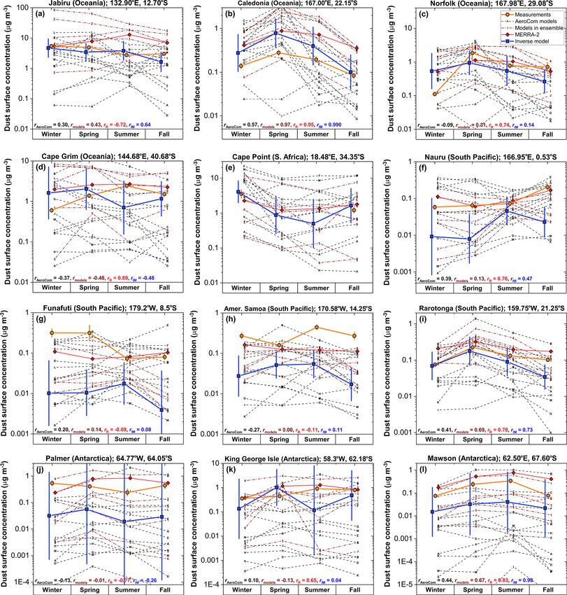
8130                                                              J. F. Kok et al.: Improved representation of the global dust cycle

Figure 1. Schematic of the methodology used to obtain an improved representation of the global dust cycle. Yellow boxes denote inputs
from an ensemble of global model simulations, blue boxes denote inputs from observational constraints on dust properties and abundance,
and white boxes denote the inverse model. We report the resulting representation of the global dust cycle in the present paper (green boxes)
and the partitioning of the global dust cycle by source region (magenta boxes) in our companion paper (Kok et al., 2021a). The subscripts
r, s, and k respectively refer to the originating source region, the season, and a model’s particle size bin. Other variables are defined in the
main text and the Glossary.

ties from Australia, southern Africa, and North and South                 the nine source regions. Specifically, we use simulations
America. Correspondingly, we divided the world into nine                  from the Community Earth System Model (CESM; Hur-
source regions that together account for the overwhelming                 rell et al., 2013; Scanza et al., 2018), IMPACT (Ito et al.,
majority (>99 %) of desert dust emissions simulated in mod-               2020), ModelE2.1 (Miller et al., 2006; Kelley et al., 2020),
els (Fig. 2a). Our analysis includes both natural and anthro-             GEOS/GOCART (Rienecker et al., 2008; Colarco et al.,
pogenic (land-use) emissions of dust in those source regions              2010), MONARCH (Pérez et al., 2011; Badia et al., 2017;
because our analysis is based on observations that by nature              Klose et al., 2021), and INCA/IPSL-CM6 (Boucher et al.,
integrate both (but see further discussion in Sect. 5.1). How-            2020). These six models were forced with three different re-
ever, our analysis explicitly does not include high-latitude              analysis meteorology datasets (Table 1), which helped sam-
dust sources, which produce dust through different mech-                  ple the uncertainty due to the exact reanalysis meteorology
anisms and with different properties than desert dust, yet                used that past work indicates is substantial (Largeron et al.,
likely dominate the dust loading for some high-latitude re-               2015; Smith et al., 2017; Evan, 2018). Most of the six models
gions (Prospero et al., 2012; Bullard et al., 2016; Tobo et               were run for the years 2004–2008 or a subset thereof to co-
al., 2019; Bachelder et al., 2020). The nine source regions               incide with the analysis period of regional DAOD in Ridley
partially follow the definition in Mahowald (2007), with the              et al. (2016), which provided most of observational DAOD
main difference that we divided the North African source re-              constraints used in this study (see Table 1). Sensitivity tests
gion, which accounts for approximately half of global dust                indicated that using different years from each simulation re-
emissions (Wu et al., 2020), into western North Africa, east-             sulted in differences of less than 10 % in the inverse model
ern North Africa, and the Sahel. Similar dust source regions              results. Each model either ran a separate simulation for each
were also used in more recent studies (Ginoux et al., 2012;               source region or used “tagged” dust tracers from each source
Di Biagio et al., 2017).                                                  region. The exact setup of each model is described in the
   We use an ensemble of global chemical transport and                    Supplement.
climate models (see Table 1) to obtain simulations of the                    Our inverse model uses several results derived from model
emission, transport, and deposition of dust from each of                  simulations (Fig. 1). First, for each model we obtained the

Atmos. Chem. Phys., 21, 8127–8167, 2021                                                       https://doi.org/10.5194/acp-21-8127-2021
J. F. Kok et al.: Improved representation of the global dust cycle                                                                       8131

Figure 2. Coordinates of (a) the nine main source regions and (b) the 15 observed regions with constraints on the regional dust aerosol optical
depth (DAOD), (c) dust surface concentration measurements, and (d) deposition flux measurements used in this study. The coordinates of
the nine source regions are as follows: (1) western North Africa (20◦ W–7.5◦ E; 18◦ N–37.5◦ N), (2) eastern North Africa (7.5–35◦ E; 18–
37.5◦ N), (3) the Sahel (20◦ W–35◦ E; 0–18◦ N), (4) the Middle East and central Asia (which includes the Horn of Africa; 35–75◦ E for
0–35◦ N, and 35–70◦ E for 35–50◦ N), (5) East Asia (70–120◦ E; 35–50◦ N), (6) North America (130–80◦ W; 20–45◦ N), (7) Australia
(110–160◦ E; 10–40◦ S), (8) South America (80–20◦ W; 0–60◦ S), and (9) southern Africa (0–40◦ E; 0–40◦ S). The coordinates and seasonal
DAOD of the 15 observed regions are listed in Table 2. Symbols in (c) and (d) denote groupings of observations by different regions. Made
with Natural Earth.

normalized seasonally averaged column loading l˜r,s,k (θ, φ),                We restricted our analysis to dust with a diameter D ≤
which is the spatial distribution of a unit (1 Tg) of loading             Dmax = 20 µm because there are insufficient measurements
originating from source region r for season s and particle                to constrain the abundance of coarser dust particles in
size bin k. As such, the units of this field are per square me-           the atmosphere (Adebiyi and Kok, 2020). Note, however,
ter (Tg m−2 loading per Tg of loading from source r), and we              that the few measurements that have been made of dust
show annual averages of the normalized bulk dust loading for              with D>20 µm suggest that it is abundant over and near
each model and source region in Fig. S1. Additionally, we                 source regions such as North Africa and accounts for a
obtained the normalized 3D concentration (C̃r,k,s (θ, φ, P );             non-negligible fraction of shortwave and longwave extinc-
m−3 ) and the 2D dust emission (F̃r,k,s (θ, φ); m−2 yr−1 ) and            tion (Ryder et al., 2019). As such, more measurements of
(dry and wet) deposition fluxes (D̃r,k,s (θ, φ); m−2 yr−1 ) that          “super-coarse” (D>10 µm) and “giant” (D>62.5 µm) dust
are associated with a unit of global dust loading for each                are needed, which would allow the analysis presented here
source region, season, and particle size bin. All model fields            to be extended to larger particle sizes in the future. Since
were regridded using a modified Akima cubic Hermite inter-                some of the models in our ensemble do not account for dust
polation (Akima, 1970) to a common resolution of 1.9◦ lat-                with D up to 20 µm, we use the procedure in Adebiyi et
itude by 2.5◦ longitude with 48 vertical levels (see Adebiyi              al. (2020; see their Sect. 2.3.1) to extend these models to
et al., 2020, for further details). As explained further below,           20 µm. Specifically, we use the normalized 12–20 µm particle
since our inverse model only uses normalized model fields                 size bin simulated by the GEOS/GOCART model to estimate
per particle size, our results are independent of model tuning            what CESM and GISS ModelE2.1 would have simulated for
of global dust emissions or the simulated relative contribu-              an additional particle size bin extending to 20 µm (see addi-
tions of the major source regions defined here (Fig. 1). Our              tional details in the Supplement). We chose this bin specifi-
results are also not affected by model errors in representing             cally from the GEOS/GOCART model because it shows the
dust mass extinction efficiency or the emitted dust size dis-             best agreement against the observational constraint on re-
tribution.                                                                gional DAOD (Fig. 3).

https://doi.org/10.5194/acp-21-8127-2021                                                    Atmos. Chem. Phys., 21, 8127–8167, 2021
8132                                                                              J. F. Kok et al.: Improved representation of the global dust cycle

Table 1. Overview of global model setups used in this study.

 Model        Model                  Spatial resolutionb                                                           Dust particle size bin      Simulation        Meteorological
 number       name                   (long × lat × level)                                                          diameter ranges (µm)           periodc        dataset used
 1            CESM/CAM4              2.5◦ × 1.9◦ × 56 levels                                    0.1–1; 1.0–2.5; 2.5–5; 5–10; 10–20a            2004–2008         ERA-Interim
 2            IMPACT                 2.5◦ × 2.0◦ × 59 levels                                        0.1–1.26; 1.26–2.5; 2.5–5; 5–20            2004–2005         MERRA2
 3            GISS ModelE2.1         2.5◦ × 2.0◦ × 40 levels             0.2–0.36; 0.36–0.6; 0.6–1.2; 1.2–2; 2–4; 4–8; 8–16; 16–20a            2004–2008         NCEP
 4            GEOS/GOCART            1.25◦ × 1.0◦ × 72 levels                                      0.2–2; 2–3.6; 3.6–6; 6–12; 12–20            2004–2008         MERRA2
 5            MONARCH                1.4◦ × 1.0◦ × 48 levels          0.2–0.36; 0.36–0.6; 0.6–1.2; 1.2–2; 2–3.6; 3.6–6; 6–12; 12–20            2004–2008         ERA-Interim
 6            INCA                   2.5◦ × 1.27◦ × 79 levels                                      0.2–2; 2–3.6; 3.6–6; 6–12; 12–20            2010–2014         ERA-Interim
a Denotes an additional bin added to the original model output in order to extend the particle diameter range to D
                                                                                                                   max = 20 µm. This additional bin was derived from the
GEOS/GOCART 12–20 µm particle size bin (see main text). b All model fields were regridded to a common resolution of 2.5◦ longitude by 1.9◦ latitude. c A multiyear
mean for each season was used.

2.2     Constraining the spatially resolved DAOD                                             particle size bin, in proportion to each bin’s contribution to
        corresponding to a unit (1 Tg) of bulk dust loading                                  the globally integrated loading produced by the source re-
                                                                                             gion, and then multiplying the size-resolved loading by the
We next implemented an inverse model to determine the opti-                                  mass extinction efficiency (MEE) to obtain the DAOD.
mal bulk dust loading that must be generated by each source                                      To obtain the Jacobian matrix in Eq. (1) we need to obtain
region to produce the best match against constraints on re-                                  f˘r,s,k , each particle bin’s fractional contribution to the glob-
gional DAOD. This inverse model thus requires the spatial                                    ally integrated dust loading generated by source region r in
pattern of DAOD produced per unit bulk dust loading from                                     season s. Because models as a group underestimate the mass
each source region, which is the Jacobian matrix of DAOD                                     of particles with larger diameters (D> ∼ 5 µm; Kok et al.,
with respect to dust loading. We obtained this DAOD pro-                                     2017), we adjust the model size distribution to match a con-
duced per unit (1 Tg) of bulk dust loading by combining the                                  straint on the globally averaged dust size distribution derived
simulated distributions of a unit of size-resolved dust loading                              from a combination of observations and models (Adebiyi and
(l˜r,s,k (θ φ)) with constraints on the globally averaged dust                               Kok, 2020). This procedure retains regional differences in the
size distribution and extinction efficiency (Kok et al., 2017;                               atmospheric dust size distribution that models simulated for
Adebiyi and Kok, 2020). The calculations of the Jacobian                                     the different source regions, while forcing the globally av-
matrix (this section) and the optimal bulk loading per source                                eraged dust size distribution that results from the summed
region (next section) are performed iteratively because each                                 contributions from all source regions to match the constraint
source region’s fractional contribution to global dust loading                               on the globally averaged dust size distribution. That is,
affects the agreement against the constraint on the globally
averaged dust size distribution.                                                                         αk f˜r,s,k
    The DAOD produced per unit of bulk dust loading origi-                                   f˘r,s,k = PN             ,                                                        (2)
                                                                                                          bins    ˜
                                                                                                        k=1 αk fr,s,k
nating from source region r in season s is (Kok et al., 2017)

                  ∂ τ̆r,s (θ, φ)       N
                                       Xbins                                                 where f˜r,s,k is the modeled mass fraction per particle size bin
Jr,s (θ, φ) =                      =            k f˘r,s,k l˜r,s,k (θ, φ)         (1)        for a given source region r and season s, and αk is the global
                      ∂ L̆r,s          k=1                                                   correction factor for particle size bin k, which is different for
where L̆r,s is the globally integrated bulk dust loading gen-                                each model. We obtained αk by setting the fraction of atmo-
erated by source region r in season s, τ̆r,s (θ, φ) is the spatial                           spheric dust in particle size bin k, summed over all source
distribution of DAOD due to dust from source region r in sea-                                regions and seasons, equal to the constraint on the fractional
son s, Jr,s is the Jacobian matrix (Tg−1 ) of τ̆r,s with respect                             contribution of particle size bin k to the global dust loading
to L̆r,s , Nbins is the number of particle size bins in a global                             from Adebiyi and Kok (2020). That is,
model simulation (or derived from the simulated modes),  k                                                           R Dk+ dV atm (D)
is the size-dependent mass extinction efficiency (m2 g−1 ) of                                                          Dk−        dD    dD
                                                                                             α k = PN P                                                          ,             (3)
particle size bin k defined further below, l˜r,s,k (θ, φ) (m−2 )
                                                                                                                                      . PN P
                                                                                                     sreg Ns             ˜                sreg Ns
                                                                                                         r         s=1 fr,s,k L̆r,s         r=1      s   L̆r,s
is the simulated seasonally averaged spatial distribution of
a unit of dust loading from source region r and particle bin                                 where Nsreg = 9 is the number of source regions (Fig. 2a)
k, and f˘r,s,k (unitless) is the fractional contribution of dust
loading in size bin k to the seasonally averaged      global dust                            and dV atm  (D)
                                                                                                               is a realization of the size-normalized (that
                                                                                                R DmaxdDdV atm
loading generated by source region r (i.e., k f˘r,s,k = 1). As
                                              P
                                                                                             is, 0        dD dD = 1, where Dmax = 20 µm) globally aver-
such, Eq. (1) obtains the DAOD produced per unit of dust                                     aged volume size distribution from Adebiyi and Kok (2020),
loading from a given source region and season by adding up                                   which was obtained by combining dozens of in situ measure-
the normalized spatial distributions of the loading from each                                ments of dust size distributions with an ensemble of climate

Atmos. Chem. Phys., 21, 8127–8167, 2021                                                                              https://doi.org/10.5194/acp-21-8127-2021
J. F. Kok et al.: Improved representation of the global dust cycle                                                            8133

model simulations. Further, Dk− and Dk+ are respectively the          We use joint observational–modeling constraints on re-
lower and upper diameter limits of particle size bin k, and        gional DAOD at 550 nm from Ridley et al. (2016). This study
L̆r,s is the globally integrated and seasonally averaged bulk      used three different satellite AOD retrievals – from the Multi-
dust loading per source region (as obtained from the analy-        angle Imaging Radiometer (MISR) and the Moderate Res-
sis below). As such, the denominator in Eq. (3) denotes the        olution Imaging Spectroradiometer (MODIS) on board the
simulated globally averaged mass fraction, whereas the nu-         Terra and Aqua satellites – and bias-corrected those satel-
merator denotes the globally averaged mass fraction in parti-      lite data using more accurate ground-based aerosol optical
cle size bin k as constrained from in situ measurements and        depth measurements from AERONET. Ridley et al. (2016)
model simulations by Adebiyi and Kok (2020).                       then used an ensemble of global model simulations to ob-
   The final ingredient needed to use Eq. (1) to obtain the        tain the fraction of AOD that is due to dust in 15 regions for
DAOD produced by a unit (1 Tg) of bulk dust loading from           which AOD is dominated by dust. Ridley et al. (2016) thus
a given source region and season is the MEE ( k ). We do          leveraged the strengths of these different tools by combining
not use each model’s assumed MEE because these tend to             the accuracy of ground-based measurements with the global
be substantially biased compared to measurements (Adebiyi          coverage of satellite retrievals and the ability of models to
et al., 2020). This bias is largely due to a neglect or under-     distinguish between different aerosol species. Furthermore,
estimation of the asphericity of dust (Huang et al., 2020),        by averaging the resulting DAOD over large areas and long
which increases the surface-to-volume ratio and thereby en-        time periods (2004–2008 for each season), this study min-
hances the MEE by ∼ 40 % (Kok et al., 2017). We thus fol-          imized representation errors that can affect model compar-
low Kok et al. (2017) in obtaining the MEE from constraints        isons to data (Schutgens et al., 2017). An additional strength
on the dust size distribution and the extinction efficiency of     of the Ridley et al. (2016) analysis is that it transparently
randomly oriented (Ginoux, 2003; Bagheri and Bonadonna,            propagates a range of uncertainties that are both observation-
2016) aspherical dust. That is,                                    ally and modeling based and which we in turn propagate into
            R Dk+ Qext (D) dV atm (D)                              our own analysis (see Sect. 2.5). We also consider the Ridley
         3 Dk−        D         dD    dD                           et al. (2016) dataset more accurate than aerosol reanalysis
k =                                     ,                 (4)
       2ρ d     R D k+ dV atm (D)
                                  dD                               products that assimilate similar AOD observations. This is
                  Dk−     dD                                       because the Ridley et al. (2016) product includes a transpar-
where Qext (D) is a realization of the globally averaged size-     ent quantification of errors that we propagated into the repre-
resolved extinction efficiency from the analysis of Kok et         sentation of the global dust cycle here and because the parti-
al. (2017), which is defined as the extinction cross sec-          tioning of assimilated AOD into different aerosol species in
tion divided by the projected area of a sphere with diame-         reanalysis products depends on the underlying aerosol mod-
ter D (π D 2 /4). The term dV atm (D)
                                        inside the integrals ap-   els and is thus susceptible to the large biases in the prognostic
                                dD                                 aerosol schemes of these models (e.g., Adebiyi et al., 2020;
proximates the sub-bin distribution in particle size bin k as
the globally averaged dust volume size distribution. Further,      Gliß et al., 2021). Nonetheless, the Ridley et al. (2016) data
ρ d = (2.5 ± 0.2) × 103 kg m−3 is the globally averaged den-       are subject to some important limitations discussed further in
sity of dust aerosols (Fratini et al., 2007; Reid et al., 2008;    Sect. 5.1.
Kaaden et al., 2009; Sow et al., 2009). This observation-             Although we consider the Ridley et al. (2016) constraints
ally constrained density of dust is lower than the 2600 to         on DAOD to be more accurate than constraints from individ-
2650 kg m−3 used in many models (Tegen et al., 2002; Gi-           ual satellite products, AERONET data, or aerosol reanalysis
noux et al., 2004), most likely because dust aerosols are ag-      products, this study’s results for the Southern Hemisphere
gregates with void space that lowers their density below that      (SH) are susceptible to substantial biases. This is because
of individual mineral particles.                                   dust makes up a substantially lower fraction of total AOD in
                                                                   the SH than for the main Northern Hemisphere (NH) source
2.3   Constraining the bulk dust loading generated by              regions (e.g., Fig. S2 in Kok et al., 2014a). Therefore, we did
      each source region                                           not use the Ridley et al. (2016) results for the SH and instead
                                                                   used the seasonally averaged DAOD estimated by Adebiyi
The above procedure combined model simulations of the 2D           et al. (2020) over the three SH regions. These DAOD con-
spatial variability of size-resolved dust loading with con-        straints are based on an ensemble of four aerosol reanalysis
straints on dust size distribution and MEE. This procedure         products, namely the Modern-Era Retrospective analysis for
yielded the spatial distribution of DAOD that is produced by       Research and Applications version 2 (MERRA-2; Gelaro et
a unit (1 Tg) of dust loading from a given source region and       al., 2017), the Navy Aerosol Analysis and Prediction Sys-
season. Next, we use an inverse modeling approach to deter-        tem (NAAPS; Lynch et al., 2016), the Japanese Reanalysis
mine how many teragrams (Tg) of loading are needed from            for Aerosol (JRAero; Yumimoto et al., 2017), and the Coper-
each source region to produce optimal agreement against            nicus Atmosphere Monitoring Service (CAMS) interim Re-
constraints on the seasonal DAOD over areas proximal to            analysis (CAMSiRA; Flemming et al., 2017). The resulting
major dust source regions.                                         regional DAOD product also includes an error estimation

https://doi.org/10.5194/acp-21-8127-2021                                            Atmos. Chem. Phys., 21, 8127–8167, 2021
8134 J. F. Kok et al.: Improved representation of the global dust cycle
based partially on the spread in DAOD in the four reanalysis L̆r,s that minimize the cost function of the summed squared
products. In addition, we added a region over North Amer- deviation (χτ2 ) between the 15 DAOD constraints and the cor-
ica, for which Ridley et al. (2016) did not obtain results and responding regional DAOD calculated from Eq. (7). That is
for which we also use the reanalysis-based results of Adebiyi (e.g., Cakmur et al., 2006),
et al. (2020). In total, we thus have constraints with error es-
p 2
XNτ,reg XNsreg p
timates on the seasonal and area-averaged DAOD over 15 χτ2 = p=1 r=1
L̆ r,s Jr,s − τ s , (8)
regions (see Fig. 2b and Table 2).
We then used an inverse modeling approach to deter- where Nτ,reg = 15 and Nsreg = 9. Because the variables in
mine the optimal combination of dust loadings from the nine Eqs. (1)–(8) are interdependent, we iterated these equations
source regions (denoted with subscript r) that minimizes the until convergence was achieved.
disagreement against the DAOD constraint of these 15 ob-
served regions (denoted with subscript p) for each season. 2.4 Obtaining constraints on DAOD, emission, loading,
We thus need to account for the contribution of each of the deposition, and concentration
nine source regions (Fig. 2a) to the DAOD in each of these
After constraining the seasonal dust loading L̆r,s generated
15 observed regions. The seasonally averaged DAOD over
by each source region, we now obtain the 2D DAOD and the
the observed region p is
size-resolved dust loading, emission and deposition fluxes,
p
XNsreg p and 3D concentration. We do so by using the fact that other
τs = Jr,s L̆r,s , (5)
r=1 dust cycle components (DAOD, concentration, deposition)
p scale linearly with dust loading because our model simula-
where τ s is the DAOD averaged over observed region p and
p p tions are driven by reanalysis products (Table 1) such that
season s, and Jr,s (Tg−1 ) is the Jacobian matrix of τ̆r,s with
p dust does not impact the meteorology. Each dust field can
respect to L̆r,s , where τ̆r,s denotes the area-averaged and sea-
therefore be obtained by multiplying the simulated normal-
sonally averaged DAOD over observed region p that is pro-
ized dust field (e.g., seasonal dust concentration per unit of
duced by dust from source region r. The Jacobian matrix
p dust loading) by the number of units of dust loading per
Jr,s is the area-weighted DAOD over observed region p that
source region and season (L̆r,s ).
is produced per unit of bulk dust loading originating from
p The 2D DAOD is then
source region r in season s. We obtain Jr,s by integrating XNsreg
Eq. (1) over Ap , the area of the observed region p (Table 2): τ̆s (θ, φ) = L̆ J (θ, φ) . (9)
r=1 r,s r,s
PNbins The size-resolved and bulk dust loadings are respectively
k f˘r,k l˜r,s,k (θ, φ) dA
R
p
p ∂ τ̆r,s Ap k=1
Jr,s = = R . (6) XNsreg
∂ L̆r,s Ap dA l˘s,k (θ, φ) = f˘ L̆ l˜ (θ, φ) , and (10)
r=1 r,k r,s r,s,k
XNbins XNsreg
The seasonally averaged globally integrated dust loading l˘s (θ, φ) = k=1
f˘ L̆ l˜
r=1 r,k r,s r,s,k
(θ, φ) . (11)
generated by each source region (L̆r,s ) is thus determined
from the number of units of dust loading from each source Similarly, the 3D size-resolved and bulk concentrations
region r that results in the best agreement against the con- produced by each source region are
p
straint on DAOD (τ s ) over the 15 observed regions. Equa- XNsreg
tion (5) thus represents a system of equations for each simu- C̆s,k (θ, φ, P ) = f˘ L̆ C̃
r=1 r,k r,s r,s,k
(θ, φ, P ) , and (12)
lation in our global model ensemble, which we can write in XNbins XNsreg
C̆s (θ, φ, P ) = k=1 r
f˘r,k L̆r,s C̃r,s,k (θ, φ, P ) , (13)
explicit matrix form for clarity:
h i where P is the vertical pressure level. And the size-resolved
N
τ 1s τ 2s · · · τ s τ,reg and bulk emission fluxes are
XNsreg
f˘ L̆ F̃
= L̆1,s L̆2,s · · · L̆Nsreg ,s F̆s,k (θ, φ) = r=1 r,k r,s r,s,k
(θ, φ) , and (14)
N
XNbins XNsreg
J1,s1 J1,s2 · · · J1,sτ,reg F̆s (θ, φ) = f˘r,k L̆r,s F̃r,s,k (θ, φ) . (15)
N k=1 r
· · · J2,sτ,reg
J1 J2,s2
2,s Finally, the size-resolved and bulk deposition fluxes are
. (7)
.. .. .. ..
. . . . XNsreg
f˘ L̆ D̃
Nτ,reg D̆s,k (θ, φ) = (θ, φ) , and (16)
JN1 sreg ,s JN2 sreg ,s · · · JNsreg ,s r=1 r,k r,s r,s,k
XNbins XNsreg
D̆s (θ, φ) = k=1
f˘ L̆ D̃
r=1 r,k r,s r,s,k
(θ, φ) . (17)
We used Eq. (7) to obtain the seasonally averaged global
dust loading generated by each source region. Specifically, See the Glossary for further descriptions of each variable.
for each season s we used the simplex search optimization In our companion paper (Kok et al., 2021a), we further par-
method (Lagarias et al., 1998) to determine the nine values of tition these fields into the originating source region.
Atmos. Chem. Phys., 21, 8127–8167, 2021 https://doi.org/10.5194/acp-21-8127-2021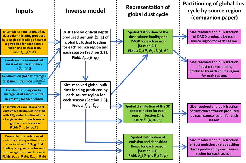
J. F. Kok et al.: Improved representation of the global dust cycle 8135
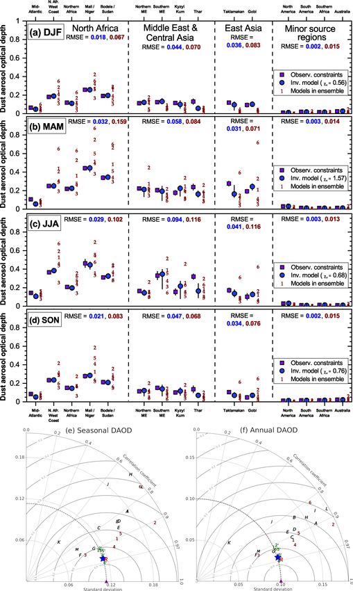
Table 2. Constraints on seasonal dust aerosol optical depth (DAOD) at 550 nm averaged over 15 regions. Regional DAOD constraints for
regions 1–11 are from Ridley et al. (2016) and were obtained using data from AERONET, MODIS, MISR, and a model ensemble. Regional
DAOD constraints for regions 12–15 are from Adebiyi et al. (2020) and were obtained from an ensemble of aerosol reanalysis products. All
constraints use data for the years 2004–2008.
Region Region Region DJF MAM JJA SON
number p name coordinates
1 Mid-Atlantic 20–50◦ W; 0.064 ± 0.013 0.106 ± 0.008 0.143 ± 0.005 0.084 ± 0.006
4–40◦ N
2 African west coast 20–5◦ W; 0.180 ± 0.010 0.250 ± 0.019 0.365 ± 0.016 0.233 ± 0.022
10–34◦ N
3 Northern Africa 5◦ W – 30◦ E; 0.118 ± 0.011 0.219 ± 0.010 0.207 ± 0.016 0.151 ± 0.016
26 – 40◦ N
4 Mali/Niger 5◦ W–10◦ E; 0.257 ± 0.019 0.441 ± 0.022 0.462 ± 0.044 0.277 ± 0.023
10–26◦ N
5 Bodele/Sudan 10–40◦ E; 0.191 ± 0.006 0.339 ± 0.023 0.310 ± 0.018 0.212 ± 0.021
10–26◦ N
6 Northern Middle East 30–50◦ E; 0.112 ± 0.011 0.223 ± 0.011 0.164 ± 0.015 0.113 ± 0.019
26–40◦ N
7 Southern Middle East 40–67.5◦ E; 0.123 ± 0.018 0.204 ± 0.021 0.330 ± 0.044 0.150 ± 0.020
0–26◦ N
8 Kyzyl Kum 50–67.5◦ E; 0.115 ± 0.017 0.176 ± 0.026 0.154 ± 0.034 0.101 ± 0.018
26–50◦ N
9 Thar 67.5–75◦ E; 0.130 ± 0.029 0.238 ± 0.033 0.319 ± 0.029 0.135 ± 0.037
20–50◦ N
10 Taklamakan 75–92.5◦ E; 0.119 ± 0.013 0.275 ± 0.027 0.171 ± 0.026 0.104 ± 0.011
30–50◦ N
11 Gobi 92.5–115◦ E; 0.093 ± 0.022 0.192 ± 0.022 0.102 ± 0.035 0.047 ± 0.021
36–50◦ N
12 North America 80–130◦ W; 0.010 ± 0.005 0.029 ± 0.011 0.028 ± 0.010 0.012 ± 0.006
20–45◦ N
13 South America 80–55◦ W; 0.019 ± 0.011 0.013 ± 0.007 0.010 ± 0.006 0.016 ± 0.009
0–55◦ S
14 Southern Africa 10–40◦ E; 0.016 ± 0.007 0.011 ± 0.005 0.013 ± 0.005 0.016 ± 0.007
10–35◦ S
15 Australia 110–160◦ E; 0.025 ± 0.013 0.013 ± 0.006 0.010 ± 0.005 0.023 ± 0.011
10–40◦ S
2.5 Improved model and inverse model results with First, we obtained improved model results by sampling
uncertainty over different realizations of observational constraints on
dust properties and abundance but using the output of only
The results represented by Eqs. (9)–(17) require realizations a single model. That is, we solved Eqs. (1)–(17) a large num-
of the various inputs (Fig. 1), which include both model fields ber of times (100; limited by computational resources), and
and constraints on dust properties and abundance. Because for each iteration we drew a random realization of each of the
each of these inputs is uncertain and as such is represented by observational constraints but used simulation results from a
a probability distribution, we obtained two products that sam- single model. This procedure thus includes a random draw-
ple different aspects of this uncertainty of the inputs, namely ing of realizations of the globally averaged dust size distribu-
“improved model” results and “inverse model” results. tion ( dV atm (D)
), the extinction efficiency (Qext (D)), the par-
dD
https://doi.org/10.5194/acp-21-8127-2021 Atmos. Chem. Phys., 21, 8127–8167, 2021
8136                                                        J. F. Kok et al.: Improved representation of the global dust cycle

                                                        p
ticle density (ρ d ), and the observed regional DAOD (τ s ). As       The bootstrap procedure used in the inverse model product
such, the improved model results represent output from a sin-      propagates all the quantified random and systematic errors
gle model (see Table 1) for which DAOD is calculated from          present in the inputs. Nonetheless, it cannot account for sys-
loading using the observational constraint on extinction effi-     tematic biases in these inputs, such as the tendency of models
ciency (Eq. 4) and for which the contributions from different      to underestimate coarse dust lifetime (Ansmann et al., 2017;
source regions and particle bins are added in such a way to        van der Does et al., 2018; Adebiyi et al., 2020). As such, the
simultaneously match observational constraints on the dust         obtained uncertainty ranges should be interpreted as a lower
size distribution (Eq. 2) and DAOD (Eq. 8).                        bound on the actual uncertainty.
   Second, we obtained our main product, namely the inverse
model product that represents the optimal representation of
the global dust cycle. We obtained this product by similarly       3     Comparison of inverse model results against
sampling over different realizations of the input fields, but            independent measurements and model simulations
now including a random drawing of one of the six global
model simulations in each of the bootstrap iterations. This        We evaluate the results of the inverse model described in
additional step propagates uncertainty in model predictions        the previous section using independent measurements of dust
of the normalized size-resolved dust loading, concentration,       surface concentration and deposition fluxes (Sect. 3.1). We
and deposition fields into our results (Eqs. 9–17). Because        also compare the inverse model results against the ensemble
different models use different particle size bins (Table 1), we    of AeroCom Phase I global dust cycle simulations (Huneeus
convert the size-resolved results from each bootstrap itera-       et al., 2011) and the MERRA-2 dust product (Sect. 3.2).
tion to common particles size bins of 0.2–0.5, 0.5–1, 1–2.5,
2.5–5, 5–10, and 10–20 µm. We do so by assuming that sub-          3.1    Independent dust measurements used to evaluate
bin distributions follow the constraint on the globally aver-             the inverse model
aged dust loading (Fig. 1). This assumption will introduce
some further error in size-resolved results. For both the in-      We use two sets of independent measurements to evaluate the
verse model and improved model products, we retained only          ability of the inverse model to reproduce the global dust cy-
those bootstrap iterations that produced a root mean square        cle. The first dataset is a compilation of dust surface concen-
error of less than 0.05 relative to the DAOD constraints; this     tration measurements. Of the 27 total stations in this compila-
quality control retained approximately three-quarters of the       tion, 22 are measurements of the bulk dust surface concentra-
iterations.                                                        tion taken in the North Atlantic from the Atmosphere–Ocean
   In drawing the realizations of seasonally averaged ob-          Chemistry Experiment (AEROCE; Arimoto et al., 1995) and
                     p
served DAOD (τ s ), we need to account for correlations of         taken in the Pacific Ocean from the sea–air exchange pro-
errors between different seasons and regions. Specifically,        gram (SEAREX; Prospero et al., 1989) for observation pe-
some of the errors in the calculation of the DAOD in Ridley        riods noted in Table 2 of Wu et al. (2020). These data were
et al. (2016) and Adebiyi et al. (2020) are systematic, such as    obtained by drawing large volumes of air through a filter. To
errors in satellite retrieval algorithms and systematic model      reduce the effects of anthropogenic aerosols, measurements
errors in simulations of (dust and non-dust) aerosols. These       were only taken when the wind was onshore and in excess
errors are thus at least partially correlated between seasons      of 1 m s−1 (Prospero et al., 1989). The mineral dust frac-
and regions, although we cannot establish the exact degree of      tion of the collected particulates was determined either by
correlation. We can thus roughly divide the errors into three      burning the sample and assuming the ash residue to repre-
different categories: errors that are completely random be-        sent the mineral dust fraction or from their Al content (as-
tween seasons and regions, systematic errors that are corre-       sumed to be 8 % for mineral dust, corresponding to the Al
lated between different seasons for the same region, and sys-      abundance in Earth’s crust) (Prospero, 1999). Note that since
tematic errors that are correlated across regions for a given      these measurements were taken during the period 1981–
season. The sum of the squared contributions of these three        2000, the dust surface concentration “climatology” obtained
                                              p
errors equals the square of the total error σ s reported in Ta-    from these measurements is for a different time period than
ble 2. Since we cannot determine what the relative contri-         that of the model simulations used in the inverse model (Ta-
bution of each of these three types of errors is, we assume        ble 1).
that the contribution of each of these three errors is equal.         Since most of the AEROCE and SEAREX stations are
Although the uncertainty in our results as quantified from         located far downwind of source regions, we also added a
the bootstrap procedure increases if a larger fraction of the      dataset of dust surface concentration from the Sahelian Dust
DAOD error is assumed to be systematic, the median results         Transect that was deployed in 2006 as part of the African
presented in Sect. 4 are not sensitive to the partitioning of      Monsoon Multidisciplinary Analysis (AMMA; Lebel et al.,
this error. The details of the mathematical treatment for cal-     2010; Marticorena et al., 2010). This dataset contains mea-
culating these errors are provided in the Supplement.              surements over 5–10 years of the surface concentration of
                                                                   aerosols with an aerodynamic diameter ≤ 10 µm (PM10,aer )

Atmos. Chem. Phys., 21, 8127–8167, 2021                                             https://doi.org/10.5194/acp-21-8127-2021
J. F. Kok et al.: Improved representation of the global dust cycle 8137
at four stations in the western Sahel (M’Bour, Bambey, Cin- 10 µm (PM10 ) from Albani et al. (2014). This study merged
zana, and Banizoumbou; see http://www.lisa.u-pec.fr/SDT/, data from previous datasets (Ginoux et al., 2001; Tegen et
last access: 13 May 2020). As with the AEROCE and al., 2002; Lawrence and Neff, 2009; Mahowald et al., 2009)
SEAREX datasets, only measurements were used for which and adjusted these data to cover the 0.1–10 µm geometric di-
the wind direction was predominantly coming from dust- ameter range. We obtained the PM10 deposition flux for the
dominated regions. As such, these measurements have at inverse model, the MERRA-2 data, and for each model in our
least two systematic errors: (i) the AMMA data reported the ensemble following the approach above for the PM10,aer con-
concentration of all particulate matter, so taking these mea- centration data. Note that we cannot correct the concentration
surements as being of dust concentration overestimates the and deposition flux of the AeroCom Phase I models (next
true dust concentration, and (ii) measurements taken when section) to the PM10,aer and PM10 size ranges because of a
wind was not coming from a dust-dominated region were lack of size-resolved simulation data. We thus used the bulk
omitted, which could also cause an overestimation of the dust concentration and deposition fluxes as many of these models
concentration. To mitigate the effect of this second error, we simulated the PM10 size range (see Table 3 in Huneeus et al.,
only use seasonally averaged dust concentrations for which 2011).
>70 % of data was retained. This resulted in the omission of To assess the consistency of the inverse model results
the winter and spring seasons at the Bambey station. with both the independent datasets, we calculated the error-
Following Huneeus et al. (2011) and Wu et al. (2020), we weighted mean square difference between the inverse model
additionally added surface concentration measurements of results and the observations. This statistic is known as the re-
PM10,aer dust from a long-term (May 1995–December 1996) duced chi-squared statistic and equals (Bevington and Robin-
filter-based deployment in Jabiru, northern Australia (Van- son, 2003)
derzalm et al., 2003). However, unlike Huneeus et al. (2011)
Ni
and Wu et al. (2020), we do not use data obtained in X (Mi − Oi )2
χν2 = , (19)
Rokumechi (Zimbabwe), which used a similar methodology, σi2 + σm2
i
because most of the dust at this southern African site orig-
inated locally from within and near the national park where where the index i sums over the Ni measurements in the
the station was located (p. 2649 in Nyanganyura et al., 2007). dataset, Oi is the ith measurement in the dataset, Mi is the
To use the measurements of PM10,aer dust in Jabiru and the inverse model result for the location and season of the ith
Sahel, we obtained the PM10,aer dust concentration for those measurement (if applicable), σm is the calculated error in
models with size-resolved surface concentrations, namely the inverse model result from the bootstrap procedure (see
the inverse model and each model in our ensemble. We Sect. 2.5), and σi is the error in the measurement. For a model
did so by first obtaining the geometric diameter that cor- that matches measurements within the experimental error,
responds to an aerodynamic diameter of 10 µm, which is χν2 ≈ 1 (Bevington and Robinson, 2003). Values of χν2 that
DPM10,aer = caer × 10 µm = 6.8 µm. This uses the conversion are
1 indicate an overestimate of model or experimental
factor caer = 0.68 from Huang et al. (2021), who accounted error, whereas values of χν2
1 indicate either an underes-
for the effects of particle shape (Huang et al., 2020) and den- timate of errors or substantial biases in the model or experi-
sity to link the aerodynamic and geometric diameters. For mental data.
each model, we then summed the contributions from par- We estimated the experimental errors in the surface con-
ticle bins with diameters smaller than DPM10,aer and used a centration measurements by propagating the standard error
correction factor cPM10,aer for particle size bins that straddle in monthly averaged surface concentration measurements
DPM10,aer . This correction factor uses the result from Adebiyi into seasonal and annual averages. Note that these errors do
and Kok (2020) that the globally averaged dust size distri- not include representation errors, which could be important
bution ( dVdlnD
atm (D)
) is approximately constant in the range of (Schutgens et al., 2017). The errors in deposition data are
5–20 µm such that the fractional contribution to the PM10,aer more difficult to estimate, as these are not usually reported
concentration of a bin that straddles DPM10,aer can be approx- and because deposition fluxes can show large spatial and
imated as temporal variability (Avila et al., 1997), leading to larger rep-
resentation errors. We estimated the relative error in deposi-
ln DPM10,aer /Dk− tion data measurements from the spread in measurements at
cPM10,aer = , (18)
ln Dk+ /Dk− similar locations. For the cluster of data in southern Europe
(eastern Spain, southern France, northern Italy; e.g., Avila et
where Dk− and Dk+ are respectively the lower and upper lim- al., 1997; Bonnet and Guieu, 2006), the standard deviation is
its of the particle size bin that straddles the 10 µm aerody- about an order of magnitude, and for clusters of data north
namic diameter (D = 6.8 µm). of Cape Verde (e.g., Jickells et al., 1996; Bory and Newton,
The second independent dataset that we used to evalu- 2000) and northwest of Tenerife (e.g., Honjo and Manganini,
ate the inverse model results is a compilation (110 stations) 1993; Kuss and Kremling, 1999), the standard deviation is
of the deposition flux of dust with a geometric diameter ≤ about a quarter of an order of magnitude. We therefore take
https://doi.org/10.5194/acp-21-8127-2021 Atmos. Chem. Phys., 21, 8127–8167, 2021You can also read