The penultimate deglaciation: protocol for Paleoclimate Modelling Intercomparison Project (PMIP) phase 4 transient numerical simulations between ...
←
→
Page content transcription
If your browser does not render page correctly, please read the page content below
Geosci. Model Dev., 12, 3649–3685, 2019
https://doi.org/10.5194/gmd-12-3649-2019
© Author(s) 2019. This work is distributed under
the Creative Commons Attribution 4.0 License.

The penultimate deglaciation: protocol for Paleoclimate Modelling
Intercomparison Project (PMIP) phase 4 transient numerical
simulations between 140 and 127 ka, version 1.0
Laurie Menviel1,* , Emilie Capron2,3,* , Aline Govin4 , Andrea Dutton5 , Lev Tarasov6 , Ayako Abe-Ouchi7 ,
Russell N. Drysdale8,9 , Philip L. Gibbard10 , Lauren Gregoire11 , Feng He12 , Ruza F. Ivanovic11 , Masa Kageyama4 ,
Kenji Kawamura13,14,15 , Amaelle Landais4 , Bette L. Otto-Bliesner16 , Ikumi Oyabu13 , Polychronis C. Tzedakis17 ,
Eric Wolff18 , and Xu Zhang19,20
1 Climate  Change Research Center, PANGEA, the University of New South Wales, Sydney, Australia
2 Physics  of Ice, Climate and Earth, Niels Bohr Institute, University of Copenhagen, Tagensvej 8, 2100 Copenhagen, Denmark
3 British Antarctic Survey, High Cross, Madingley Road, Cambridge, CB3 0ET, UK
4 Laboratoire des Sciences du Climat et de l’Environnement (LSCE), Institut Pierre Simon Laplace (IPSL),

CEA-CNRS-UVSQ, Université Paris-Saclay, Gif-Sur-Yvette, 91190, France
5 Department of Geological Sciences, University of Florida, P.O. Box 112120, Gainesville, FL 32611, USA
6 Department of Physics and Physical Oceanography, Memorial University of Newfoundland, St John’s, Canada
7 Atmosphere and Ocean Research Institute, The University of Tokyo, Tokyo, Japan
8 School of Geography, The University of Melbourne, Melbourne, Australia
9 Laboratoire EDYTEM UMR CNRS 5204, Université Savoie Mont Blanc, 73376 Le Bourget du Lac, France
10 Scott Polar Research Institute, University of Cambridge, Cambridge, CB2 1ER, UK
11 School of Earth and Environment, University of Leeds, Leeds, LS2 9JT, UK
12 Center for Climatic Research, Nelson Institute for Environmental Studies, University of Wisconsin-Madison,

Madison, WI 53706, USA
13 National Institute of Polar Research, Research Organizations of Information and Systems, 10-3 Midori-cho,

Tachikawa, Tokyo 190-8518, Japan
14 Department of Polar Science, Graduate University for Advanced Studies (SOKENDAI), 10-3 Midori-cho,

Tachikawa, Tokyo 190-8518, Japan
15 Institute of Biogeosciences, Japan Agency for Marine-Earth Science and Technology, 2-15 Natsushima-cho,

Yokosuka 237-0061, Japan
16 Climate and Global Dynamics Laboratory, National Center for Atmospheric Research (NCAR), Boulder, CO 80305, USA
17 Environmental Change Research Centre, Department of Geography, University College London, London, UK
18 Department of Earth Sciences, University of Cambridge, Cambridge, CB2 3EQ, UK
19 Alfred Wegener Institute, Helmholtz Centre for Polar and Marine Research, 27570 Bremerhaven, Germany
20 Key Laboratory of Western China’s Environmental Systems (Ministry of Education),

College of Earth and Environmental Sciences, Lanzhou University, Lanzhou, 730000, China
∗ These authors contributed equally to this work.

Correspondence: Laurie Menviel (l.menviel@unsw.edu.au) and Emilie Capron (capron@nbi.ku.dk)

Received: 11 February 2019 – Discussion started: 6 March 2019
Revised: 26 June 2019 – Accepted: 1 July 2019 – Published: 22 August 2019

Published by Copernicus Publications on behalf of the European Geosciences Union.
3650                                                                              L. Menviel et al.: Penultimate deglaciation

Abstract. The penultimate deglaciation (PDG, ∼ 138–128            Grant et al., 2014; Rohling et al., 2017). These long glacial
thousand years before present, hereafter ka) is the transition    periods were followed by relatively rapid multi-millennial-
from the penultimate glacial maximum (PGM) to the Last            scale warmings into consecutive interglacial states. These
Interglacial (LIG, ∼ 129–116 ka). The LIG stands out as one       deglaciations represent the largest natural global warming
of the warmest interglacials of the last 800 000 years (here-     and large-scale climate reorganizations across the Quater-
after kyr), with high-latitude temperature warmer than today      nary. Deglaciations are paced by an external forcing, i.e. vari-
and global sea level likely higher by at least 6 m. Considering   ations in the seasonal and latitudinal distribution of incoming
the transient nature of the Earth system, the LIG climate and     solar radiation (insolation) driven by changes in Earth’s orbit
ice-sheet evolution were certainly influenced by the changes      (Berger, 1978). However, changes in insolation alone are not
occurring during the penultimate deglaciation. It is thus im-     sufficient to explain the amplitude of these major warmings
portant to investigate, with coupled atmosphere–ocean gen-        and require amplification mechanisms. These amplification
eral circulation models (AOGCMs), the climate and envi-           mechanisms are related to the large increase in atmospheric
ronmental response to the large changes in boundary condi-        GHG concentrations (e.g. atmospheric CO2 increases by 60
tions (i.e. orbital configuration, atmospheric greenhouse gas     to 100 ppm; Lüthi et al., 2008), the disintegration of NH
concentrations, ice-sheet geometry and associated meltwater       ice sheets and their associated change in albedo (Abe-Ouchi
fluxes) occurring during the penultimate deglaciation.            et al., 2013), as well as changes in sea-ice and vegetation
   A deglaciation working group has recently been set up as       cover (Fig. 1). Hence, deglaciations provide a great oppor-
part of the Paleoclimate Modelling Intercomparison Project        tunity to study the interaction between the different compo-
(PMIP) phase 4, with a protocol to perform transient simula-      nents of the Earth System and climate’s sensitivity to changes
tions of the last deglaciation (19–11 ka; although the proto-     in radiative forcing.
col covers 26–0 ka). Similar to the last deglaciation, the dis-      A pervasive characteristic of the five deglaciations of the
integration of continental ice sheets during the penultimate      past 450 kyr is the occurrence of millennial-scale climate
deglaciation led to significant changes in the oceanic circu-     events (e.g. Cheng et al., 2009; Barker et al., 2011; Vázquez
lation during Heinrich Stadial 11 (∼ 136–129 ka). However,        Riveiros et al., 2013; Past Interglacials Working Group of
the two deglaciations bear significant differences in magni-      PAGES, 2016; Rodrigues et al., 2017). In the North Atlantic,
tude and temporal evolution of climate and environmental          these events, also referred to as stadials, are characterized
changes.                                                          by a substantial weakening of North Atlantic Deep Water
   Here, as part of the Past Global Changes (PAGES)-PMIP          (NADW) formation (e.g. McManus et al., 2004; Vázquez
working group on Quaternary interglacials (QUIGS), we pro-        Riveiros et al., 2013; Böhm et al., 2015; Ng et al., 2018),
pose a protocol to perform transient simulations of the penul-    possibly due to meltwater discharge into the North Atlantic
timate deglaciation under the auspices of PMIP4. This design      (Ivanovic et al., 2018). There is a link between these events
includes time-varying changes in orbital forcing, greenhouse      and enhanced iceberg calving, supported by the concurrent
gas concentrations, continental ice sheets as well as fresh-      presence of ice-rafted debris (IRD) in North Atlantic marine
water input from the disintegration of continental ice sheets.    sediment cores, and the stadials that contain substantial IRD
This experiment is designed for AOGCMs to assess the cou-         layers (identified as Heinrich events) are known as Heinrich
pled response of the climate system to all forcings. Addi-        stadials (e.g. Heinrich, 1988; Bond et al., 1992; McManus
tional sensitivity experiments are proposed to evaluate the       et al., 1999; van Kreveld et al., 2000; Hodell et al., 2017).
response to each forcing. Finally, a selection of paleo-records      A weakening of the Atlantic meridional heat transport dur-
representing different parts of the climate system is pre-        ing these stadials maintains cold conditions at high north-
sented, providing an appropriate benchmark for upcoming           ern latitudes in the Atlantic sector (Stouffer et al., 2007;
model–data comparisons across the penultimate deglacia-           Swingedouw et al., 2009; Kageyama et al., 2010, 2013)
tion.                                                             while contributing to a gradual warming at high southern
                                                                  latitudes (Blunier and Brook, 2001; Stocker and Johnsen,
                                                                  2003; EPICA community members, 2006), thus leading to
                                                                  a bipolar seesaw pattern of climate changes. The strengthen-
1   Introduction                                                  ing of NADW formation at the end of stadials induces a rel-
                                                                  atively abrupt temperature increase in the northern North At-
Over the last 450 kyr, Earth’s climate has been dominated         lantic and surrounding regions and a sharp increase in atmo-
by glacial–interglacial cycles with a recurrence period of        spheric CH4 and Asian monsoon strength (Loulergue et al.,
about 100 kyr. These asymmetrical cycles are characterized        2008; Cheng et al., 2009; Buizert et al., 2014). While a sig-
by long glacial periods, associated with a gradual cooling,       nificant atmospheric CO2 increase is also observed during
a slow decrease in atmospheric greenhouse gas (GHG) con-          the NADW recovery at the end of Heinrich stadials during
centrations and a progressive growth of large continental ice     deglaciations (Marcott et al., 2014), the major phase of at-
sheets in the Northern Hemisphere (NH), leading to a 60 to        mospheric CO2 increase coincides with a Southern Ocean
120 m global sea-level decrease (Lisiecki and Raymo, 2005;        (e.g. Barker et al., 2009; Uemura et al., 2018) and Antarctic

Geosci. Model Dev., 12, 3649–3685, 2019                                             www.geosci-model-dev.net/12/3649/2019/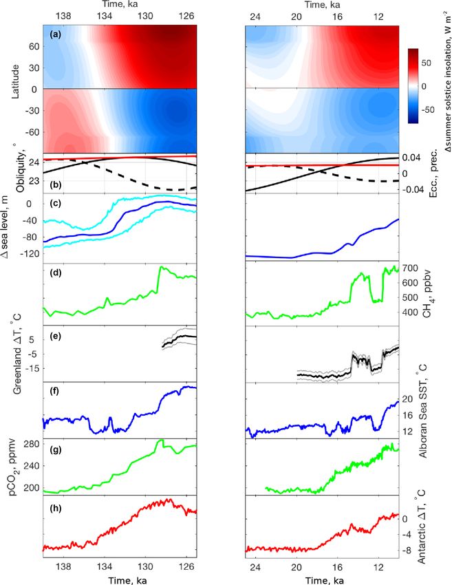
L. Menviel et al.: Penultimate deglaciation                                                                                               3651

Figure 1. Overview of (left) the penultimate and (right) the last deglaciations climatic and environmental evolutions: (a) Hovmöller diagram
of summer solstice insolation anomalies (W m−2 ). This corresponds to 21 June in the Northern Hemisphere and 21 December in the Southern
Hemisphere. Time series of (b) eccentricity (red), obliquity (solid black) and precession (dashed black) (Berger, 1978). (c) Global mean sea-
level anomaly probability maximum (m, blue), (left) including its 95 % confidence interval (cyan) (Grant et al., 2014), from Grant et al. (2012)
for the original age model for the penultimate and (right) from Lambeck et al. (2014) for the last deglaciation. (d) Atmospheric methane
(CH4 ) concentration as recorded in the EDC ice core, Antarctica (Loulergue et al., 2008). (e) Precipitation-weighted surface temperature
reconstruction based on stable water isotopes from the Greenland NEEM ice core (left) and annual surface temperature composite recon-
struction based on air nitrogen isotopes from the Greenland NEEM, NGRIP and GISP2 ice cores (Buizert et al., 2014). (f) Alkenone-based
(Uk’37 ) SST reconstruction from ODP976 (Martrat et al., 2014). (g) Atmospheric CO2 concentration as recorded in Antarctic ice cores for
(left) EDC (Bereiter et al., 2015) and (right) WAIS divide(Marcott et al., 2014) on the WD2014 chronology (Buizert et al., 2015). (h) Antarc-
tic temperature anomalies relative to the present day inferred from the EDC ice core (Jouzel et al., 2007). Unless specified differently, all
records are displayed on the AICC2012 timescale (Bazin et al., 2013; Veres et al., 2013) or a chronology coherent with AICC2012.

www.geosci-model-dev.net/12/3649/2019/                                                         Geosci. Model Dev., 12, 3649–3685, 2019
3652                                                                               L. Menviel et al.: Penultimate deglaciation

warming (Cheng et al., 2009; Masson-Delmotte et al., 2011;         et al., 2008), led to a warm period in the North Atlantic re-
Landais et al., 2013; Marcott et al., 2014) (Fig. 1). The se-      gion, the Bølling–Allerød (Liu et al., 2009; Buizert et al.,
quence of events leading to the deglacial atmospheric CO2          2014) (Fig. 1, right). This period of North Atlantic warm-
increase is still poorly constrained. Still, it most likely re-    ing coincides with (and may have triggered part of) the pe-
sulted from a combination of processes (e.g. Kohfeld and           riod of fastest sea-level rise, Meltwater Pulse-1A (MWP-1A)
Ridgwell, 2009), including changes in solubility, global al-       (Gregoire et al., 2016), during which sea level rose by 14–
kalinity content (e.g. Sigman et al., 2010), iron fertilization    18 m in less than 500 years, starting at ∼ 14.5 ka (e.g. De-
(e.g. Martin, 1990; Bopp et al., 2003; Martínez-García et al.,     schamps et al., 2012; Lambeck et al., 2014). At high southern
2014), Antarctic sea-ice cover (Stephens and Keeling, 2000)        latitudes, the gradual deglacial warming was interrupted by
and ocean circulation (e.g. Toggweiler et al., 2006; Ander-        the Antarctic Cold Reversal (ACR, ∼ 14.5–12.8 ka) (Jouzel
son et al., 2009; Skinner et al., 2010; Toggweiler and Lea,        et al., 1995, 2007; Pedro et al., 2016), which was also coinci-
2010). Changes in ocean circulation, and particularly varia-       dent with a pause in the deglacial atmospheric CO2 increase
tions in the formation rates of the main deep and bottom wa-       (e.g. Marcott et al., 2014). The ACR could be the result of
ter masses, i.e. NADW and Antarctic Bottom Water, can sig-         enhanced northward heat transport from the Southern Hemi-
nificantly impact atmospheric CO2 by modifying the vertical        sphere due to the strong NADW resumption occurring during
gradient in oceanic dissolved inorganic carbon (e.g. Menviel       the Bølling–Allerød (Pedro et al., 2016) or from a meltwater
et al., 2014, 2017, 2018).                                         pulse originating from the Antarctic ice sheet at the time of
   While they share similarities, the last two deglaciations       MWP-1A (Weaver et al., 2003; Menviel et al., 2011; Weber
also bear significant differences in amplitude and durations.      et al., 2014; Golledge et al., 2014).
Figure 1 shows the evolution of key variables across 15 kyr,          A return to stadial conditions over Greenland, Europe
from glacial maxima to peak interglacial conditions. The           and the North Atlantic occurred during the Younger Dryas
two deglaciations initiate under a range of glacial ice-sheet      (∼ 12.8–11.7 ka; Fig. 1, right) (Alley, 2000). This event
states and progress under a variety of orbital-forcing scenar-     likely resulted from a combination of processes (Renssen
ios (Tzedakis et al., 2017; Past Interglacials Working Group       et al., 2015), possibly including a weakening of NADW for-
of PAGES, 2016) (Fig. 1). Although there are still many            mation resulting from an increase in meltwater discharge into
open questions, the sequence of events occurring during the        the Arctic Ocean (Tarasov and Peltier, 2005; Murton et al.,
last deglaciation, which represents the transition from the        2010; Keigwin et al., 2018) or melting of the Fennoscan-
Last Glacial Maximum (LGM; Marine Isotope Stage 2, here-           dian ice sheet (Muschitiello et al., 2015), and an altered at-
after MIS2, 26–19 ka) to our current interglacial, is start-       mospheric circulation due to a minimum in solar activity
ing to emerge (Cheng et al., 2009; Denton et al., 2010;            (Renssen et al., 2000). While the Barbados coral record sug-
Shakun et al., 2012). The last deglaciation began with Hein-       gests that a second phase of rapid sea-level rise occurred at
rich Stadial 1 (HS1, ∼ 18–14.7 ka) when part of the Lau-           about 11.3 ka (MWP-1B) (e.g. Bard et al., 1990), data from
rentide and Eurasian ice sheets disintegrated (Dyke, 2004;         Tahiti boreholes (Bard et al., 2010) and from a compilation
Hughes et al., 2016), draining freshwater to the North At-         of sea-level data (Lambeck et al., 2014) provide no evidence
lantic, that may have contributed to the observed weakening        of a particularly rapid sea-level rise during that period.
of NADW formation (e.g. McManus et al., 2004; Gherardi                The penultimate deglaciation (∼ 138–128 ka, referred to
et al., 2009; Thornalley et al., 2011; Ng et al., 2018; Ivanovic   here as PDG), which represents the transition between
et al., 2018). HS1 was characterized by cold and dry con-          the penultimate glacial maximum (PGM) (MIS 6, also re-
ditions in the North Atlantic, over Greenland and Europe           ferred to as Late Saalian, 160–140 ka) and the Last Inter-
(Tzedakis et al., 2013; Buizert et al., 2014; Martrat et al.,      glacial (LIG; also referred to as MIS 5e in marine sediment
2014). Antarctic temperature and global atmospheric CO2            cores) (Govin et al., 2015), has received less attention. The
concentration rose during this period. Paleo-proxy records         PGM was characterized by an atmospheric CO2 content of
and modelling studies suggest that the Intertropical Conver-       ∼ 195 ppm (Lüthi et al., 2008) and a significantly differ-
gence Zone (ITCZ) shifted southward (e.g. Arz et al., 1998;        ent extent of NH ice sheets compared to the LGM (Dyke
Chiang and Bitz, 2005; Timmermann et al., 2005; Stouffer           et al., 2002; Svendsen et al., 2004; Lambeck et al., 2006;
et al., 2007; Kageyama et al., 2009, 2013; Marzin et al., 2013;    Ehlers et al., 2011; Margari et al., 2014). The eustatic sea
McGee et al., 2014), thus leading to dry conditions in most        level during the PGM is estimated at ∼ 90–100 m lower than
of the northern tropics, including the northern part of South      present-day values (Rabineau et al., 2006; Grant et al., 2012;
America (Peterson et al., 2000; Deplazes et al., 2013; Mon-        Rohling et al., 2017), with a relatively large uncertainty range
tade et al., 2015) and the Sahel (Mulitza et al., 2008; Nie-       (Rohling et al., 2017). This compares to ∼ 130 m lower or
dermeyer et al., 2009). Chinese speleothem records also in-        more than during the present day during the LGM (Auster-
dicate a weak East Asian summer monsoon activity during            mann et al., 2013; Lambeck et al., 2014). The LIG also bears
HS1 (Wang et al., 2001; Cheng et al., 2009).                       significant differences to the interstadial that followed the
   The abrupt NADW resumption at ∼ 14.7 ka, imprinted by           last deglaciation, i.e. the Holocene. Latest data-based esti-
a sharp atmospheric CH4 concentration increase (Loulergue          mates suggest that sea level was ∼ 6 to 9 m higher during

Geosci. Model Dev., 12, 3649–3685, 2019                                              www.geosci-model-dev.net/12/3649/2019/
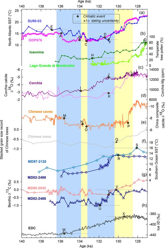
L. Menviel et al.: Penultimate deglaciation                                                                                  3653

the LIG than today, thus implying a significant ice-mass loss       due to the melting of NH ice sheets could explain the rela-
from both the Greenland and Antarctic ice sheets (e.g. Dutton       tively cold conditions in the North Atlantic and warm con-
et al., 2015). In addition, compared to pre-industrial times,       ditions in the Southern Ocean observed in paleo-data dur-
high-latitude sea surface temperature (SST) and Greenland           ing these time periods (Govin et al., 2012; Stone et al.,
surface temperatures were respectively ≥ 1 ◦ C and 3 to 11 ◦ C      2016). However, snapshot experiments assume that the cli-
greater during the LIG (e.g. Landais et al., 2016; Capron           mate state is in near-equilibrium, and because relatively rapid
et al., 2017; Hoffman et al., 2017). Considering the transient      and large changes in both internal and external forcings oc-
nature of the Earth system, a better understanding of the PDG       cur during deglaciations, transient simulations (i.e. numeri-
could thus improve our knowledge of the processes that led          cal simulations with time-varying boundary conditions) are
to continental ice-mass loss during the LIG.                        needed. These simulations also allow a more robust paleo-
   Recent work (Masson-Delmotte et al., 2011; Landais et al.,       data–modelling comparison, thus enabling the refinement of
2013; Govin et al., 2015) also depicted a sequence of events        the sequence of events.
over the PDG that contrasts with the one across the last               Transient numerical simulations have already been per-
deglaciation. Paleo-proxy records indicate that the disinte-        formed for the last deglaciation (Liu et al., 2009; Menviel
gration of NH ice sheets induced a ∼ 80 m sea-level rise            et al., 2011; Roche et al., 2011; Gregoire et al., 2012; He
(Grant et al., 2014) between 135 and 129 ka. This is also           et al., 2013; Otto-Bliesner et al., 2014) and provide a dynam-
concomitant with Heinrich Stadial 11 (HS11) (e.g. Hein-             ical framework to further our understanding of the climate-
rich, 1988; Oppo et al., 2006; Skinner and Shackleton, 2006;        change drivers, teleconnections and feedbacks inherent in the
Govin et al., 2015). HS11 was characterized by weak NADW            Earth system. Currently, no three-dimensional transient sim-
formation (Oppo et al., 2006; Böhm et al., 2015; Deaney             ulations were run across the full time interval covered by
et al., 2017), cold and dry conditions in the North Atlantic        the penultimate deglaciation (∼ 140–127 ka). However, tran-
region (Drysdale et al., 2009; Martrat et al., 2014; Marino         sient simulations covering the period 135 to 115 ka have been
et al., 2015), and gradually warmer conditions over Antarc-         performed with a range of models to understand the impact
tica (Jouzel et al., 2007), associated with a sustained atmo-       of surface boundary conditions and freshwater fluxes on the
spheric CO2 increase of ∼ 60 ppm between ∼ 134 and 129 ka           LIG (Bakker et al., 2013; Loutre et al., 2014; Goelzer et al.,
(Landais et al., 2013) (Figs. 1, 2). Increasing evidence of sub-    2016a). The need for transient simulations is now recog-
millennial-scale climate changes at high and low latitudes          nized, and a protocol to perform transient experiments of the
during HS11 (e.g. Martrat et al., 2014) prompts the need to         last deglaciation as part of Paleoclimate Modelling Intercom-
refine the sequence of events across the PDG. However, this         parison Project (PMIP) phase 4 has been recently established
is challenging as (i) climatic reconstructions over the PDG         (Ivanovic et al., 2016). However, to further our understand-
are still scarce and most records have insufficient resolution      ing of the processes at play during deglaciations, including
to allow the identification of centennial- to millennial-scale      the role of millennial-scale climate change, other deglacia-
climatic variability and (ii) it is difficult to establish robust   tions should be studied in detail. Transient simulations of the
absolute and relative chronologies for most paleo-climatic          penultimate deglaciation could also help to understand the
records across this time interval (Govin et al., 2015).             climate and sea-level highstand occurring during the LIG.
   While our knowledge of the processes and feedbacks oc-           We thus propose to extend the PMIP4 working group on
curring during deglaciations has significantly improved over        the last deglaciation to include the penultimate deglaciation
the last two decades (e.g. Cheng et al., 2009, 2016; Shakun         and thus create a deglaciation working group. This effort
et al., 2012; Abe-Ouchi et al., 2013; Landais et al., 2013),        will complement the last deglaciation experiments of PMIP4
many unknowns remain. For example, our understanding of             (Ivanovic et al., 2016), allowing an evaluation of the similar-
the precise roles of atmospheric and oceanic processes in           ities and differences in the climate system response during
leading to the waning of glacial continental ice sheets dur-        the last and the penultimate deglaciations.
ing deglaciations is still incomplete. It is also crucial to com-      Here we present a protocol to perform transient numeri-
prehend the subsequent impacts of continental ice-sheet dis-        cal simulations of the PDG from 140 to 127 ka with coupled
integration on the oceanic circulation, climate, the terrestrial    atmosphere–ocean general circulation models (AOGCMs).
vegetation and the carbon cycle system.                             These experiments will provide a link with the PMIP4 tran-
   Numerical simulations performed with climate models              sient LIG experiment (127 to 121 ka) (Otto-Bliesner et al.,
provide a dynamical framework to understand the response            2017). After a description of changes in insolation (Sect. 2),
of the Earth system to external forcing (i.e. insolation) and       GHGs (Sect. 3), continental ice sheets (Sect. 4) and sea level
internal dynamics (e.g. albedo, GHGs) that culminate in             (Sect. 5) occurring during the PDG, we present a frame-
deglaciations. Atmospheric and oceanic teleconnections as-          work to perform transient simulations of PDG (Sects. 6 and
sociated with millennial-scale variability can also be stud-        7), as well as a selection of key paleo-climate and paleo-
ied in detail. Model–paleo-climate proxy comparisons, in-           environmental records to be used for model–data compar-
cluding snapshot experiments at 130 and at 126 ka, suggest          isons (Sect. 8).
that the inclusion of freshwater forcing in the North Atlantic

www.geosci-model-dev.net/12/3649/2019/                                                Geosci. Model Dev., 12, 3649–3685, 2019
3654                                                                                 L. Menviel et al.: Penultimate deglaciation

                                                                      tion period, ranging from 0.033 at 140 ka to 0.041 at 127 ka,
                                                                      and is significantly higher than during the last deglaciation
                                                                      (Fig. 1b; ∼ 0.019 at the LGM to 0.020 at 14 ka) and than
                                                                      the present value of 0.0167. Obliquity peaks at 131 ka; the
                                                                      degree of tilt is similar between the last and the penultimate
                                                                      deglaciation. Perihelion occurs near the NH winter solstice
                                                                      at 140 ka, shifting to near the NH summer solstice by 127 ka.
                                                                         Although the overall trends in summer solstice insolation
                                                                      anomalies, as compared to the mean of the last 1000 years,
                                                                      evolve similarly in the last and penultimate deglaciations,
                                                                      the magnitudes of the maximum positive summer anomalies
                                                                      in the NH and the minimum negative summer anomalies in
                                                                      the Southern Hemisphere are much greater during the PDG,
                                                                      when eccentricity is higher, than during the last deglacia-
                                                                      tion (Fig. 1a). At 65◦ N, peak summer anomalies of more
                                                                      than 70 W m−2 occur at 128 ka. In contrast, during the last
                                                                      deglaciation, the 65◦ N summer solstice anomalies peak at
                                                                      11 ka, with anomalies of ∼ 50 W m−2 . Similarly, 65◦ S sum-
                                                                      mer solstice negative anomalies are close to −40 W m−2 at
                                                                      127 ka but only about −20 W m−2 at 10 ka. In addition, the
                                                                      rates of change in summer solstice anomalies are greater
                                                                      from 140 to 127 ka than from 21 to 8 ka.
                                                                         Given the clear differences between the solar forcing of
                                                                      last and penultimate deglaciations, comparing the two tran-
                                                                      sient deglacial simulations will provide valuable information
                                                                      on the underlying mechanisms and Earth system feedbacks.
Figure 2. Atmospheric greenhouse gas concentrations: atmospheric
trace gases through the penultimate deglaciation from Antarctic ice   The solar constant should be set to 1360.7 W m−2 , consis-
cores displayed on the AICC2012 chronology (Bazin et al., 2013;       tent with the Coupled Model Intercomparison Project phase
Veres et al., 2013) and the spline that should be used to force the   6 (CMIP6)–PMIP4 piControl and lig127k simulations (Otto-
transient simulations (solid and dotted black lines; Köhler et al.,   Bliesner et al., 2017) as well as the PMIP4 transient climate
2017a). (a) Atmospheric CO2 concentrations from EDC (turquoise        simulation of the last deglaciation (Ivanovic et al., 2016).
and blue) (Lourantou et al., 2010; Schneider et al., 2013) and
TALDICE (green) (Schneider et al., 2013). (b) Atmospheric CH4
concentration from EDC (Loulergue et al., 2008) (blue), Vostok (Pe-   3   Greenhouse gases
tit et al., 1999) (orange), TALDICE (Buiron et al., 2011) (green)
and EDML (Capron et al., 2010) (pink). (c) Atmospheric N2 O con-
                                                                      GHG records are available solely from Antarctic ice cores
centration from EDC (Flückiger et al., 2002) (blue), EDML (Schilt
                                                                      across the time interval 140–127 ka (Fig. 2). LIG GHG
et al., 2010) (pink) and TALDICE (Schilt et al., 2010) (green). Due
to in situ production within the ice sheet, no accurate N2 O mea-     records from North Greenland Eemian Ice Drilling (NEEM)
surements are available beyond 134.5 ka. Between 140 and 134.5 ka     and other Greenland ice cores are affected by stratigraphic
N2 O should increase linearly from 201 to 218.74 ppb (dashed black    disturbances and in situ CO2 , CH4 and N2 O production
line). Red crosses indicate the 140 ka spin-up values for CO2 , CH4   (e.g. Tschumi and Stauffer, 2000; NEEM community mem-
and N2 O concentrations (i.e. 191 ppm, 385 and 201 ppb, respec-       bers, 2013). The North Greenland Ice Project (NGRIP) ice
tively).                                                              core provides a continuous and reliable CH4 record, but it
                                                                      only extends back to ∼ 123 ka (North Greenland Ice Core
                                                                      project members, 2004). We first briefly describe existing
2   Insolation                                                        atmospheric CO2 , CH4 and N2 O records (below). The re-
                                                                      cent spline-smoothed GHG curves calculated from a selec-
The orbital parameters (eccentricity, obliquity and longitude         tion of those records (Köhler et al., 2017a) should be used.
of perihelion) should be time evolving and set following              They have the benefit of providing continuous GHG records,
Berger (1978). This external forcing affects the seasonal and         with a temporal resolution of 1 year on the commonly used
latitudinal distribution, as well as the magnitude of solar en-       AICC2012 gas-age scale (Bazin et al., 2013; Veres et al.,
ergy received at the top of the atmosphere and, in the case           2013). This timescale is associated with an average 1σ ab-
of obliquity (Earth’s axial tilt), the annual mean insolation at      solute error of ∼ 2 kyr between 140 and 127 ka.
any given latitude with opposite, but small, effects at low and          Atmospheric CO2 concentrations have been measured
high latitudes. Eccentricity is high during the entire deglacia-      on the EPICA Dome C (EDC) and Talos Dome Ice core

Geosci. Model Dev., 12, 3649–3685, 2019                                                www.geosci-model-dev.net/12/3649/2019/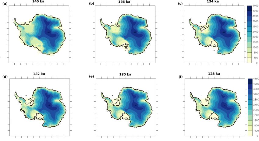
L. Menviel et al.: Penultimate deglaciation                                                                                  3655

(TALDICE) ice cores (Fig. 2). The EDC records from                terwards. No reliable atmospheric N2 O concentrations are
Lourantou et al. (2010) and Schneider et al. (2013) agree         available beyond 134 ka as N2 O concentrations measured
well overall. The Schneider et al. (2013) dataset depicts a       in the air trapped in ice from the PGM are affected by in
long-term CO2 increase starting at ∼ 137.8 ka and ending at       situ production related to microbial activity (Schilt et al.,
∼ 128.5 ka with a centennial-scale CO2 rise above the sub-        2010). During the LGM (considered here as the time inter-
sequent LIG CO2 values, also referred to as an “overshoot”.       val 26–21 ka), the average N2 O level was ∼ 201 ppb. As-
The CO2 overshoot is smaller in the Schneider et al. (2013)       suming the LGM is an analogue for the PGM, we propose
dataset compared to a similar feature measured in Lourantou       a 140 ka spin-up value and N2 O transient forcing curve that
et al. (2010): while the former displays a relatively constant    starts with a 201 ppb level and then linearly increases to
CO2 concentration of ∼ 275 ppm between 128 and 126 ka,            218.74 ppb at 134.5 ka. From 134.5 ka, the N2 O smoothed
the latter shows a CO2 decrease from 280 to 265 ppm be-           spline curve calculated by Köhler et al. (2017a), which is
tween 128 and 126 ka. The offsets between CO2 records             based on the TALDICE and EDC discrete N2 O measure-
from the same EDC core are likely related to the different        ments, should be used.
air extraction techniques used in the two studies (Schneider         The CO2 and N2 O levels from the spline curves at 127 ka
et al., 2013). The smoothed spline CO2 curve, which should        (274 ppm and 257 ppb) only differ from the values chosen
be used as forcing for the PDG is based on those two EDC          as boundary conditions for the PMIP4 lig127k equilibrium
datasets and the calculation method accounts for such poten-      experiment by 1 ppm and 2 ppb respectively (Otto-Bliesner
tial difference in local maxima (details provided in Köhler       et al., 2017; Köhler et al., 2017a). The comparison is less di-
et al., 2017a).                                                   rect for CH4 . Indeed, a global CH4 value (685 ppm) rather
   Atmospheric CH4 concentration records from Vostok,             than an Antarctic ice-core-based CH4 value (e.g. CH4 level
EPICA Dronning Maud Land (EDML), EDC and TALDICE                  of 660 ppm at 127 ka in Köhler et al., 2017a) is proposed
agree well within the gas-age uncertainties attached to each      as forcing for the lig127k simulations. However, this differ-
core (Fig. 2). They illustrate a slow rise from ∼ 390 to          ence in global atmospheric CH4 and Antarctic ice-core CH4
540 ppb between ∼ 137 and 129 ka, which is followed by an         concentration is similar to the one observed during the mid-
abrupt increase of ∼ 200 ppb reaching maximum LIG val-            Holocene (23 ppb) (Otto-Bliesner et al., 2017; Köhler et al.,
ues at ∼ 128.5 ka. Because CH4 sources are located mostly         2017a).
in the NH, an interpolar concentration difference (IPD) be-
tween Greenland and Antarctic CH4 records exists.
   For instance, an IPD of ∼ 14, ∼ 34 and ∼ 43 ppb is re-         4   Continental ice sheets
ported during the LGM, Heinrich Stadial 1 and the Bølling
                                                                  Changes in continental ice sheets during the deglaciation will
warming respectively (Baumgartner et al., 2012). However,
                                                                  significantly impact the climate system through their albedo,
without reliable CH4 records from Greenland ice cores, it re-
                                                                  which will directly affect the radiative balance (e.g. He et al.,
mains challenging to estimate the evolution of the IPD across
                                                                  2013). Changes in continental ice-sheet geometry can also
the deglaciation. Hence, for the atmospheric CH4 forcing of
                                                                  significantly impact atmospheric dynamics (e.g. Zhang et al.,
transient PDG simulations, the smoothed spline CH4 curve,
                                                                  2014; Gong et al., 2015). Transient simulations of the PDG
which is solely based on the EDC CH4 record (Köhler et al.,
                                                                  will thus need to be forced by the three-dimensional and
2017a) should be used, recognizing that the values may be
                                                                  time-varying evolution of continental ice sheets, which is
1 %–4 % lower than the actual global average.
                                                                  currently only available from numerical simulations. How-
   Both CO2 and CH4 concentrations undergo some rapid
                                                                  ever, simulating the evolution of continental ice sheets across
changes around 140 ka, which is also the time when the mod-
                                                                  the PDG is associated with large uncertainties, due to the cli-
els should spin up. To avoid possible artificial abrupt changes
                                                                  mate forcing of the ice-sheet models and poorly constrained
in the GHG, the average values obtained for the interval 139–
                                                                  non-linearities within the ice-sheet system. Glacial geologi-
141 (i.e. 191 ppm for CO2 and 385 ppb for CH4 , Table 1)
                                                                  cal data (e.g. glacial deposits and glacial striations) are also
should be used as spin-up CO2 and CH4 concentrations. Con-
                                                                  available to constrain continental ice-sheet evolutions and
sequently, CO2 and CH4 changes between 140 and 139 ka
                                                                  can thus provide an estimate of the uncertainties associated
provided in the forcing scenarios are linearly interpolated
                                                                  with the numerical ice-sheet evolutions. In this section, we
between the 140 ka spin-up values and those at 139 ka of
                                                                  describe the available numerical ice-sheet evolutions to use
196.68 ppm for CO2 and 287.65 ppb for CH4 . From 139 ka,
                                                                  as a forcing of the transient simulations of the PDG. We fur-
the spline-smoothed curves from Köhler et al. (2017a) should
                                                                  ther compare the results of these simulations with existing
be used.
                                                                  glacial geological constraints.
   Atmospheric TALDICE, EDML and EDC N2 O records
are available between 134.5 and 127 ka (Fig. 2) (Schilt et al.,
2010; Flückiger et al., 2002). From 134.5 to 128 ka, N2 O
levels increase from ∼ 220 to 270 ppb. Following a short
decrease until ∼ 127 ka, N2 O concentrations stabilize af-

www.geosci-model-dev.net/12/3649/2019/                                              Geosci. Model Dev., 12, 3649–3685, 2019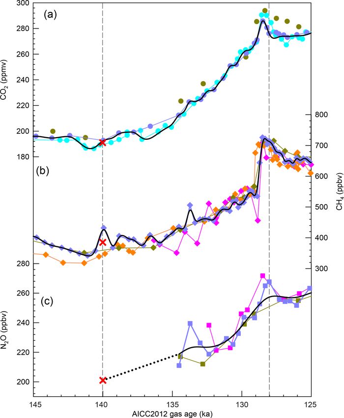
3656                                                                                     L. Menviel et al.: Penultimate deglaciation

Table 1. Summary of forcings and boundary conditions to apply for the PGM spin-up (140 ka) and subsequent transient simulation of the
PDG.

      Forcing                         140 ka spin-up       Transient simulation (140–127 ka)
                                      PDGv1-PGMspin        PDGv1
      Orbital parameters
      Eccentricity                    0.033                from Berger (1978)
      Obliquity                       23.414◦              from Berger (1978)
      Perihelion – 180◦               73◦                  from Berger (1978)
      Atmospheric greenhouse gases concentrations
      on the AICC2012 chronology (Bazin et al., 2013; Veres et al., 2013)
      CO2                             191 ppm              spline from Köhler et al. (2017a) based on the EDC records
                                                           (Lourantou et al., 2010; Schneider et al., 2013)
      CH4                             385 ppb              spline from Köhler et al. (2017a) based on the EDC record
                                                           (Loulergue et al., 2008)
      N2 O                            201 ppb              linear increase from 201 ppb at 140 ka to 218.74 ppb at 134.5 ka
                                                           spline from Köhler et al. (2017a) based on the EDC and TALDICE records
                                                           (Schilt et al., 2010; Spahni et al., 2005)
      Ice sheets
      North American and Eurasian     140 ka               IcIES-NH (Abe-Ouchi et al., 2013)
      Greenland                       140 ka GSM-G         GSM-G (Tarasov et al., 2012)
      Antarctica                      140 ka GSM-A         GSM-A (Briggs et al., 2014)
      Bathymetry and orography
      Bering Strait                   closed               gradual opening consistent with sea-level rise
      Sunda and Sahul shelves         emerged              gradual flooding consistent with sea-level rise
      Freshwater input
      Northern Hemisphere             none                 based on sea-level changes (fSL, blue in Fig. 4f)
      Antarctic coast                 none                 0.0135 Sv between 140 and 130 ka (constant rate)

4.1    Combined ice-sheet forcing                                       Nares Strait ranging to a few hundred metres in elevation dif-
                                                                        ference.
To facilitate the transient simulations of the PDG, we pro-                From the LIG onward, the combined ice-sheet evolution,
vide a combined ice-sheet forcing (available in the Supple-             referred to as GLAC-1D in PMIP4, is used (e.g. Ivanovic
ment and on the PMIP4 wiki), in which separate recon-                   et al., 2016). GLAC-1D includes the Greenland and Antarc-
structions of different ice sheets have been merged. As the             tic ice-sheet components described in Sect. 4.3 and 4.4
sea-level solver assumes an equilibrium initial condition, the          (Briggs et al., 2014), the North American ice-sheet simula-
simulations start at the previous interglacial. As is standard,         tion described in Tarasov et al. (2012), and the Eurasian ice-
the solver also requires present-day ice-sheet histories to             sheet simulation described in Tarasov (2014). The ice-sheet
bias-correct against present-day observed topography. Thus,             thickness from these simulations is run through a sea-level
a full 240 kyr ice-sheet history is required. The simulated             solver using the Viscosity Model (VM5a) (Peltier and Drum-
NH ice-sheet evolution, described in Sect. 4.2 (Abe-Ouchi               mond, 2008) Earth rheology to extract a gravitationally self-
et al., 2013), is merged with the simulated Greenland and               consistent topography. The surface topography is then run
the Antarctic (Briggs et al., 2014) evolutions described in             through a global surface drainage solver (using the algorithm
Sect. 4.3 and 4.4, respectively. The resolution of the merged           described in Tarasov and Peltier, 2006) to extract the rele-
ice-sheet file is 1◦ longitude by 0.5◦ latitude. The merger in-         vant surface drainage pointer field for each time slice. This
volves no extra smoothing, beyond that inherent in the glacial          will indicate into which ocean grid cell each terrestrial grid
isostatic adjustment solver, which involves transformation to           cell will drain.
spherical harmonics. The merger involves a simple masking
operation with the mask boundary through Nares Strait, Baf-
fin Bay, Davis Strait and the Labrador Sea. Examination of
the resultant topography shows small merger artefacts around

Geosci. Model Dev., 12, 3649–3685, 2019                                                    www.geosci-model-dev.net/12/3649/2019/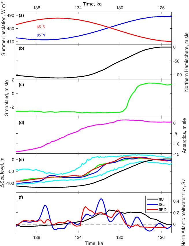
L. Menviel et al.: Penultimate deglaciation                                                                                   3657

4.2   North American and Eurasian ice sheets                        tion produces a ∼ 24 m sle contribution from Eurasia. Thus,
                                                                    the volume of the North American ice sheet may also be over-
The evolution of NH ice sheets during the PDG is given              estimated.
by a numerical simulation performed with the thermo-                   In the ice-sheet simulation, NH ice-mass loss closely fol-
mechanically coupled ice-sheet model IcIES (Ice-sheet               lows the boreal summer insolation and occurs mostly be-
model for Integrated Earth system Studies) with an original         tween ∼ 134 and 127 ka (Fig. 4), with two peaks of glacial
resolution of 1◦ by 1◦ in the horizontal and 26 vertical lev-       meltwater release at ∼ 131 and 128 ka. By 132 ka, the
els (Abe-Ouchi et al., 2007) (Fig. 3). IcIES uses the shallow       Eurasian ice sheet has decreased significantly and the south-
ice approximation and computes the evolution of grounded            ern and western flanks of the North American ice sheet have
ice but not floating ice shelves. The sliding velocity is re-       disintegrated (Fig. 3). Another significant retreat of the North
lated to the gravitational driving stress according to Payne        American ice sheet occurs between 132 and 128 ka, at which
(1999) and basal sliding only occurs when the basal ice is at       point it is mostly restricted to the north of the Hudson Bay.
the pressure melting point. This ice-sheet model was driven         By 127 ka, the North American ice sheet only remains over
by climatic changes obtained from the MIROC general cir-            Baffin Island.
culation model (GCM) (Abe-Ouchi et al., 2013), which was
forced by changes in insolation and atmospheric CO2 con-
                                                                    4.3   Greenland ice sheet
centration. In global agreement with glacial geological con-
straints (Dyke et al., 2002; Svendsen et al., 2004; Curry et al.,
2011; Syverson and Colgan, 2011) and other numerical sim-           The Greenland model uses an updated version
ulations of NH ice-sheet evolution (Tarasov et al., 2012; Abe-      (GSM.G7.31.18) of the Glacial Systems Model (e.g.
Ouchi et al., 2013; Peltier et al., 2015; Colleoni et al., 2016),   Tarasov et al., 2012) run at grid resolution of 0.5◦ longitude
the simulated extent and volume of the North American ice           by 0.25◦ latitude. The model has been upgraded to hybrid
sheet was smaller during the PGM than the LGM (Fig. 3).             shallow-ice and shallow-shelf physics, with an ice dynam-
   In Eurasia, the PGM recorded the most extensive glacia-          ical core from Pollard and DeConto (2012) and includes
tion since MIS 12 (Hughes and Gibbard, 2019). The max-              a 4 km deep permafrost-resolving bed thermal component
imum extent of the Fennoscandian ice sheet probably oc-             (Tarasov and Peltier, 2007), a viscoelastic bedrock response
curred at ∼ 160 ka, when it extended into the central Nether-       with global ice-sheet and sea-level loading, sub-shelf melt,
lands, Germany and the Russian Plain (Margari et al., 2010;         parametrizations for subgrid mass-balance and ice flow (Le
Ehlers et al., 2011; Hughes and Gibbard, 2019). This was            Morzadec et al., 2015), and updated parametrizations for
followed by a partial melting of the Fennoscandian ice sheet,       surface mass-balance and ice calving.
peaking between ∼ 157 and 154 ka, and a readvance after                Given that with active bed thermodynamics (down to
150 ka (Margari et al., 2010; Hughes and Gibbard, 2019).            4 km), the thermodynamic equilibration timescale is greater
The maximum extent of the NH ice sheets probably occurred           than 100 kyr for the Greenland ice sheet, the most appropriate
at the end of the PGM (Margari et al., 2014; Head and Gib-          method is to start the run during the previous interglacial pe-
bard, 2015). In Europe the late PGM ice advance was less            riod. Therefore, the model runs start at 240 ka with present-
expensive than at ∼ 160 ka but that was compensated for             day ice and bedrock geometry and with an ice and bed tem-
by ice-sheet expansion in Russia, Siberia (Astakhov et al.,         perature field from the end of a previous 240 ka model run.
2016) and North America (e.g. Curry et al., 2011; Syver-            The model is then forced from 240 ka until 0 ka, with a cli-
son and Colgan, 2011). Glacial geological constraints (e.g.         mate forcing that is partly glacial-index-based, using a com-
Astakhov, 2004; Svendsen et al., 2004) indeed suggest that          posite of a glaciological inversion of the GISP2 regional tem-
the Barents–Kara ice sheet extended further during the PGM          perature change (for the last 40 kyr) and the synthetic Green-
than the LGM. The simulated Eurasian ice sheet is in general        land δ 18 O curve that was deduced from the Antarctic EDC
agreement with the reconstruction of Lambeck et al. (2006),         isotopic record assuming a thermal bipolar seesaw pattern
with a dome reaching 3000 m over the Kara Sea during the            (Barker et al., 2011). The climate forcing also includes a two-
PGM that subsequently disintegrated across the deglaciation.        way coupled 2-D energy balance climate model (Tarasov and
However, the extent and volume of the simulated Eurasian            Peltier, 1997) to capture radiative changes.
ice sheet might be underestimated since it is smaller at the           Greenland ice-sheet model runs are scored against a large
PGM than LGM, whereas reconstructions suggest it should             set of constraints including relative sea-level (RSL), prox-
be larger at the PGM (Lambeck et al., 2006; Rohling et al.,         imity to present-day ice-surface topography, present-day ob-
2017).                                                              served basal temperatures from various ice cores, time of
   Rohling et al. (2017) further suggest that the ice volume        deglaciation of Nares Strait and the location of the present-
was almost equally distributed between Eurasia and North            day summit. The last 20 kyr of the run is critical as this rep-
America at the PGM, with a 33 to 53 m global mean sea-level         resents the time period with most of the data constraints for
equivalent (sle) contribution from the Eurasian ice sheet and       Greenland. The simulation presented here (G9175) is a least
39–59 m from North America, whereas the ice-sheet simula-           misfit model from a preliminary exploratory ensemble.

www.geosci-model-dev.net/12/3649/2019/                                                Geosci. Model Dev., 12, 3649–3685, 2019
3658 L. Menviel et al.: Penultimate deglaciation
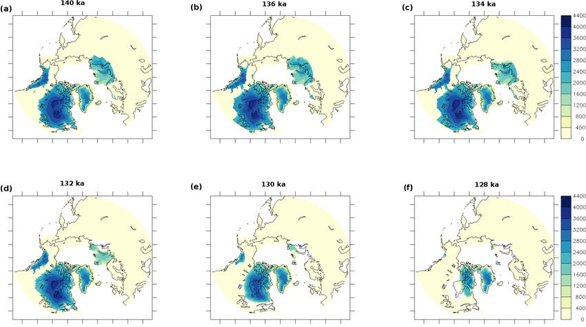
Figure 3. NH ice-sheet elevation (m) at (a) 140, (b) 136, (c) 134, (d) 132, (e) 130 and (f) 128 ka from the combined ice-sheet forcing as
simulated by the IcIES-MIROC model (Abe-Ouchi et al., 2013) for the North American and Eurasian ice sheets and as simulated by the
Glacial Systems Model (GSM) (e.g. Tarasov et al., 2012) for the Greenland ice sheet. Elevation is shown where the ice mask is greater
than 0.5.
This simulation suggests no significant change in Green- core drilled at that site (NEEM community members, 2013).
land ice mass until ∼ 134 ka (Fig. 4), followed by a small ice- Based on the paleo-proxy records and model simulations, the
mass loss, mostly from floating ice, between 134 and 130 ka. protocol for the PMIP4 LIG simulation for 127 ka (lig127k)
In this simulation, the main phase of Greenland deglacia- recommends a pre-industrial Greenland configuration.
tion occurs between 130 and 127 ka, during which Green-
land loses an ice mass of 2.9 m sle in excess of the total pre-
4.4 Antarctic ice sheet
industrial value and then an additional 1.5 m sle. As shown
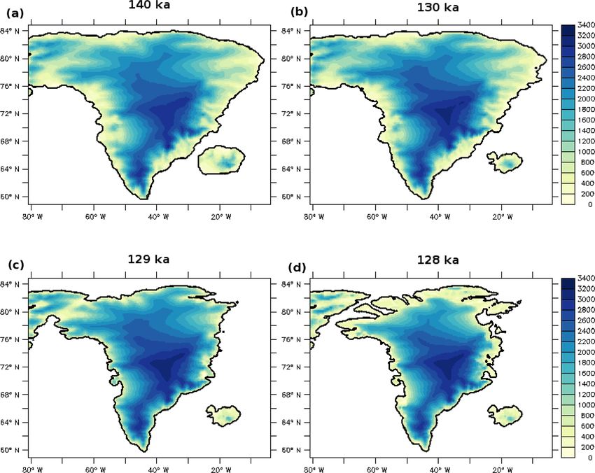
in Fig. 5, the extent and height of the Greenland ice sheet is
significantly smaller at 128 ka than at 132 ka. Greenland ice- The Antarctic model configuration is largely that of Briggs
mass loss is particularly evident on its western side, with a et al. (2013, 2014): a hybrid of the Penn State University ice-
part of southwestern Greenland being ice-free. To a first or- sheet model (Pollard and DeConto, 2012) and the GSM. Sim-
der, the simulated disintegration of the Greenland ice sheet ulations are run with a 40 km grid resolution using the LR04
follows the increase in boreal summer insolation and in at- benthic δ 18 O stack (Lisiecki and Raymo, 2005, referred to
mospheric CO2 (Fig. 1). as LR04) for sea-level forcing. The climate forcing is a para-
The main phase of the Greenland ice-sheet retreat in metric mix of an index-based approach (using the EDC δD
this simulation is globally in agreement with proxy records, record of Jouzel et al., 2007) and one based on orbital forc-
which suggest significant runoff in the Labrador Sea at ing, as detailed by Briggs et al. (2013). The parameter vector
∼ 130 ka and at ∼ 127 ka (e.g. Carlson and Winsor, 2012). (nn4041 from Briggs et al., 2014) that gave the best fit to
However the simulated Greenland ice-sheet disintegration constraints (GSM-A) in the large ensemble analysis is used.
could be too rapid as paleo-proxy records suggest significant Two changes are imposed on the model to partially rectify
meltwater discharge from the Greenland ice sheet through- an inadequate LIG sea-level contribution. First, SST depen-
out the LIG (e.g. Carlson and Winsor, 2012). In addition, dence is added to the sub-shelf melt model. Second, to com-
other model simulations suggest a maximum sea-level con- pensate for inadequate LIG warming, where SSTs are above
tribution from Greenland at ∼ 123–121 ka (Yau et al., 2016; present-day values, they are then given a minimum value of
Bradley et al., 2018), in agreement with the timing of the LIG 3 ◦ C (i.e. SST = MAX(SST, 3.0 ◦ C)). Even so, the Antarc-
minimum elevation at the Greenland NEEM location. This tic contribution to the LIG highstand is only 1.4 m sle and is
minimum elevation estimate was reconstructed from total air therefore inadequate given current inferences (as well as con-
content and water isotopic records measured on the deep ice straints on contributions from Greenland and steric effects)
(e.g. Kopp et al., 2009).
Geosci. Model Dev., 12, 3649–3685, 2019 www.geosci-model-dev.net/12/3649/2019/L. Menviel et al.: Penultimate deglaciation 3659
5 Sea level
Direct evidence for constraining the evolution of the global
sea level during the time interval 140–127 ka remains sparse.
Although the LR04 benthic δ 18 O stack (Lisiecki and Raymo,
2005) is sometimes used to approximate sea-level change on
glacial–interglacial timescales, in the case of the PDG, the
timing of the LR04 benthic δ 18 O stack is fixed by reference
to a handful of U-series coral dates from Huon Peninsula
with relatively high analytical uncertainties and questionable
preservation (Bard et al., 1990; Stein et al., 1993). Tying the
MIS 5e peak to the average age of these coral dates results in
a benthic δ 18 O minimum that is roughly centred on the main
phase of coral growth during this interglacial period (122–
129 ka) (Stirling et al., 1998) rather than having the onset of
the interglacial aligned with the timing of the onset of the
sea-level highstand at far-field sites (∼ 129 ka) (e.g. Stirling
et al., 1998; Dutton et al., 2015).
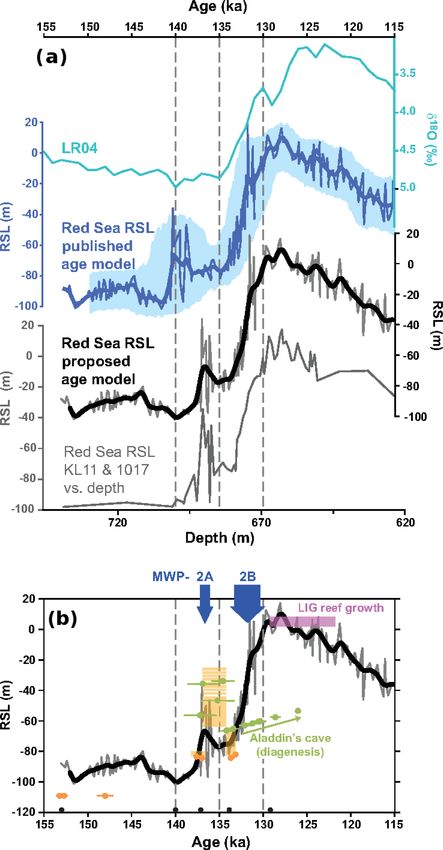
Here, we seek to provide an improved reconstruction
of sea level across the PDG by examining available RSL
records. Information on the timing and magnitude of the
changes across this time interval is provided by three RSL
records (Fig. 7):
(i) An RSL record from the Red Sea (Grant et al., 2012),
that is deduced from the planktic foraminifera δ 18 O
Figure 4. Time series of (a) summer solstice insolation at 65◦ N measured on sediment cores retrieved in this evapora-
and 65◦ S, (b)–(d) global sea-level equivalent (m) of changes in (b) tive marginal sea. This record is transformed into an
NH (Abe-Ouchi et al., 2013), (c) Greenland (Tarasov et al., 2012) RSL signal by using hydraulic models that constrain the
and (d) Antarctic ice sheets (Briggs et al., 2014), (e) and global salinity of surface waters as a function of sea level. The
sea-level (m) change estimated from Red Sea records (Grant et al., Red Sea record provides the only continuous profile of
2014) (green) with the 95 % probability interval (cyan), sea-level RSL across our interval of interest;
record with an adjusted age scale as described in Sect. 5 (blue) and
as estimated from the continental ice-sheet simulations (black). The (ii) RSL data from the U-series dates and elevations of the
red line shows the changes in global sea level that would be obtained submerged coral reefs of Tahiti (Thomas et al., 2009);
by adding the meltwater flux, fIRD, described in (f) plus an Antarc- and
tic contribution of 13 m. (f) Possible North Atlantic meltwater flux
(Sv) scenarios: estimated from the disintegration of NH ice sheets (iii) RSL data derived from U-series dates and elevations of
as shown in (b, c) (Tarasov et al., 2012; Abe-Ouchi et al., 2013) uplifted coral terraces of Huon Peninsula, Papua New
(black), estimated from the global sea-level change on the revised Guinea (Esat et al., 1999).
age scale (this study, blue) and scaled from the North Atlantic and
Norwegian Sea IRD records (red, shown in Fig. 8b). Providing a robust age model for sediment records from
the PGM to the LIG is not straightforward (e.g. Govin et al.,
2015), and over time, several age models have been proposed
for the Red Sea RSL record (e.g. Siddall et al., 2003; Rohling
et al., 2009; Grant et al., 2012). The latest chronology is
The simulation suggests a continuous Antarctic ice-sheet based on climatic alignment of the Red Sea RSL record to
discharge during the PDG, with a glacial ice-mass loss of eastern Mediterranean planktic foraminifera δ 18 O records,
∼ 12.5 m sle between 140 and 131 ka, followed by an addi- which are in turn aligned to the absolutely dated Soreq Cave
tional 1.4 m sle between 131 and 130 ka (Fig. 4). In this simu- speleothem δ 18 O record (Grant et al., 2012). While the ab-
lation, the West Antarctic ice sheet loses significant ice mass solute ages of the speleothem record have the potential to
between 140 and 136 ka (Fig. 6), with a retreat of the ground- provide a more robust age model (both in terms of accuracy
ing line over the Ross Sea as well as ice-mass loss in the and precision), the application of these dates to the Red Sea
Weddell Sea, on the Antarctic Peninsula and in the Amund- sea-level reconstruction hinges on the assumption that the
sen Sea sector. By 132 ka, the grounding line has completely tie points between the Red Sea and eastern Mediterranean
retreated over the Ross Sea and has retreated significantly records have been correctly assigned, and that the intervals
over the Weddell Sea. between these tie points can be linearly extrapolated.
www.geosci-model-dev.net/12/3649/2019/ Geosci. Model Dev., 12, 3649–3685, 20193660 L. Menviel et al.: Penultimate deglaciation Figure 5. Greenland ice-sheet elevation (m) at (a) 140 ka, (b) 130 ka, (c) 129 ka and (d) 128 ka as simulated by the GSM (e.g. Tarasov et al., 2012). The 0 elevation contour is in black. Figure 6. Antarctic ice-sheet elevation at (a) 140 ka, (b) 136 ka, (c) 134 ka, (d) 132 ka, (e) 130 ka and (f) 128 ka as simulated by the GSM (e.g. Briggs et al., 2014). Grounding lines are in black. Geosci. Model Dev., 12, 3649–3685, 2019 www.geosci-model-dev.net/12/3649/2019/
L. Menviel et al.: Penultimate deglaciation                                                                                   3661

   The Tahiti and Huon Peninsula corals are associated with        this diagenetic array of data from Aladdin’s Cave is a bet-
absolute radiometric dates (using U-series geochronology).         ter approximation for the primary age (i.e. it is closer to the
For the purpose of this study, all of the U-series ages have       unaltered endmember). Despite these diagenetic concerns,
been recalculated to normalize them with the same set of de-       the agreement in the timing of this PDG sea-level reversal
cay constants for 234 U and 230 Th (Cheng et al., 2013) (Ta-       (MWP-2A) in Tahiti and Huon Peninsula is striking (Fig. 7b).
bles S3 and S4), using the methodology described by Hibbert            When considering the 95 % probabilistic intervals of the
et al. (2016). The array of data from Huon Peninsula sug-          Red Sea RSL reconstruction on the chronology from Grant
gests post-depositional alteration (open-system behaviour of       et al. (2012), an overlap is observed with the coral data over
the U-series isotopes) that complicates a precise age interpre-    the MWP-2A interval, within the stated uncertainties. Still,
tation (Fig. 7).                                                   both coral datasets suggest that MWP-2A occurs several mil-
   The Red Sea time series published by Grant et al. (2012)        lennia later (i.e. ∼ 135–134 ka) than in the Red Sea RSL re-
shows that, after an RSL low stand of about −100 m relative        construction. This mismatch is likely to be related to the diffi-
to present between 145 and 141 ka, a brief pulse of at least       culty of precisely anchoring the dating of the current Red Sea
∼ 25 m sea-level rise, based on the smoothed record (or up         RSL age scale over this interval (as also discussed in the Sup-
to ∼ 50 m based on the unsmoothed time series), occurred           plement of Grant et al., 2012). Hence, we propose a revised
between ∼ 141 and 138 ka (identified as MWP-2A in Marino           chronology for the Red Sea RSL record in order to provide a
et al., 2015; Fig. 7a). This pulse was followed by a slight sea-   better agreement with the absolutely dated corals. Given the
level fall (∼ 10 m in the smoothed record) between ∼ 139           potential ambiguities of the tie point defined in Grant et al.
and 138 ka. Finally, a more significant pulse of ∼ 70 m in         (2012) to stretch the depth scale across this interval, we find
RSL rise (MWP-2B) is inferred between 135 and 130 ka. The          it reasonable to adjust it such that the timing of MWP-2A is
period between the ephemeral pulse of sea-level rise at the        more consistent with the absolute ages provided by the Tahiti
beginning of the PDG (MWP-2A) and the second prolonged             and Huon Peninsula coral data.
pulse (MWP-2B/HS11) has sometimes been referred to as                  We note that reassigning the tie points across this inter-
the PDG sea-level reversal (Siddall et al., 2006).                 val (Table S5), where tie points are placed at the beginning
   The coral RSL data from Huon Peninsula and Tahiti in-           and end of MWP-2A (as defined by the coral data), results
dependently provide additional evidence for an ephemeral           in a sea-level reconstruction that more closely approximates
reversal in sea-level rise occurring during the penultimate        a linear age–depth model (Fig. 7a). This revised age model
deglaciation (Fig. 7). In the case of Tahiti, sedimentary ev-      for the Red Sea RSL is adopted as our preferred reconstruc-
idence for the superposition of shallow and deeper water           tion for sea-level change during the PDG. This reconstruc-
facies led to the interpretation that there was an ephemeral       tion also compresses the total duration of the sea-level rise
deepening (sea-level rise) followed by a return to shallower       during the entirety of the PDG transition, which has impli-
water conditions (sea-level fall or stabilization) (Thomas         cations for the freshwater forcing in the NH and for making
et al., 2009). The Tahiti data provide bounding ages on the        analogies between the last and penultimate deglaciations.
timing of this sea-level rise pulse, with ages of corals that          This revised chronology is still attached to large uncertain-
grew at 135.0 ka (in 0–6 m water depth) and 133.5 (±1) ka          ties given the limits of the datasets. Also, considerable uncer-
(0–25 m water depth). In between these shallower facies,           tainties remain with the magnitude of the sea-level pulse dur-
there is a deeper water facies (≥ 20 m paleo-water depth),         ing MWP-2A because some of the corals cover a wide range
but there are no reliable ages within this interval of the core    of paleo-water depth (0 to 6 m for the pre-MWP-2A Tahiti
(Thomas et al., 2009). This observation, based on changes          corals, ≥ 20 m for the Tahiti corals during MWP-2A, 0–25 m
in both the lithofacies and benthic foraminiferal assemblage,      for the post-MWP-2A Tahiti corals and 0 to 20 m for the Al-
is interpreted as a pulse of sea-level rise in between about       addin’s Cave corals). Despite these uncertainties in the ab-
135.0 and 133.5 ka (Fujita et al., 2010). A similar sea-level      solute position of sea level, the relative sea-level changes for
oscillation has also been interpreted based on the stratigra-      each site clearly demonstrate an ephemeral deepening during
phy as well as the age and paleo-water depth reconstruction        meltwater pulse MWP-2A in both cases.
at Huon Peninsula (Esat et al., 1999). The absolute timing of          Glacial isostatic adjustment to the deterioration of the
coral growth is only loosely constrained at this site due to the   PGM ice sheets will also differentially affect Tahiti and Huon
open-system behaviour of the U-series isotopes (as reflected       Peninsula, which precludes a direct comparison of the mag-
by the scatter in ages of corals collected in Aladdin’s Cave,      nitude of sea-level change between these sites or a direct in-
∼ 134 to 126 ka; Fig. 7) (Esat et al., 1999). Indeed, the corals   terpretation of global mean sea-level change in the absence of
from Terrace VII have ages (with high uncertainty) ranging         modelling. Because the changes in global mean sea level are
from about 137 to 134.5 ka and the corals from the cave have       rapid across the penultimate deglaciation, the eustatic signal
a wide range of ages, from 134.1 to 125.9 ka (more details         is likely dominant, leading to a timing of the rapid changes
in Esat et al., 1999). Given that the younger end of this age      that is similar between local RSL and global mean sea-level
range is clearly within the MIS 5e sea-level highstand (e.g.       reconstructions. Still, the rate of change may be different
Stirling et al., 1998), it is more likely that the older end of    between sites due to local differences in the magnitude of

www.geosci-model-dev.net/12/3649/2019/                                               Geosci. Model Dev., 12, 3649–3685, 2019
You can also read