The MONASH Style of Computable General Equilibrium Modeling: A Framework for Practical Policy Analysis
←
→
Page content transcription
If your browser does not render page correctly, please read the page content below
CHAPTER       2
  The MONASH Style of Computable
  General Equilibrium Modeling: A
  Framework for Practical Policy Analysis
  Peter B. Dixon, Robert B. Koopman, Maureen T. Rimmer

  Centre of Policy Studies, Monash University

   US International Trade Commission

  Abstract
       MONASH models are descended from Johansen's 1960 model of Norway. The first MONASH model
       was ORANI, used in Australia's tariff debate of the 1970s. Johansen's influence combined with insti-
       tutional arrangements in their development gave MONASH models distinctive characteristics, facili-
       tating a broad range of policy-relevant applications. MONASH models currently operate in numerous
       countries to provide insights on a variety of questions including:
            the effects on:
                 macro, industry, regional, labor market, distributional and environmental variables
            of changes in:
                 taxes, public consumption, environmental policies, technologies, commodity prices, interest
                 rates, wage-setting arrangements, infrastructure and major-project expenditures, and known
                 levels and exploitability of mineral deposits (the Dutch disease).
       MONASH models are also used for explaining periods of history, estimating changes in technologies
       and preferences and generating baseline forecasts. Creation of MONASH models involved a series of
       enhancements to Johansen's model, including: (i) a computational procedure that eliminated
       Johansen's linearization errors without sacrificing simplicity; (ii) endogenization of trade flows by
       introducing into computable general equilibrium (CGE) modeling imperfect substitution between
       imported and domestic varieties (the Armington assumption); (iii) increased dimensionality allowing
       for policy-relevant detail such as transport margins; (iv) flexible closures; and (v) complex functional
       forms to specify production technologies. As well as broad theoretical issues, this chapter covers
       data preparation and introduces the GEMPACK purpose-built CGE software. MONASH modelers have
       responded to client demands by developing four modes of analysis: historical, decomposition,
       forecast and policy. Historical simulations produce up-to-date data, and estimate trends in tech-
       nologies, preferences and other naturally exogenous but unobservable variables. Decomposition
       simulations explain historical episodes and place policy effects in historical context. Forecast
       simulations provide baselines using extrapolated trends from historical simulations together with
       specialist forecasts. Policy simulations generate effects of policies as deviations from baselines. To
       emphasize the practical orientation of MONASH models, the chapter starts with a MONASH-style
       policy story.

  Handbook of CGE Modeling - Vol. 1 SET                                                    Ó 2013 Elsevier B.V.
  ISSN 2211-6885, http://dx.doi.org/10.1016/B978-0-444-59568-3.00002-X                      All rights reserved.   23
24   Peter B. Dixon et al.

     Keywords
     MONASH computable general equilibrium models, flexible closures, computable general equilibrium
     forecasting, policy-oriented modeling, telling a computable general equilibrium story, Johansen’s
     computable general equilibrium influence

     JEL classification codes
     C68, C63, D58, F16, F14

     2.1 INTRODUCTION
     This chapter describes the MONASH style of CGE modeling, which started with the
     ORANI model of Australia (Dixon et al., 1977, 1982). MONASH models are directly
     descended from the seminal work of Leif Johansen (1960). The influence of Johansen
     combined with the institutional arrangements under which MONASH models have
     been developed has given them distinctive technical characteristics, facilitating a broad
     range of policy-relevant and influential applications. MONASH models are now
     operated on behalf of governments and private sector organizations in numerous
     countries, including Australia, the US, China, Finland, Netherlands, Malaysia, Taiwan,
     Brazil, South Africa and Vietnam.1 The MONASH approach underlies the worldwide
     Global Trade Analysis Project (GTAP) network (see Chapter 12 by Hertel in this
     Handbook).
         The practical focus of MONASH models reflects their history. ORANI was created
     in the IMPACT Project e a research initiative of the Industries Assistance Commission
     (IAC). The IAC was the agency of the Australian government with responsibility for
     advising policy makers on the economic and social effects of tariffs, quotas and other
     protective devices against imports.
         To understand why the IMPACT Project was established and why it produced
     a model such as ORANI, we need to go back to the federation of the Australian
     colonies. Before federation in 1901, the dominant British colonies on the Australian
     continent were New South Wales, which followed a free trade policy, and Victoria,
     which adopted high tariffs against manufactured imports. After a heated debate,2 the
     federated nation adopted what was close to the Victorian policy, setting protection of
     manufacturing industries at an average rate of about 23%. Protection increased during
     the 1930s and continued to rise after World War II, reaching rates of more than 50%
     for some industries. Resentments about protection persisted and intensified as rates
     rose, especially in the export-oriented state of Western Australia. By the 1960s,

     1 A complete technical exposition of a modern MONASH model is Dixon and Rimmer (2002) together with sup-
       porting web material at http://www.monash.edu.au/policy/monbook2.htm. See also Honkatukia (2009).
     2 See Glezer (1982, chapter 1).
The MONASH Style of Computable General Equilibrium Modeling: A Framework for Practical Policy Analysis 25
Australia’s protectionist stance was being challenged analytically by leading economists
such as Max Corden (e.g. Corden, 1958) and by the 1970s, there was demand by
policy makers for a quantitative tool for analyzing protection. Policy makers wanted to
know how people whose jobs would disappear with lower protection could be
reabsorbed into employment. The IAC responded in 1975 by setting up the IMPACT
Project with the task of building an economy-wide model that could be used to trace
out the effects of changes in protection for one industry on employment prospects for
other industries.
The arrangements for the IMPACT Project maximized the probability of
a successful outcome. It had a sharp focus on a major policy problem (protection),
thereby attracting policy-oriented, ambitious economists. It had an outstanding initial
director, Alan A. Powell, who was a highly respected applied econometrician.
Without blunting its practical orientation, Powell conducted the Project at arms
length from the bureaucracy. Under his leadership, IMPACT was an open environ-
ment that allowed talented young economists to flourish. The outcome was the
ORANI model, the first version of which was operational in 1977. By providing
detailed quantification of the effects of cuts in protection on winners as well as losers,
and by showing where jobs would be gained as well as lost, ORANI helped in the
formation of an anti-protection movement that eventually prevailed and converted
Australia from high protection in the mid-1970s to having almost free trade by the
end of the century.
With changes in political circumstances, the IMPACT Project left the IAC in 1979.
The IMPACT team was split between the University of Melbourne and La Trobe
University. Nevertheless, it continued to work as a group and in 1984 was reunited at the
University of Melbourne. Since 1991 the team has operated as the Centre of Policy
Studies (CoPS) at Monash University. Throughout its 37-year history, CoPS/IMPACT
has maintained an extraordinary level of staff cohesion. Three researchers have been with
the Project continuously for 37 years, six others have devoted more than 20 years to the
Project, while many others have served more than 10 years. Seven researchers have been
promoted at the Project to the rank of Full Professor. What explains the Project’s success
and longevity?
One factor is that since its beginning, when Powell set the standards, the Project has
been an enjoyable place to work with high levels of cooperation between researchers
and generous treatment of colleagues. A second factor is that the Project has generated
a continuous stream of challenging, satisfying inter-related activities. These include:
data management and preparation; formulation of solution algorithms; development of
software; translation of policy questions into forms amenable to modeling; creation of
theoretical specifications to broaden the range of CGE applications and improve
existing applications; checking of model solutions; interpretation of results and
deducing their policy significance; and delivery of persuasive reports.26 Peter B. Dixon et al.
The third and perhaps the most important factor underlying the Project’s success and
longevity is the adaptability of MONASH models, which are its main product. After the
initial work on protection, these models have provided insights on an enormous variety
of questions including:
the effects on:
macro, industry, regional, labor market, distributional and environmental
variables
of changes in:
taxes, public consumption, social-security payments, environmental policies,
technologies, international commodity prices, interest rates, wage-setting
arrangements and union behavior, infrastructure and major-project expenditures,
and known levels and exploitability of mineral deposits (the Dutch disease).
In addition, MONASH models are used for: explaining periods of history; estimating
changes in technologies, consumer preferences and other unobservable variables; and
creating baseline forecasts. With this flexibility of its central product, the Project has
maintained the long-term interest of its researchers. Model flexibility has also been
critical to the financing of the Project. Starting in the 1980s, the Project has been
increasingly reliant on the sale of contract and subscription services. In 2010, these
services accounted for 80% of the budget of CoPS, which had a professional and support
staff of 20. Without application flexibility, CoPS could not have remained viable as
a predominantly commercial entity within a university.3
The rest of this chapter is organized as follows. In Section 2.2 we tell a MONASH-
style policy story. We start this way for four reasons.
(i) We want to emphasize that the primary purpose of MONASH models is practical
policy analysis.
(ii) Before presenting technical details, we want to demonstrate the ability of
MONASH models to generate policy-relevant results that can be communicated
in a convincing way to people without CGE backgrounds.
(iii) We want to illustrate the technique of explaining CGE results in a macro-to-micro
manner that avoids circularity. This requires finding an ‘exogenous’ starting point.
(iv) We want to motivate the study of CGE modeling by providing a thought-
provoking analysis that illustrates its strengths.
Section 2.3 starts by outlining Johansen’s model. It then describes Johansen’s legacy to
MONASH modelers. This includes: the representation of models as rectangular systems
of linear equations in changes and percentage changes of the variables; a transparent
solution procedure that directly generates a solution matrix showing the elasticities of
endogenous variables with respect to exogenous variables; a mode of analysis and result
3 More detailed accounts of the history of the IMPACT Project and its reincarnation at CoPS can be found in Powell
and Snape (1993) and Dixon (2008).The MONASH Style of Computable General Equilibrium Modeling: A Framework for Practical Policy Analysis 27
interpretation built around the solution matrix; and the use of back-of-the-envelope
(BOTE) models to aid interpretation and management of the huge volume of results that
flow from a full-scale CGE model. The final part of Section 2.3 describes five inno-
vations that were made in the journey from Johansen’s model to ORANI: (i) imple-
mentation of a Johansen/Euler procedure that eliminates linearization errors without
sacrifice of simplicity and interpretability; (ii) endogenization of trade flows by the
introduction of imperfect substitution between imported and domestic varieties of the
same commodity and downward-sloping foreign demand curves; (iii) vastly increased
dimensionality that allows the incorporation of policy-relevant detail such as transport
and trade margins; (iv) flexible closures; and (v) the use of complex functional forms such
as CRESH to specify production technologies.
Section 2.4 is the most technically demanding part of the chapter. Sections 2.4.1 and
2.4.2 set out the mathematical structure of MONASH models. A supporting Appendix
contains the mathematics that underlies the multistep Johansen/Euler solution procedure.
Section 2.4.3 demonstrates that we can always find an initial solution for a MONASH
model mainly via the input-output database. There is no need to explicitly locate this
solution, but the fact that it exists means that derivative methods, such as the Johansen/
Euler procedure, can be used to compute required solutions (i.e. solutions with required
values for the exogenous variables). Section 2.4.4 shows how the percentage change
equations that form Johansen’s rectangular system are derived from levels equations.
Section 2.4.5 is an overview of GEMPACK.4 This suite of programs solves MONASH
models, and is used for interrogating data and results. Section 2.4.6 discusses problems in
transforming published input-output tables into databases for policy-relevant CGE
models. We take as an example the transition from tables published by the Bureau of
Economic Analysis (BEA) to a database for USAGE, a MONASH-style model of the US.
Conventions and definitions adopted in published input-output tables vary from country
to country. Consequently, the specifics of our experience are not immediately transferable
outside the US. However, the general principle that CGE modelers need to work hard to
understand input-output conventions is broadly applicable. Among other things, they
need to figure out conventions adopted by their statistical agency concerning: valuations
(basic prices versus producer prices versus purchasers prices); reconciliation with the
national accounts; imports (direct or indirect allocation); investment (commodity versus
industry); self-employment; and the treatment of imputed rents in housing.
Section 2.5 describes how MONASH models have evolved in response to demands
by consumers of CGE modeling services. These consumers are concerned primarily
with current policy proposals. From modelers they want results showing policy effects on
finely defined constituent groups, not just effects on macro variables and coarsely defined
sectors. They want results from models that have up-to-date data, detailed disaggregation
4 GEMPACK is described fully in Horridge et al. in Chapter 20 of this Handbook.28 Peter B. Dixon et al.
and accurate representation of relevant policy instruments. In trying to satisfy these
demands, MONASH modelers have developed four modes of analysis: historical,
decomposition, forecast and policy. Historical simulations are used to produce up-to-
date data for MONASH models as well as estimates of trends in technologies, preferences
and other naturally exogenous but unobservable variables. Decomposition simulations
are used to explain periods of history and to place the effects of policy instruments in an
historical context. Forecast simulations provide a baseline picture of likely future
developments in the economy using extrapolated trends from historical simulations and
forecasts from specialists on different parts of the economy. Policy simulations generate
the effects of policies as deviations from baseline forecasts.
Section 2.6 summarizes the main ideas in the chapter.
To a large extent the sections are self-contained. Consequently, readers can choose
their own path through the chapter. Some of the material in Section 2.4, particularly
Section 2.4.6 on input-output accounting, would be difficult to read passively straight
through. Input-output conventions are important, but tortuous and slippery. We hope
that by scanning this subsection readers will get an idea of what is involved. They may
then find it useful to return to the material if they are constructing or assessing a detailed
policy-relevant model.
2.2 TELLING A CGE STORY
One of our graduate students recently asked us how to cope with skeptics: who will not
believe anything from a model unless all the parameters are estimated by time-series
econometrics; who harp on about the input-output data being outdated; who highlight
what they see as the absurdity of competitive assumptions and constant returns to scale;
who insist that general equilibrium means that all markets clear, thus ruling out real-
world phenomena such as involuntary unemployment; and who claim that, like a chain,
CGE models are only as strong as their weakest part.
Our advice is to get the results up front. Do not start by telling the audience about
general features of the model. The idea is to tell a story that is so interesting and engaging
that general-purpose gripes about CGE modeling are at least temporarily forgotten in
favor of genuine enquiry about the application under discussion. The assumptions that
really matter for the particular application can then be drawn out. The aim is to lead the
audience to an understanding of what specific things they need to believe about behavior
and data if they are to accept the results and policy conclusions being presented.
Here, we will try to follow our own advice. We will tell a CGE story without
explicitly describing the model. We will use BOTE calculations to identify assumptions
and data items that matter for the results. We will rely on explanatory devices such as
demand and supply diagrams that are accessible to all economists, not just those with
a CGE background. Only when we have given an illustration of what a MONASH-styleThe MONASH Style of Computable General Equilibrium Modeling: A Framework for Practical Policy Analysis 29
CGE application can deliver will we turn our attention in the rest of the chapter to the
technicalities of MONASH modeling.
Our illustrative CGE story concerns the effects on the US economy of tighter border
security to restrict unauthorized immigration. This is a good CGE topic for two reasons.
First, it is a contentious policy issue with many people in the political debate demanding
greater government efforts to improve border security and reduce unauthorized
immigration. Popular opinion is that unauthorized immigrants do economic damage to
legal residents of the US by generating a need for increased public expenditures and by
taking low-skilled jobs. However, these opinions may not be the whole story. This brings
us to the second reason that tighter border security is a good CGE topic. To get beyond
popular opinions we need to look at interactions between different parts of the economy
(i.e. we need to adopt a general equilibrium approach). We need to quantify the effects of
varying the supply of unskilled foreign workers; on wage rates and employment
opportunities of US workers in different occupations; on output, employment and
international competitiveness in different industries; on public sector budgets; and on
macroeconomic variables including the welfare of legal US residents.
2.2.1 Tighter border security
In 2005 there were about 7.3 million unauthorized foreign workers holding jobs in the
US, about 5% out of total employment of 147 million. On business-as-usual assumptions
unauthorized employment was expected to grow to about 12.4 million in 2019, about
7.2% out of total employment of 173 million. As unauthorized immigrants have low-paid
jobs, their share in the total wage bill is less than their employment share. In the business-
as-usual forecast, their wage bill share goes from 2.69% in 2005 to 3.64% in 2019.
In our CGE policy simulation we analyze the effects of a reduction in unauthorized
employment caused by a restriction in supply. Specifically, we imagine that starting in
2006 the US implements a successful policy of tighter border security that has a long-run
effect (2019) of reducing unauthorized employment by 28.6%: from 12.4 million in the
baseline (business-as-usual situation) to 8.8 million in the policy situation. We have in
mind policies that increase the costs and dangers of unauthorized entry to the US. These
policies are represented in our model as a preference shift by foreign households against
US employment. However, the exact nature and size of the policy is not important. Our
focus is on the long-run effects of a substantial reduction in supply of unauthorized
employment, however caused.
2.2.1.1 Macroeconomic effects
In the long run, we would not expect a policy implemented in 2006 to have a significant
effect on the employment rate of legal workers. Thus, we would expect the policy to
reduce total employment in 2019 by about 3.6 million (¼ 12.4 e 8.8). That is, we would
expect a reduction in total employment in the US of about 2.1% (¼ 100 3.6/173).30 Peter B. Dixon et al.
0
2005 2006 2007 2008 2009 2010 2011 2012 2013 2014 2015 2016 2017 2018 2019
-0.5
Aggregate capital
-1
GDP
-1.5
-1.6
Employment, effective labor input
-2
-2.1
Employment jobs
-2.5
Figure 2.1 GDP, employment and capital with tighter border security (percentage deviations from
baseline).
This is confirmed by the ‘Employment jobs’ line in Figure 2.1 that shows results from
our CGE model for the effects on employment of the tighter border security policy as
percentage deviations from the business-as-usual forecast.
Higher up the page in Figure 2.1 we can see the line showing deviations in
‘Employment, effective labor input’. In this measure, aggregate employment falls if the
economy gains a job in a low-wage occupation but loses a job in a high-wage occu-
pation. Under the assumption that wage rates reflect the marginal product of workers,
deviations in effective labor input show the effects of a policy on the productive power of
the labor input. With unauthorized immigrants concentrated mainly in low-wage
occupations it is not surprising that Figure 2.1 shows smaller percentage reductions in
effective labor input than in number of jobs. Whereas our tighter-border policy reduces
jobs in the long run by 2.1%, it reduces effective labor input by only 1.6%.
In the long run, we would not expect a tighter border-security policy to have an
identifiable effect on the US capital/labor ratio, that is the amount of buildings and machines
used to support each unit of effective labor input. Underlying this expectation is the
assumption that rental per unit of capital equals the value of the marginal product of capital:
Q K
¼ A Fk ; (2.1)
Pg LThe MONASH Style of Computable General Equilibrium Modeling: A Framework for Practical Policy Analysis 31
where Q is the rental rate for a unit of capital, Pg is the price of a unit of output (the price
deflator for GDP), A represents technology, K and L are aggregate inputs of capital and
effective labor, and A Fk is a monotonically decreasing function derived by differen-
tiating an aggregate constant-returns-to-scale production function [A F(K,L)] with
respect to K.
On the assumption that the cost of making a unit of capital (the asset price) moves in
line with the price of a unit of output, the left-hand side of (2.1) is closely related to the
rate of return on capital. In the long run we would not expect changes in border policy
to affect rates of return.5 These are determined by interest rates and perceptions of risk,
neither of which is closely linked to border policy. Thus we would expect little long-run
effect on the left-hand side of (2.1). On the right-hand side we would not expect any
noticeable impact of border policy on US technology, represented by A. We can
conclude that K/L will not be affected noticeably by changes in border policy. This is
confirmed in Figure 2.1 where the long-run reduction of 1.6% in effective labor input is
approximately matched by the long-run percentage reduction in capital. Figure 2.1
shows that the long-run deviation in GDP is also about e1.6%. This is consistent with
both K and L having long-run deviations of about e1.6%, together with our assumption
that border policy does not affect technology (A).
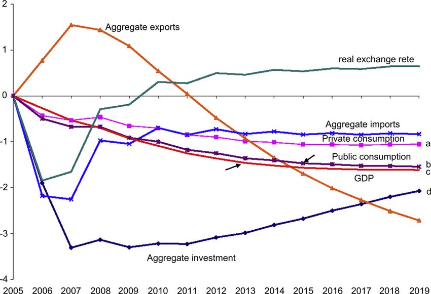
Figure 2.2 shows the deviations in the expenditure components of GDP. In the long
run these are all negative and range around that for GDP. The long-run deviations in
private consumption, public consumption and imports are less negative than that for
GDP while those for exports and investment are more negative than that for GDP.
We can understand these results as a sequence. The first element is that tighter border
security improves the US terms of trade. This is a benefit from having a 1.6% smaller
economy that demands less imports (thereby lowering their price) and supplies less
exports (thereby raising their price). The second element is that terms-of-trade
improvement allows private and public consumption to rise (as shown in Figure 2.2)
relative to GDP. This is because an improvement in the terms of trade increases the prices
of the goods and services produced by the US relative to prices of the goods and services
consumed by the US, allowing the US to sustain a higher level of consumption for any
given level of output (GDP).
The third element in understanding the long-run results in Figure 2.2 concerns
investment. In the very long run, the change in immigration policy that we are
considering will have little identifiable effect on the growth rate of labor input.
Consequently it will have little effect on the growth rate of capital and therefore on the
5 As will be explained shortly, there is a long-run increase in the terms of trade. Despite this, the cost of making a unit of
capital (which includes import prices but not export prices) does not fall relative to Pg (which includes export prices
but not import prices). This is mainly because in the long run the construction industry suffers an increase in its labor
costs relative to other industries reflecting its intensive use of unauthorized labor.32 Peter B. Dixon et al.
Figure 2.2 Expenditure aggregates with tighter border security (percentage deviations from
baseline).
ratio of investment to GDP.6 As can be seen in Figure 2.1, the deviation line for capital is
still falling slightly in 2019 indicating that the capital stock has not fully adjusted to the
1.6% reduction in labor input.7 With capital still adjusting downwards in 2019, the
investment to GDP ratio is still below its eventual long-run level. However, in terms of
contributions to GDP, the positive gaps in 2019 between the consumption and GDP
deviations outweigh the negative gap between the investment and GDP deviation (the
ac and bc gaps in Figure 2.2 weighted by private and public consumption easily
outweigh the dc gap weighted by investment). This explains why the long-run deviation
in imports in Figure 2.2 is less negative than that in exports.
The fourth element concerns the long-run relationships between the GDP deviation
and the trade deviations. Although we have now understood why Figure 2.2 shows
a long-run increase in imports relative to exports, we have not explained why these two
6 The rate of growth of capital is given by k ¼ (I/Y ) (Y/K ) e d, where I and Y are investment and GDP, and d is the
rate of depreciation (treated as a constant). Under our assumptions, the change in immigration policy does not affect k
or Y/K in the long run. Therefore, it does not affect I/Y.
7 It is apparent that the K/L ratio is heading to a slightly lower long-run value than in the baseline. This is because the
cost of making a unit of capital increases slightly in the long run relative to the price deflator for GDP, reflecting the
intensive use of unauthorized labor in the construction industry.The MONASH Style of Computable General Equilibrium Modeling: A Framework for Practical Policy Analysis 33
deviations straddle the GDP deviation. If a reduction in the supply of unauthorized
immigrants were particularly harmful (cost increasing) to export-oriented industries
then it would be possible for both the import and export deviation lines at 2019 to be
below that of GDP. Similarly, if a reduction in the supply of unauthorized immigrants
were particularly harmful to import-competing industries then it would be possible for
both the import and export deviation lines at 2019 to be above that of GDP. As shown in
Dixon et al. (2011), the long-run effects of reduced unauthorized immigration on the
industrial composition of activity are quite small, with no pronounced bias against or in
favor of either export-oriented or import-competing industries. The lack of bias is
a consequence of unauthorized employment being spread over many industries and
representing only a small share of costs in almost all industries. Thus, the required gap
between imports and exports is achieved with the import deviation line above that of
GDP in the long run and the export deviation line below that of GDP.
Two further points about the effects of reduced unauthorized immigration on trade
are worth noting. (i) The increase in imports relative to exports is in quantity terms.
With an improvement in the terms of trade there is no deterioration in the balance of
trade. (ii) The increase in imports relative to exports is facilitated, as shown in Figure 2.2,
by a long-run increase in the real exchange rate (an increase in the nominal exchange rate
relative to the foreign/US price ratio).
The final aspect of the long-run results in Figure 2.2 that we will explain is the
relative movements in public and private consumption. Public consumption falls relative
to private consumption because consumption of public goods by unauthorized immi-
grants is high relative to their consumption of private goods. In the baseline forecast for
2019, unauthorized immigrants account for 3.7% of public consumption, but only 2.4%
of private consumption.
The short-run results in Figure 2.2 are dominated by the need for the economy to
adjust to a lower capital stock than it had in the baseline forecast. In the short run, the
policy causes a relatively sharp reduction in investment. With US investment at the
margin being financed mainly by foreigners, a reduction in investment weakens demand
for the US dollar. Consequently, a reduction in investment weakens the US exchange
rate. This temporarily stimulates exports and inhibits imports. As the downward
adjustment in the capital stock is completed, investment recovers, causing the real
exchange rate to rise, exports to fall and imports to rise.
2.2.1.2 Effects on the occupational composition of legal employment
The starting point for the explanation of the long-run macroeconomic results was the
finding that a 28.7% cut in unauthorized employment reduces effective labor input
by 1.6%. But why 1.6? Recall that in the baseline forecast the share of the US wage
bill accounted for by unauthorized employment in 2019 is 3.64%. This suggests that
a 28.7% cut in unauthorized employment should reduce effective labor input by only34 Peter B. Dixon et al.
1.0% (¼ 3.64 0.287). The explanation of the discrepancy (1.0 versus 1.6) hinges on
changes in the occupational mix of legal US employment.
Table 2.1 gives occupational data for 2005 and deviation results for 2019. Column (1)
shows the share of unauthorized immigrants in the wage bill of each US occupation. The
occupational classification was chosen to give maximum detail on employment of
unauthorized immigrants, with about 90% of their employment being spread across the
first 49 occupations. The last occupation, ‘Services, other’, accounts for about 60% of US
employment, but only 10% of unauthorized employment. Columns (2) and (3) show the
long-run effects of the supply-restriction policy on employment and real wage rates of
legal US workers by occupation. In broad terms, the employment results in Table 2.1
show a long-run transfer of legal workers from ‘Services, other’, an amalgam of
predominantly high-skilled, high-wage jobs, to the occupations that currently employ
large numbers of unauthorized immigrants. The correlation coefficient between the
deviations in jobs for legal workers (column 2) and unauthorized shares (column 1) is
close to one. In occupations vacated by unauthorized immigrants, legal workers not only
gain jobs, but also benefit from significant wage increases. The correlation coefficient
between the employment and wage results in columns (2) and (3) is also close to one.
The long-run change in occupational mix implied by column (2) does not mean that
existing US workers change their occupations. For each occupation, restricting the
supply of unauthorized workers presents legal workers with opportunities to replace
unauthorized workers. On the other hand, the economy is smaller, generating a negative
effect on employment opportunities for legal workers. The positive replacement effect
dominates in the low-wage occupations that currently employ large numbers of unau-
thorized immigrants. The negative effect of a smaller economy dominates in high-wage
occupations that currently employ few unauthorized immigrants. Thus, there is an
increase in vacancies in low-wage occupations relative to high-wage occupations,
allowing low-wage occupations to absorb an increased proportion of new entrants to the
workforce and unemployed workers. Another way of understanding the change in the
occupation mix of legal workers is to recognize that the labor market involves job
shortages. At any time, not everyone looking for a job in a given occupation can find
a job in that occupation. So people settle for second best. The college graduate who
wants to be an economist settles for a job as an administrative officer; the high-school
graduate who wants to be a police officer settles for a job in private security; the
unemployed person who wants to be a chef settles for a job as a short-order cook; and so
on. Through this shuffling process, a reduction in supply of unauthorized immigrants
reduces the skill composition of employment of legal workers. It lowers the contribution
of these workers to effective labor input, explaining the 1.0 versus the 1.6 discrepancy.
We refer to this as a negative Occupation-mix effect. The idea of an Occupation-mix
effect will be familiar to students of the history of US immigration. As described by
Griswold (2002, p. 13), the inflow of low-skilled immigrants early in the twentiethThe MONASH Style of Computable General Equilibrium Modeling: A Framework for Practical Policy Analysis 35
Table 2.1 Occupational data for 2005 and deviation results for 2019
% deviation in 2019
Unauthorized immigrants:
% of labor costs in 2005 Legal jobs Legal real wage
Occupation (1) (2) (3)
1. Cooks 15.6 4.20 1.89
2. Grounds maintenance 24.8 7.45 3.19
3. House keeping and cleaning 22.0 6.56 2.82
4. Janitor and building cleaner 10.4 2.31 1.19
5. Miscellaneous agriculture worker 34.3 10.70 4.55
6. Construction laborer 23.9 7.10 3.16
7. Transport packer 24.6 7.37 3.19
8. Carpenter 15.1 3.90 1.92
9. Transport laborer 7.2 1.09 0.71
10. Cashier 4.7 0.31 0.43
11. Food serving 6.4 0.88 0.62
12. Transport driver 4.0 e0.09 0.25
13. Waiter 5.7 0.64 0.53
14. Production, miscellaneous assistant 8.3 1.07 0.72
15. Food preparation worker 13.3 3.42 1.61
16. Painter 24.9 7.46 3.31
17. Dishwasher 22.7 6.83 2.86
18. Construction, helper 24.8 7.42 3.30
19. Retail sales 2.4 e0.50 0.11
20. Production, helper 20.4 5.54 2.52
21. Packing machine operator 23.6 6.88 3.01
22. Butchers 21.0 6.20 2.74
23. Stock clerk 4.6 0.26 0.40
24. Child care 5.2 0.56 0.51
25. Miscellaneous food preparation 14.5 3.80 1.74
26. Dry wall installer 35.8 11.43 4.87
27. Nursing 2.8 e0.01 0.29
28. Industrial truck operator 8.5 1.47 0.87
29. Transport, cleaners 15.8 4.24 1.93
30. Automotive repairs 6.3 0.88 0.64
31. Sewing machine operator 18.8 4.95 2.39
32. Concrete mason 22.6 6.61 3.00
33. Roofers 28.2 8.64 3.78
34. Plumbers 7.1 1.07 0.80
35. Personal care 5.7 0.91 0.66
36. Shipping clerk 5.2 0.35 0.43
37. Brick mason 22.5 6.56 2.97
38. Carpet installer 21.4 6.21 2.82
39. Laundry 15.5 4.22 1.93
(Continued )36 Peter B. Dixon et al.
Table 2.1 Occupational data for 2005 and deviation results for 2019dcont'd
% deviation in 2019
Unauthorized immigrants:
% of labor costs in 2005 Legal jobs Legal real wage
Occupation (1) (2) (3)
40. Other production workers 9.1 1.57 0.91
41. Maintenance and repairs 2.2 e0.71 e0.01
42. Repair, helper 16.8 4.56 2.09
43. Welder 6.2 0.31 0.41
44. Supervisor, food preparation 3.4 e0.20 0.22
45. Construction supervisors 3.4 e0.27 0.27
46. Farm/food/clean, other 6.1 0.61 0.53
47. Construction, other 5.5 0.38 0.49
48. Production, other 4.6 e0.11 0.21
49. Transport, other 3.2 e0.40 0.13
50. Services, other 0.4 e1.27 e0.13
Total 2.6 e0.16 e0.46
century induced native-born US residents to complete their education and enhance their
skills. In our terms, that was a positive Occupation-mix effect.
Before leaving Table 2.1, it is worth commenting on the deviations shown in the
‘Total’ row. The reduction (0.16%) in employment of legal workers is caused by the shift
in the composition of their employment towards low-skilled occupations. These occu-
pations have relatively high equilibrium rates of unemployment, which we have assumed
are unaffected by immigration policy. It is sometimes asserted that cuts in employment of
unauthorized immigrants would reduce unemployment rates of low-skilled legal
workers. While our modeling suggests that there would be increases in the number of
jobs for legal workers in low-skilled occupations, this does not mean that unemployment
rates in these occupations would fall. With cuts in unauthorized immigration, low-skilled
legal workers might find themselves under increased pressure from higher-skilled workers
who can no longer find vacancies in higher-skilled occupations.
The overall reduction of 0.46% in the wage rate of legal workers seems surprising at
first glance. Column (3) of Table 2.1 shows an increase or a negligible decrease in wage
rates for legal workers in all occupations except ‘Services, other’ in which the wage rate is
reduced by 0.13%. However, the average hourly wage rate of legal workers is reduced by
the shift in the occupational composition of their employment to low-wage jobs.
2.2.1.3 Effects on the welfare of legal households
The headline number that policy makers are often looking for from a CGE study is the
effect on aggregate welfare. In the present study, we take this as referring to long-runThe MONASH Style of Computable General Equilibrium Modeling: A Framework for Practical Policy Analysis 37
Table 2.2 Long-run (2019) percentage effects of tighter border security on consumption of legal
residents
F1 Direct effect e0.29
F2 Occupation-mix effect e0.31
F3 Legal-employment effect e0.11
F4 Capital effect e0.24
F5 Public-expenditure effect 0.17
F6 Terms-of-trade effect 0.23
BOTE totals e0.55
CGE result e0.52
(2019) private and public consumption by legal US residents. We find that a reduction of
28.7% in unauthorized employment caused by tighter border security would generate
a sustained annual welfare loss for legal residents of 0.52% (about $80 billion in 2009
dollars).
This result can be explained in terms of the six factors indicated in Table 2.2 by
F1eF6. As detailed in Dixon et al. (2011), each of these factors can be quantified by
a BOTE calculation. The total of the BOTE calculations (e0.55) is an accurate estimate
of the CGE result (e0.52). This gives us confidence that we have adequately identified
the data and mechanisms in our model that explain the result. Here, we briefly describe
the factors and their quantification.
F1: Direct effect
With a reduction in supply, the wage rate of unauthorized workers will rise. This is
illustrated in Figure 2.3 in which DD is the demand curve for unauthorized labor in
2019, SS is the supply curve in the baseline forecast and S0 S0 is the supply curve with the
tighter security policy in place. The numbers shown in the diagram are taken from our
simulation: the policy reduces unauthorized employment in 2019 from 12.4 to 8.8
million and increases annual wage rates for unauthorized workers by 9.2%, from $52,660
to $57,500 (2019 dollars).
If workers are paid according to the value of their marginal product then the loss in
output (represented by GDP) from reducing employment is the change in the area under
the demand curve, area (abcd) in Figure 2.3. The change in the total cost to employers
of unauthorized immigrants is area (gaef), the increase in costs associated with the in-
crease in the unauthorized immigrant wage rate, minus area (ebcd), the reduction in
costs associated with employment of less unauthorized immigrants. Ignoring taxes, the
analysis so far suggests that the Direct effect of cutting illegal employment (the change in
GDP less the change in the costs of employing illegal workers) is a loss represented by
area (abfg). As indicated in Figure 2.3, this area is worth $51.5 billion. Taxes complicate
the situation in two ways. (i) The change in the area under the demand curve is an38 Peter B. Dixon et al.
Figure 2.3 Demand for and supply of illegal immigrants in 2019.
underestimate of the loss in GDP because indirect taxes mean that wage rates are less than
the value of the marginal product of workers. (ii) Unauthorized immigrants pay income
taxes. Consequently, area (ebcd) overstates the saving to the US economy associated
with paying wages to 28.6% fewer unauthorized immigrants and area (gaef) overstates
the cost to the US economy of paying higher wage rates to unauthorized immigrants
who remain in employment. After adjusting for taxes, the final estimate that Dixon et al.
(2011) obtained for the Direct effect was a loss of $77.3 billion. This causes a 0.29%
reduction in consumption by legal households (row 1, Table 2.2).
F2: Occupation-mix effect
Restricting the supply of unauthorized immigrants changes the occupational mix
of employment of legal workers, reducing their average hourly wage rate by 0.46% (Table
2.1). In the baseline forecast for 2019, wages are 66% of the total income of legal resi-
dents.8 A 0.46% reduction in average wage rates translates into a 0.31% (¼ 0.46 0.66)
reduction in the ability of legal residents to consume private and public goods.
8 This is GNP (i.e. GDP less net income flowing to foreign investors) minus post-tax income accruing to unauthorized
immigrant.The MONASH Style of Computable General Equilibrium Modeling: A Framework for Practical Policy Analysis 39 F3: Legal-employment effect As explained in Section 2.2.1.2, we assume that equilibrium rates of unemployment are higher for low-skilled occupations than for high-skilled occupations, leading in our simulation to a reduction in legal employment of 0.16% (Table 2.1). With wages being 66% of the total income of legal residents, this reduces their income and consumption by 0.11%. F4: Capital effect If a change in immigration policy had no effect on savings by legal residents (including the government) up to 2019, then it would have no effect on US ownership of capital in 2019. In this case, if a change in immigration policy led to a reduction in the stock of capital in the US, then it would lead to a corresponding reduction in the stock of foreign-owned capital, with little effect on capital income accruing to legal households. Nevertheless, they would suffer a welfare loss because the US treasury would lose taxes paid by foreign owners of US capital. Via the Direct effect and other negative effects in Table 2.1, the tighter border- security policy reduces saving by legal households throughout the simulation period. Thus, in the policy run, legal households own less US capital in 2019 than they had in the baseline forecast and lose the full-income of this lost capital. As explained in Section 2.2.1.1, the policy causes a long-run reduction in US capital stock of about 1.6%. This is split approximately evenly between reductions in foreign-owned and US-owned capital. Taking account of the tax effects of the loss of foreign-owned capital and the full-income effects of the loss of US-owned capital, we find that the 1.6% reduction in capital contributes e0.24% to sustained long-run welfare of legal households. F5: Public-expenditure effect With a reduction in the number of unauthorized immigrants working in the US, the public sector would cut its expenditures, particularly on elementary education, emer- gency healthcare and correctional services. This would allow either cuts in taxes or increased provision of public services to legal households. This effect contributes 0.17% to sustained long-run welfare of legal households.9 It should be noted that F5 encom- passes only public sector expenditures and does not take account of taxes paid by illegal immigrants. These taxes are accounted for in F1 where we compute the Direct contribution of illegal immigrants to GDP net of their post-tax wages. F6: Terms-of-trade effect In our simulation, the cut in unauthorized immigration reduces the prices of the goods and services that are consumed in the US relative to the prices of goods and services that 9 The underlying data on public expenditures on unauthorized immigrants were taken from Rector and Kim (2007) and Strayhorn (2006).
40   Peter B. Dixon et al.

     are produced in the US. In 2019, the policy-induced reduction in the price index for
     private and public consumption relative to that for GDP is 0.23%. This increases the
     consuming power of legal households by 0.23%. The main reason for the relative decline
     in the price of consumption is the improvement in the terms of trade, discussed in
     Section 2.2.1.1. A terms-of-trade improvement generally reduces the price index for
     consumption (which includes imports, but not exports) relative to that for GDP (which
     includes exports, but not imports).

     2.2.2 Engaging the audience: hoped-for reactions
     When we present a CGE story to an audience we are hoping for certain reactions. We
     want the audience to engage on the topic, not on prejudices and general views about
     CGE modeling. Whether we get the desired reaction depends on how well we have told
     the story in terms of mechanisms that are accessible to people without a CGE
     background.
          In the case of our tighter border-security story, we hope that the audience is
     enthusiastic enough to want to know about extensions. For example, what would
     happen if the reduction in unauthorized employment were achieved by restricting
     demand through more rigorous prosecution of employers rather than restricting supply?
     More radically, what would happen if we replaced unauthorized immigrants by low-
     skilled guest workers? If we have told our story sufficiently well then audiences or readers
     of our papers can go a long way towards answering these questions without relying on
     our model.
          The effects of demand restriction can be visualized in terms of Figure 2.3 as an inward
     movement in DD rather than SS. If the demand policy were scaled to achieve the same
     reduction in unauthorized employment as in the supply policy, then we would expect
     similar results for F2eF6. which depend primarily on the reduction in the number of
     unauthorized workers. At first glance we might expect the Direct effect (F1) for
     demand-side restriction to be more favorable than that for supply-side restriction: with
     demand-side restriction, wage rates for unauthorized workers fall rather than rise.
     However, when we think of the gap between the supply-restricted wage (da in
     Figure 2.3) and the demand-restricted wage (dh) as being absorbed by prosecution-
     avoiding activities, then we can conclude that even the Direct effect will be similar under
     the demand- and supply-side policies. Thus, on the basis of F1eF6 we would expect
     little difference in the effects of equally scaled demand- and supply-side policies. This is
     confirmed in Dixon et al. (2011).
          The guest-worker question arose from comments by Dan Griswold of the Cato
     Institute (a free-trade think tank in Washington, DC). After seeing a presentation on the
     negative welfare result in Table 2.2, he asked whether welfare would increase if there
     were more low-skilled immigrants employed in the US rather than less. This led to
     a consideration of a program under which US businesses could obtain permits to legally
The MONASH Style of Computable General Equilibrium Modeling: A Framework for Practical Policy Analysis 41
employ low-skilled immigrants. In terms of Figure 2.3, we can envisage such a program
as shifting the supply curve outward e at any given wage, more low-skilled immigrants
would be willing to enter the US under a guest-worker program than under the present
situation in which they incur considerable costs from illegal entry. The outward shift in
the supply curve would reverse the signs of the six effects identified in Table 2.2. As
shown in Dixon and Rimmer (2009), a permit charge paid by employers could be used
to control the number of low-skilled immigrants. It would also be a useful source of
revenue, effectively transferring to the US treasury what are currently the costs to
immigrants of illegal entry.
A second hoped-for reaction from audiences is well-directed questions about
robustness and sensitivity. By this we mean questions about data items and parameter
values that can be identified from our story as being important for our results. In
presentations of our work on unauthorized immigration, we welcome questions con-
cerning: our baseline forecasts for unauthorized employment (7.3 million in 2005
growing to 12.4 million in 2019); our data on the occupational and industrial compo-
sition of unauthorized and legal employment; our assumptions about the level of public
expenditures associated with unauthorized employment; our choice of values for the
elasticities of demand and supply for unauthorized workers; our adoption of a one-
country framework that ignores effects outside the US; and other key ingredients of our
story. When questions are asked about the existence, uniqueness and stability of
competitive equilibria, then we suspect that our presentation has not effectively led the
audience to understand how they should assess what we are saying.
A third satisfying reaction is curiosity about results for other dimensions. In our story
here we have concentrated on macro and occupational results but for an interested
audience we could also report industry results: our simulations were conducted at a 38-
industry level. Greater industrial disaggregation can be introduced for organizations with
a particular industry focus. For example, in a current study on unauthorized workers in
agriculture, the US Department of Agriculture has expanded the industrial dimension to
70, emphasizing agricultural activities.
For readers of this chapter, we hope that our story has done two things. (i) We hope
that it has demonstrated how CGE results can be explained in non-circular, macro-to-
micro fashion. As in this story, we have found that in explaining most CGE results the
best starting point is the inputs to the aggregate production function. In this case we
started with what a cut in unauthorized immigration would do to aggregate employ-
ment. We then moved to the effect on aggregate capital. From there we went to the
expenditure side of GDP. Eventually we worked down to employment by occupation.
(ii) We hope that our story has aroused curiosity about some methodological issues. We
have mentioned the business-as-usual forecast or baseline. How is this created in
a MONASH model? We have reported policy-induced deviations. How are policy
simulations conducted and what is their relationship to baseline simulations? We have42 Peter B. Dixon et al.
worked with considerable labor market disaggregation: 50 occupations by two birth-
places by two legal statuses by 38 industries. How do we cope with large dimensions? We
have shown year-by-year results. How do we handle dynamic mechanism such as capital
accumulation that provide connections between years?10 These are among the issues
discussed in the rest of this chapter.
2.3 FROM JOHANSEN TO ORANI
Modern CGE modeling has not evolved from a single starting point and there are still
quite distinct schools of CGE modeling. While Johansen (1960) made the first CGE
model, there were several other largely independent starting points including the
contributions of Scarf (1967, 1973), Jorgenson and associates (e.g. Hudson and
Jorgenson, 1974) and the World Bank group (e.g. Adelman and Robinson, 1978; Taylor
et al., 1980). Each of these later contributors adopted a style quite distinct from that of
Johansen: different computational techniques, estimation methods, approaches to result
analysis and issue focuses. In the case of the MONASH models, the ancestor is Johansen.
His style was simple, effective and adaptable. It facilitated the inclusion of policy-relevant
detail in CGE models and opened a path to result interpretation via BOTE explanations.
In this section we describe Johansen’s model and the extensions that were made in
creating the ORANI model.
2.3.1 Johansen model
Johansen presented his 22-commodity/20-industry model of Norway as a system of 86
linear equations connecting 86 endogenous and 46 exogenous variables:
AX x þ AY y ¼ 0; (2.2)
where x and y are 46 1 and 86 1 vectors of exogenous and endogenous variables, and
AX and AY are matrices of coefficients of dimensions 86 46 and 86 86 built mainly
from Norwegian input-output data for 1950 supplemented by estimates of income
elasticities for consumer demand.
The 46 exogenous variables are: aggregate employment (1); aggregate capital (1);
population (1); Hicks-neutral primary factor technical change in each industry (20);
exogenous demand for each commodity (22); and the price of non-competing imports
(1).11 The 86 endogenous variables are: labor input and capital input by industry
(2 20); output and prices by commodity (2 22); the average rate of return on capital
10 For dynamic mechanisms that are specific to our immigration work, such as vacancy-induced occupational shuffling,
we refer readers to Dixon and Rimmer (2010a).
11 We are sometimes asked about the numéraire in Johansen’s model. It is the nominal wage rate which is exogenously
fixed on zero growth and then omitted from the model.The MONASH Style of Computable General Equilibrium Modeling: A Framework for Practical Policy Analysis 43
(1); and aggregate private consumption (1). All of the variables in Johansen’s system are
growth rates or percentage growth rates. Johansen derived the equations in (2.2) from
underlying levels forms. For example, in (2.2) he represented the CobbeDouglas
relationship:
g
Zj ¼ Nj j Kj j e3j t ;
b
(2.3)
between the output in industry j (Zj) and labor and capital inputs (Nj and Kj) as:
zj gj nj bj kj ej ¼ 0; (2.4)
where zj, nj and kj are percentage growth rates in Zj, Nj and Kj, and ej is the rate of
technical progress.
From (2.2) Johansen solved his model, i.e. expressed growth rates in endogenous
variables in terms of exogenous variables, as:
y ¼ b x; (2.5)
where b is the 86 46 matrix given by:
b ¼ A1
Y AX : (2.6)
Johansen was fascinated by the b matrix in (2.6) and devoted much of his book to
discussing it. The b matrix shows the sensitivity (usually an elasticity) of every endog-
enous variable with respect to every exogenous variable. Johansen regarded the 3956
entries in the b matrix as his basic set of results and he looked at every one of them. His
management strategy for coping with 3956 results was to use a simple one-sector BOTE
model as a guide. The BOTE model told him what to look for and what to expect in his
full-scale model.
For example, the BOTE model suggested that the entries in the b matrix referring to
the elasticities of industry outputs with respect to movements in aggregate capital and
labor should lie in the (0,1) interval. This follows from a macro version of equation
(2.4).12 With one exception, this expectation was fulfilled: the b matrix shows a negative
entry for the elasticity of equipment output with respect to an increase in aggregate
employment. Following up and explaining exceptions is an important part of the BOTE
methodology. In this way we can locate result-explaining mechanisms in the full model
that are not present in the BOTE model. In other words, we can figure out what the full
model knows that the BOTE model does not know. In the case of the equipment-
output/employment elasticity, the explanation of the negative result is that an increase in
aggregate employment changes the composition of the economy’s capital stock in favor
of structures and against equipment. This morphing of the capital stock reduces
12 That is z ¼ g n þ b k þ e, where g and b are parameters with values between 0 and 1.44 Peter B. Dixon et al.
maintenance demand for equipment, thereby reducing the output of the equipment
industry.13
One of the most interesting parts of b is the submatrix relating movements in industry
outputs to movements in exogenous demands. At the time when Johansen was writing,
Leontief’s input-output model, with its emphasis on input-output multipliers, was the
dominant tool for quantitative multisectoral analysis. In Leontief ’s model, if an extra unit of
output from industry j is required by final users, then production in j must increase by at
least one unit and production in other industries will increase to provide intermediate
inputs to production in j. Further rounds of this process can be visualized with suppliers to j
requiring extra intermediate inputs. Thus, in Leontief ’s picture of the economy, developed
in the depressed 1930s,14 industries are in a complementary relationship, with good news
for any one industry spilling over to every other industry. Johansen, working in the
booming 1950s challenged this orthodoxy. His industry-output/exogenous-demand
submatrix implies diagonal effects that in most cases are less than one and off-diagonal
effects and are predominantly negative. Rather than emphasizing complementary
relationships between industries, Johansen emphasized competitive relationships. In
Johansen’s model, expansion of output in one industry drags primary factors away from
other industries. Only where there are particularly strong input-output links did Johansen
find that stimulation of one industry (e.g. food) benefits another industry (e.g. agriculture).
Having examined the b matrix, Johansen used it to decompose movements in
industry outputs, prices and primary factor inputs into parts attributable to observed
changes in exogenous variables. In making his calculations he shocked all 46 exogenous
variables with movements representing average annual growth rates for the period
around 1950. In discussing the results of his decomposition exercise, Johansen paid
particular attention to agricultural employment. This was a contentious issue among
economists in 1960. On the one hand, diminishing returns to scale suggested that relative
agricultural employment would grow with population and perhaps even with income
despite low expenditure elasticities for agricultural products. On the other hand, agri-
culture was experiencing rapid technical progress, suggesting that employment in
agriculture might not only fall as a share of total employment but might even fall in
absolute terms. Johansen was able to separate and quantify these conflicting forces. He
found that growth in capital, employment and population around 1950 caused relatively
strong increases in agricultural employment, consistent with diminishing returns to scale
interacting with increased consumption of food. However, the dominant effect on
agricultural employment was technical change. This was strongly negative, leaving
agriculture with net declining employment.
13 For a fuller explanation of Johansen’s negative equipment-output/employment elasticity, see Dixon and Rimmer
(2010c, p. 7).
14 Leontief (1936).You can also read