Surface Atmosphere Integrated Field Laboratory (SAIL) Science Plan
←
→
Page content transcription
If your browser does not render page correctly, please read the page content below
DOE/SC-ARM-21-004

Surface Atmosphere Integrated Field Laboratory
(SAIL) Science Plan

D Feldman           A Aiken
W Boos              R Carroll
V Chandrasekar      W Collins
S Collis            J Deems
P DeMott            J Fan
A Flores            D Gochis
J Harrington        M Kumijian
LR Leung            T O’Brien
M Raleigh           A Rhoades
S McKenzie Skiles   J Smith
R Sullivan          P Ullrich
A Varble            K Williams

April 2021
DISCLAIMER

This report was prepared as an account of work sponsored by the U.S.
Government. Neither the United States nor any agency thereof, nor any of
their employees, makes any warranty, express or implied, or assumes any
legal liability or responsibility for the accuracy, completeness, or
usefulness of any information, apparatus, product, or process disclosed, or
represents that its use would not infringe privately owned rights. Reference
herein to any specific commercial product, process, or service by trade
name, trademark, manufacturer, or otherwise, does not necessarily
constitute or imply its endorsement, recommendation, or favoring by the
U.S. Government or any agency thereof. The views and opinions of
authors expressed herein do not necessarily state or reflect those of the
U.S. Government or any agency thereof.

This report was produced by the Surface Atmosphere Integrated Field
Laboratory (SAIL) science team. It is a review of the science goals for the
SAIL campaign and the proposed strategies for addressing these goals.
The Atmospheric Radiation Measurement (ARM) user facility is working
closely with the SAIL science team to support these science goals;
however, implementation details may evolve during the course of the
campaign planning and execution.

This report is available on the U.S. Department of Energy Office of
Scientific and Technical Information website, osti.gov, and the ARM user
facility website, arm.gov.
DOE/SC-ARM-21-004

Surface Atmosphere Integrated Field
Laboratory (SAIL) Science Plan

D Feldman, Lawrence Berkeley National Laboratory (LBNL)
Principal Investigator

A Aiken, Los Alamos National Laboratory
W Boos, University of California, Berkeley
R Carroll, Desert Research Institute
V Chandrasekar, Colorado State University (CSU)
W Collins, LBNL
S Collis, Argonne National Laboratory (ANL)
J Deems, National Snow and Ice Data Center
P DeMott, CSU
J Fan, Pacific Northwest National Laboratory (PNNL)
A Flores, Boise State University
D Gochis, National Center for Atmospheric Research
J Harrington, Pennsylvania State University (PSU)
M Kumijian, PSU
LR Leung, PNNL
T O’Brien, Indian University
M Raleigh, Oregon State University
A Rhoades, LBNL
S McKenzie Skiles, University of Utah
J Smith, University of California, Irvine
R Sullivan, ANL
P Ullrich, University of California, Davis
A Varble, PNNL
K Williams, LBNL
Co-Investigators

April 2021

Prepared for the U.S. Department of Energy,
Office of Science, Biological and Environmental Research Program
D Feldman et al., April 2021, DOE/SC-ARM-21-004

                                    Executive Summary
Mountains are the natural water towers of the world, effectively turning water vapor into readily available
fresh water through precipitation, snowpack, and runoff. Unfortunately, Earth system models (ESMs)
have persistently been unable to predict the timing and availability of water resources from mountains
because the source(s) of model error are difficult to isolate in complex terrain with limited atmospheric or
land-surface observations. Further complications arise from the gross scale mismatch between ESM grid
box sizes and the relevant scales of mountainous hydrological processes. The mountain
hydrometeorology community has repeatedly called for integrated atmospheric and land observations of
water and energy budgets in complex terrain that span these scales to establish benchmarks against which
scale-dependent models can be further developed.

The Surface Atmosphere Integrated field Laboratory (SAIL) campaign responds to these calls by
deploying the U.S. Department of Energy (DOE) Atmospheric Radiation Measurement (ARM) user
facility’s second Mobile Facility (AMF2), additional ARM instrumentation, and an X-band scanning
precipitation radar from Colorado State University to the East River Watershed near Crested Butte,
Colorado. Integrated observations are key to the success of the SAIL campaign. Therefore, SAIL will
collocate atmospheric observations with the long-standing collaborative resources including the ongoing
surface and subsurface hydrologic observations from the DOE’s Watershed Function Science Focus Area
(SFA). It will also work closely with the U.S. Geological Survey (USGS) as part of its Next-Generation
Water Observing System (NGWOS), the National Oceanic and Atmospheric Administration (NOAA)’s
Study of Precipitation and Lower-Atmospheric impacts on Streamflow and Hydrology (SPLASH), and
the Rocky Mountain Biological Laboratory.

SAIL’s main science question is: Across a range of models from LES to mesoscale process to Earth
system models, what level of atmospheric and land-atmosphere interaction process fidelity is needed to
produce unbiased seasonal estimates of the surface energy and water budgets of mountainous watersheds
in the Upper Colorado River Basin?

In order to answer that question, SAIL will collect data to address four key science sub-questions:
1. SSQ-1. How do multi-scale dynamic and microphysical processes control the spatial and temporal
   distribution, phase, amount, and intensity of precipitation?
2. SSQ-2. How strongly do aerosols affect the surface energy and water balance by altering clouds,
   precipitation, and surface albedo, and how do these impacts vary seasonally?
3. SSQ-3. What are the contributions of snow sublimation, radiation, and turbulent fluxes of latent and
   sensible heat to the water and energy balance of the snowpack?
4. SSQ-4. How do atmospheric and surface processes set the net radiative absorption that is known to
   drive the regional flow of water into the continental interior during the summer monsoon?

SAIL data will enable the quantification of the processes that need to be represented at the scale of
mountainous watersheds, to help build a foundation for the robust process modeling required to advance
the representation of mountain hydrology in ESMs.

                                                       iii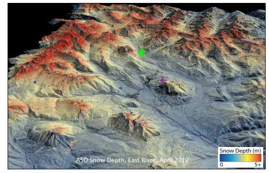
D Feldman et al., April 2021, DOE/SC-ARM-21-004

The campaign will start on September 1, 2021 and end on June 15, 2023, allowing for observations of
precipitation, aerosol, cloud, radiative, and surface processes as they impact mountainous hydrology
across multiple seasonal cycles.

                                                     iv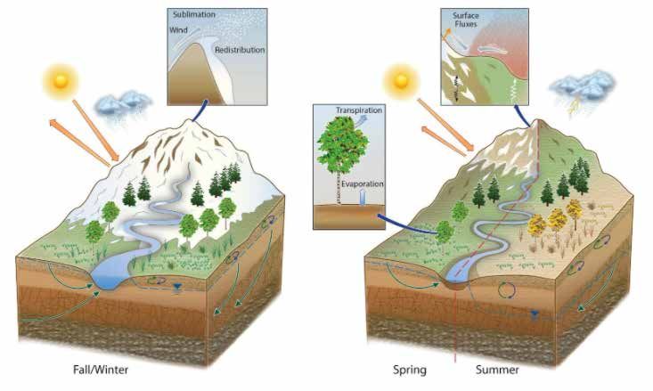
D Feldman et al., April 2021, DOE/SC-ARM-21-004

                Acronyms and Abbreviations
3D           three-dimensional
ABL          atmospheric boundary layer
ACSM         aerosol chemical speciation monitor
AERI         atmospheric emitted radiance interferometer
AERIOE       Atmospheric Emitted Radiance Interferometer Optimal Estimation Value-Added
             Product
AGL          above ground level
AMF          ARM Mobile Facility
AOP          Aerosol Optical Properties Value-Added Product
AOS          Aerosol Observing System
AOSMET       AOS meteorological measurements
APS          aerodynamic particle sizer
ARM          Atmospheric Radiation Measurement
ASD          Analytical Spectral Devices
ASFS         Atmospheric Surface Flux Station
ASO          Airborne Snow Observatory
ASR          Atmospheric System Research
BC           black carbon
BCSD-CMIP5   Bias-Corrected, Spatially Disaggregated downscaled Coupled Model
             Intercomparison Project – Phase 5
BER          Biological and Environmental Research
BERAC        Biological and Environmental Research Advisory Committee
BL           boundary layer
BrC          brown carbon
CASTNET      Clean Air Status and Trends Network
CB           cloud base
CBAC         Crested Butte Avalanche Center
CBMR         Crested Butte Mountain Resort
CCN          cloud condensation nuclei, cloud condensation nuclei particle counter
CEIL         ceilometer
CERES        Clouds and the Earth’s Radiant Energy System
CIES         column-integrated energy source
CLAMPS       Collaborative Lower Atmospheric Mobile Profiling System
CO           carbon monoxide, carbon monoxide mixing ration system
CONUS        continental United States
CPC          condensation particle counter

                                           v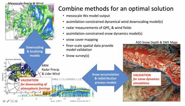
D Feldman et al., April 2021, DOE/SC-ARM-21-004

CPCF       condensation particle counter-fine
CSPHOT     Cimel sunphotometer
CSU        Colorado State University
CWCB       Colorado Water Conservation Board
CWP        cloud water path
DEM        digital elevation model
DL         Doppler lidar
DLPROF     Doppler Lidar Profiles Value-Added Product
DOE        U.S. Department of Energy
DSM        digital soil mapping
EC         eddy covariance
ECOR       eddy correlation flux measurement system
EDW        elevation-dependent warming
EESM       Earth and Environmental System Modeling
EESSD      Earth and Environmental Systems Sciences Division
EM         electromagnetic
EPA        Environmental Protection Agency
ESM        Earth system model
ESS        Environmental System Science
ET         evapotranspiration
EVI        enhanced vegetation index
FT         free troposphere
GNDRAD     ground radiometer on stand for upwelling radiation
GPM        Global Precipitation Measurement
HRRR       High-Resolution Rapid Refresh
HSRL       high-spectral-resolution lidar
HTDMA      humidified tandem differential mobility analyzer
IFL        integrated field laboratory
IMPROVE    Interagency Monitoring of Protected Visual Environments
INP        ice-nucleating particle
IOP        intensive operational period
IRT        infrared thermometer
IWP        ice water path
JPL        Jet Propulsion Laboratory
KAZR       Ka-band ARM Zenith Radar
LAI        leaf area index
LBNL       Lawrence Berkeley National Laboratory
LDQUANTS   Laser Disdrometer Quantities Value-Added Product

                                         vi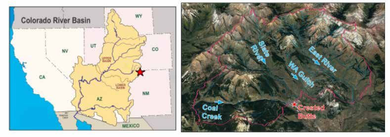
D Feldman et al., April 2021, DOE/SC-ARM-21-004

LES        large-eddy simulation
LIDAR      light detection and ranging
MARCUS     Measurements of Aerosols, Radiation, and Clouds over the Southern Ocean
MASL       meters above sea level
MERRA-2    Modern-Era Retrospective analysis for Research Applications, Version 2
MET        surface meteorological instrumentation
MFRSR      multifilter rotating shadowband radiometer
MFRSRCOD   Multifilter Rotating Shadowband Radiometer Cloud Optical Depth Value-Added
           Product
MODIS      Moderate Resolution Imaging Spectroradiometer
MPL        micropulse lidar
MT-CLIM    Mountain Climate Simulator
MWR        microwave radiometer
MWR3C      microwave radiometer, 3-channel
MWRLOS     Microwave Water Radiometer: Water Liquid and Vapor along Line of Sight Path
           Value-Added Product
NADP       National Atmospheric Deposition Program
NAM        North American Monsoon
NAME       North American Monsoon Experiment
NARCCAP    North American Regional Climate Change Assessment Program
NASA       National Aeronautics and Space Administration
NCAR       National Center for Atmospheric Research
NCP        normalized coherent power
NDVI       normalized difference vegetation index
NEON       National Ecological Observatory Network
NEPH       nephelometer
NGWOS      Next-Generation Water Observing System
NOAA       National Oceanic and Atmospheric Administration
NOHRSC     National Operational Hydrologic Remote Sensing Center
NPF        new particle formation
NSF        National Science Foundation
OACOMP     Organic Aerosol Component Value-Added Product
OZONE      ozone monitor
PARS2      Parsivel2 disdrometer
PBL        planetary boundary layer
PCASP      passive cavity aerosol spectrometer
PH         Pumphouse
POPS       printed optical particle spectrometer

                                         vii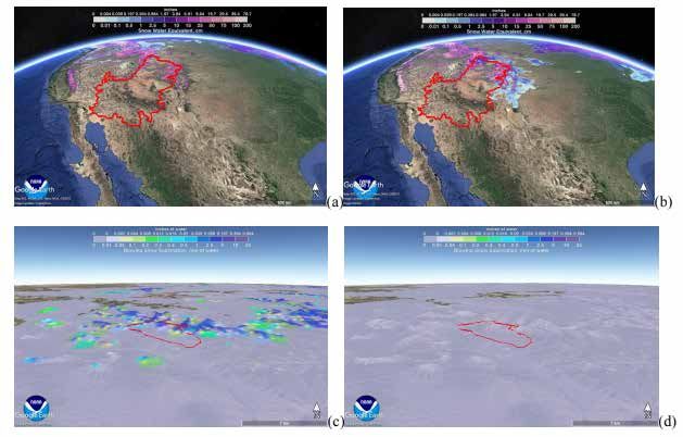
D Feldman et al., April 2021, DOE/SC-ARM-21-004

PPI           plan-position indicator
PRISM         Parameter-Elevation Regressions on Independent Slopes Model
PSAP          particle soot absorption photometer
QCECOR        Quality-Controlled Eddy Correlation Measurement Value-Added Product
RADFLUXANAL   Radiative Flux Analysis Value-Added Product
RADSYS        radiometer suite
RGB           red, green, blue
RGMA          Regional & Global Model Analysis
RHI           range-height indicator
RMBL          Rocky Mountain Biological Laboratory
RWP           radar wind profiler
SAIL          Surface Atmosphere Integrated Field Laboratory
SBR           Subsurface Biogeochemical Research
SEB           surface energy balance
SEBS          surface energy balance system
SFA           Science Focus Area
SKYRAD        sky radiometers on stand for downwelling radiation
SLR           Snow-Level Radar
SMPS          scanning mobility particle sizer
SNICAR        Snow-Ice and Aerosol Radiative Transfer
SNOTEL        Snow Telemetry
SO            science objective
SOA           secondary organic aerosol
SONDE         balloon-borne sounding system
SP2           single-particle soot photometer
SPLASH        Study of Precipitation and Lower-Atmospheric impacts on Streamflow and
              Hydrology
SQ            science question
SSQ           science sub-question
STAC          size- and time-resolved aerosol counter
STORMVEX      Storm Peak Lab Cloud Property Validation Experiment
SURFRAD       Surface Radiation Network
SWE           snow-water equivalent
TBS           tethered balloon systems
TES           Terrestrial Ecosystem Science
TOA           top-of-atmosphere
TRMM          Tropical Rainfall Measuring Mission
TSI           total sky imager

                                           viii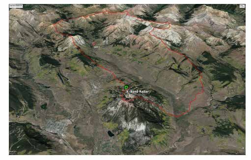
D Feldman et al., April 2021, DOE/SC-ARM-21-004

UAV         unmanned aerial vehicle
UHSAS       ultra-high-sensitivity aerosol spectrometer
USGS        U.S. Geological Survey
VAP         Value-Added Product
VARANAL     Constrained Variational Analysis Value-Added Product
VR-CESM     Variable-Resolution Community Earth System Model
WBPLUVIO2   Pluvio2 weighing bucket rain gauge
WFSFA       Watershed Function Scientific Focus Area
WRF         Weather Research and Forecasting
WU          Weather Underground
WUS         Western United States
XBPWR       X-band dual-polarimetric weather radar

                                          ix
D Feldman et al., April 2021, DOE/SC-ARM-21-004
Contents
Executive Summary ..................................................................................................................................... iii
Acronyms and Abbreviations ....................................................................................................................... v
1.0 Background........................................................................................................................................... 1
1.1 Campaign Overview..................................................................................................................... 4
1.2 Previous Campaigns ................................................................................................................... 14
1.2.1 STORMVEX ................................................................................................................... 14
1.2.2 NAME ............................................................................................................................. 15
2.0 Scientific Questions ............................................................................................................................ 16
2.1 Precipitation Processes ............................................................................................................... 16
2.2 Aerosol Processes....................................................................................................................... 19
2.3 Snow Processes .......................................................................................................................... 22
2.4 Warm-Season Processes............................................................................................................. 25
3.0 Scientific Objectives ........................................................................................................................... 26
3.1 Precipitation Process Characterization ....................................................................................... 27
3.2 Cold Snow-Season Processes ..................................................................................................... 28
3.3 Aerosol Regimes and Radiation ................................................................................................. 30
3.4 Aerosol-Cloud Interactions ........................................................................................................ 33
3.5 Surface Energy Balance ............................................................................................................. 34
4.0 Measurement Strategies ...................................................................................................................... 36
4.1 AMF2 and XBPWR during Normal Operations ........................................................................ 39
4.1.1 Strategies Supporting Science Objective 1...................................................................... 40
4.1.2 Strategies Supporting Science Objective 2...................................................................... 41
4.1.3 Strategies Supporting Science Objective 3...................................................................... 42
4.1.4 Strategies Supporting Science Objective 4...................................................................... 43
4.1.5 Strategies Supporting Science Objective 5...................................................................... 43
4.2 Collaborative Resources and Guest Instrumentation ................................................................. 44
4.3 Other ARM Resources ............................................................................................................... 45
5.0 Project Management and Execution ................................................................................................... 47
6.0 Science ................................................................................................................................................ 48
6.1 Precipitation Process Science ..................................................................................................... 48
6.2 Snow Sublimation and Wind Redistribution Science ................................................................ 49
6.3 Aerosol Precipitation Interaction Science .................................................................................. 51
6.4 Surface Energy Balance Science ................................................................................................ 52
6.5 Integrated Field Laboratory Science .......................................................................................... 52
6.6 Modeling Activities Science ...................................................................................................... 53
7.0 Relevancy to the DOE Mission .......................................................................................................... 55
8.0 References .......................................................................................................................................... 56
xD Feldman et al., April 2021, DOE/SC-ARM-21-004
Figures
1 Cartoon of the dominant atmospheric and surface processes in mid-latitude continental interior
mountainous watersheds that impact mountainous hydrology and their interseasonal variability......... 3
2 The 640,000 km2 Colorado River Watershed and, on the right, the 300 km2 drainage that
includes Coal Creek, the Slate River, Washington Gulch and the East River located within 20 km
of Crested Butte, Colorado. .................................................................................................................... 4
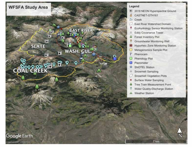
3 Watershed boundaries of Coal Creek, Slate River, Washington Gulch, and the East River, along
with tributary overlays............................................................................................................................ 5
4 Map of the East River Watershed depicting the network of stream gauging/stream water
sampling locations, meteorological stations, and other distributed and specialized measurement
sites in the watershed. ........................................................................................................................... 13
5 Seasonal cycle and range of interannual variability of monthly-mean GPCC (v7) precipitation
over a 1x1-degree box centered on Crested Butte (left), and over the entire Colorado-Utah region
(right). ................................................................................................................................................... 14
6 1981-2010 climatological average of the seasonal trajectory in measured total precipitation and
snow-water equivalent at the Butte and Schofield Pass SNOTEL stations as a function of day in
water year. ............................................................................................................................................ 14
7 Info-graphic showing precipitation micro- and macro-physical processes that contribute to
precipitation in high-altitude complex terrain. ..................................................................................... 17
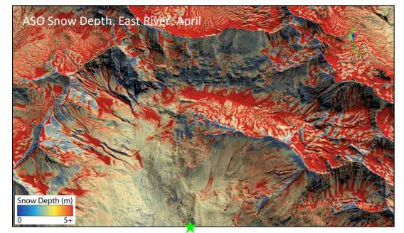
8 ASO-measured snow depth around Crested Butte, Colorado in early April, 2019. ............................. 18
9 Cartoon of a range of aerosol processes that impact radiation and precipitation and, ultimately,
hydrology.............................................................................................................................................. 19
10 Diagram of range of atmospheric aerosol processes and their impacts. ............................................... 21
11 Annual cycles of aerosol mass concentrations of fine organic and elemental carbon, and soil
dust, at the White River Interagency Monitoring of Protected Visual Environments (IMPROVE)
network site, located close to the proposed SAIL site, at 3413 m MSL, 39.1536 latitude, -
106.8209 longitude. (b) INP concentrations via immersion freezing collected by several
campaigns since 2000 in the Colorado Mountains. .............................................................................. 22
12 ASO Snow Water Equivalent Retrieval Comparison over the East River Watershed from (left)
April 1, 2016, (center) March 30, 2018, and (right) May 24, 2018...................................................... 23
13 Box-whisker plots (box spans 25-75th percentile and whiskers span the 5th to 95th percentiles)
of ASO SWE as a function of elevation bin. ........................................................................................ 23
14 Cartoon of three major areas where snow sublimation occurs: Over the snowpack, in the canopy,
and at ridgelines in blowing snow plumes............................................................................................ 24
15 NOHRSC estimates of (a) April 1, 2020 SWE, (b) April 1, 2019 SWE, (c) April 1, 2020
blowing-snow sublimation and (d) April 1, 2019 blowing-snow sublimation. .................................... 25
16 Climatological June-August atmospheric column-integrated energy source, obtained by
summing the surface sensible and latent heat flux and the column-integrated radiative flux
convergence, as estimated from MERRA-2 reanalysis. ....................................................................... 26
xiD Feldman et al., April 2021, DOE/SC-ARM-21-004
17 XBPWR beam-blockage analysis from the Old Teocali Lift site showing radial coverage in (a)
winter and (b) summer.......................................................................................................................... 28
18 Panoramic drone photo of Old Teocali Lift site looking towards Gothic, Colorado............................ 28
19 ASO survey of the northern edge of the East River Watershed from April, 2019 showing
variability of snowpack near ridgelines. ............................................................................................... 29
20 Map of the radiative forcing by deposited aerosols in snow from the ASO flight over the East
River Watershed in April, 2016............................................................................................................ 31
21 Diagram of impacts of impurities on the surface albedo of snow and associated snow-albedo and
grain-size feedbacks. ............................................................................................................................ 33
22 Cartoon of range of aerosol-precipitation processes with the relative vertical positioning in the
atmosphere and their length scales. ...................................................................................................... 34
23 Perspective view looking north towards East River Watershed with the watershed boundary in
red, the location for SAIL of the XBPWR in green, and the location of the AMF2 as a red
marker................................................................................................................................................... 40
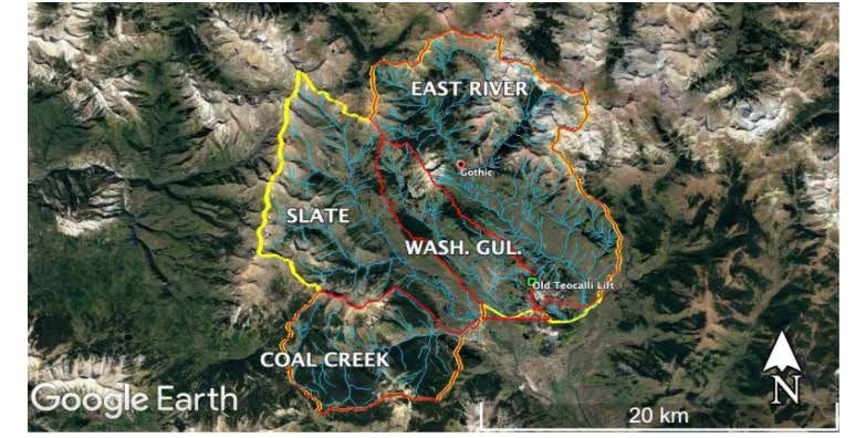
24 Three potential sites for TBS deployment: (1) RMBL Gothic Townsite in red, Kettle Ponds in
yellow, and Mt. Crested Butte Boneyard in yellow. ............................................................................ 46
25 (a) Topographic map of a 400x400-km domain surrounding the East River Watershed (outlined
in black). (b) Domain-wide comparison of wintertime WRF simulations with PRISM for
Calendar Year 2017. (c) Same as (b) but showing wintertime domain bias (WRF-Prism), (d)
Same as (c) but showing summertime bias. ......................................................................................... 48
26 Two-pronged data assimilation to achieve snow process closure at the mesoscale. ............................ 50
27 Example of determination of biological INPs based on thermal treatment of unamended aliquots
of particles, and distinguishing total organic contributions of INPs through H2O2 digestion. ............. 51
Tables
1 List of SAIL AOS instruments including summary information. .......................................................... 7
2 List of SAIL cloud instruments including summary information. ......................................................... 8
3 List of SAIL wind instruments including summary information. .......................................................... 8
4 List of SAIL radiometry instruments including summary information. ................................................. 9
5 List of SAIL surface meteorology instruments including summary information................................. 10
xiiD Feldman et al., April 2021, DOE/SC-ARM-21-004
1.0 Background
The majority of worldwide water resources (60-90%) emerge from mountains (Huss et al. 2017). In North
America, mountains comprise a quarter of the continent’s land area, but store 60% of the snowpack
(Wrzesien et al. 2018). However, these water towers of the world are threatened by many factors
contributing to elevation-dependent climate warming (Barnett et al. 2005, Mote et al. 2018, MRI 2015,
López-Moreno et al. 2017, Musselman et al. 2017), with deleterious implications for snow cover, water
resources, and even atmospheric dynamics (Chen et al. 2017, MRI 2015, Mote et al. 2018). This warming
is expected to induce modifications to snow accumulation, melt, and subsequent water budget partitioning
and is expected to decrease streamflow (Clow 2010, Barnhart et al. 2016, Li et al. 2017,
McCabe et al. 2017). Given the potential for water resource stress in the near and long term, there are
clear societal needs for Earth system models (ESMs) to provide robust predictions of how water resources
arising from, especially, mid-latitude mountain systems will evolve in a changing climate.
Unfortunately, across many generations of development, ESMs have shown persistent problems in the
prediction of both trends in these resources and their availability across seasons. Across Earth’s major
mountain ranges, the amplification of warming trends at higher-elevations has been underestimated by
models (Rangwala et al. 2012). This accelerated, elevation-dependent warming (EDW) has large
implications for snow cover, water resources, and even atmospheric dynamics (Qian et al. 2011,
MRI 2015, Huss et al. 2017, Mote et al. 2018). A number of mechanisms have been advanced to explain
EDW, which range from surface albedo feedbacks to changes in downwelling longwave radiation from
air temperature and surface humidity (Palazzi et al. 2017, 2019).
ESM performance on the seasonal scale also has significant room for improvement. In the winter and
spring, ESMs exhibit an inability to capture the temporal dynamics of mountain snowpack in the western
US (Frei et al. 2005, Rutter et al. 2009, Essery et al. 2009). Work by Chen et al. (2014), Wu et al. (2017),
and Rhoades et al. (2016, 2018a,b,c), indicates that many ESMs exhibit a mode of common failure in the
date of peak snowpack timing and in spring snowmelt rate within both the California Sierra Nevada and
Colorado Rocky Mountains. In the summer, precipitation in the western and central U.S. has exhibited
seasonal shifts on decadal time-scales, with significant implications for water resources and planning
(Gochis et al. 2006, Grantz 2007), but again, model prediction of these trends and variability have much
room for improvement (Liang et al. 2008, Castro et al. 2012, Sheffield et al. 2013, Clark et al. 2015a,b).
Recent work has revealed that process-specific details matter. Rhoades et al. (2018a) found that projected
changes in western United States (WUS) mountainous snow-water equivalent (SWE) from before 2005 to
2045-2065 are -19% for North American Regional Climate Change Assessment Program (NARCCAP), -
26% for the Bias-Corrected, Spatially-Disaggregated downscaled Coupled Model Intercomparison Project
– Phase 5 (BCSD-CMIP5), -38% for Variable-Resolution Community Earth System Model (VR-CESM),
and -69% for raw climate model fields for CMIP5. The NARCCAP provides an estimate of SWE changes
in regional climate models, while BCSD-CMIP5 estimates those changes with statistical downscaling,
and VR-CESM provides estimates from variable-resolution climate model simulations. All of these
simulations have different inherent assumptions about how the processes significantly impact
mountainous hydrology. Regional climate models contain parameterized processes that differ from their
parent model, statistical downscaling techniques focus on capturing the myriad processes that impact
mountainous hydrology through statistical analysis of observations, and variable-resolution simulations
1D Feldman et al., April 2021, DOE/SC-ARM-21-004
have similar or identical parameterizations as their parent model. It should be noted that the largest
decrease in SWE, as exhibited by the raw CMIP5 models, is also the most suspect. Due to their coarse
resolution, numerous processes of relevance, especially related to the nonlinear interactions between
complex terrain and the atmosphere, these raw simulations have the largest bias and exhibit almost no
SWE during the historical observational period.
Efforts to fix these problems are hampered by questions of which model process representation(s) are
contributing most to this error, and extreme heterogeneity in mass and energy fluxes in high-altitude
complex terrain complicates efforts to transfer a limited set of observations to a broader understanding of
the drivers of model errors in mountain hydrology. Given the gross scale mismatch between the size of a
typical ESM grid cell (~100 km) and the spatial and temporal heterogeneity of atmospheric and
land-surface hydrological processes (~1 km and ~10 m, respectively), and observational campaigns are
often challenged in resolving these processes across their range of temporal and spatial scales. This has
led to a breakdown of the traditional observation and modeling workflow in complex terrain. That is, the
approach whereby researchers collect observational data in the mountains, confront models with those
data, identify model skill and reveal model deficiencies, and make improvements to those models
accordingly, is not straightforward because these systems are so under-observed that traditional
atmospheric process models, such as convection-permitting Weather Research and Forecasting (WRF),
are more reliable for forcing hydrological models than observational data sets like Parameter-Elevation
Regressions on Independent Slopes Model (PRISM) (Lundquist et al. 2019). Consequently, the model
improvement pathway is ill-posed: The ways in which a limited set of new observations can improve
atmospheric process models are often not immediately clear.
This challenge is not insurmountable, however: A focus on the understanding and quantification of the
processes across these scales can, with process model support, produce a data set whereby the process
observations are transferable to ESMs. In this spirit, progress in ESM representation of seasonal mountain
hydrology requires a focused effort to quantify the sub-grid land-atmospheric processes at appropriate
scales. Figure 1 diagrams these processes in mid-latitude, continental interior watersheds.
2D Feldman et al., April 2021, DOE/SC-ARM-21-004
Figure 1. Cartoon of the dominant atmospheric and surface processes in mid-latitude continental
interior mountainous watersheds that impact mountainous hydrology and their interseasonal
variability including precipitation, radiation, snow sublimation, and wind redistribution in the
fall-winter and evapotranspiration, dust-on-snow, advective flows, and convection in the
spring/summer.
For these watersheds, several qualitatively understood processes impact hydrology and change
dramatically across seasons, many of which are atmospheric in nature and several that involve
surface-atmosphere interactions. Orographic precipitation in fall and winter, and occasionally spring and
convective precipitation in summer, represent the dominant water inputs to these watersheds. The
snowpack is influenced by a number of processes including sublimation losses and wind redistribution
that occur principally in the atmosphere. Aerosols influence both the energetics of the snowpack and
precipitation and clouds, while seasonally varying radiation strongly forces the snowpack. All of these are
critical for setting the major driver for mountainous watershed availability: The snowpack’s snow-water
equivalent. Meanwhile, a major loss pathway for water in the spring, summer, and fall is
evapotranspiration.
To understand the hydrology of these watersheds, a holistic understanding of these interwoven processes
is necessary. Consequently, the mountain hydrometeorology community has long recognized the
importance of simultaneous measurements in energy and water fluxes within complex terrain in order to
manage and predict water resources through the understanding and quantification of relevant processes
(Lundquist et al. 2003, Bales et al. 2006, Henn et al. 2016, Lundquist et al. 2016, Henn et al. 2018). The
community has emphasized that integrated atmospheric and land observations can test how models
represent both precipitation and surface processes (Viviroli et al. 2011, Rasmussen et al. 2012) and
evaluate the accuracy of commonly used mountain reanalysis products (Henn et al. 2016, 2018). The
mountain hydrometeorology community has declared that both a combination of land and atmosphere
observations and targeted modeling studies are needed to improve understanding of the coupling between
precipitation and hydrologic fluxes (Bales et al. 2006, Viviroli et al. 2011, Lundquist et al. 2015,
Clark et al. 2015a,b). Furthermore, DOE’s Biological and Environmental Research Advisory Committee
3D Feldman et al., April 2021, DOE/SC-ARM-21-004
(BERAC) has specifically requested integrated field laboratories (IFLs), including those in mountainous
watersheds, and suggested their prioritization to advance BER science (BERAC 2015). Finally, the 2019
ARM Mobile Facility Workshop Report has highlighted that Mountainous and Complex Terrain regions
are a Region/Area of Interest because these AMF campaign data have the potential to inform science
questions on turbulence, aerosols, and land-atmosphere interactions in order to improve and evaluate
model parameterizations (U.S. DOE 2019).
Messerli et al. (2004) highlights those mountain ranges that are the most hydrologically significant and,
for application purposes, helps prioritize their study. In North America, the Colorado River is the most
hydrologically significant, draining an area of 640,000 km2 with approximately 74 km3 of annual
discharge (60 million acre-feet). These water resources enable ~53 gigawatts of electric power generation
capacity, support ~$1.3 trillion of economic activity annually, and provide ~15 million jobs
(James et al. 2014), but water resources from this river have been dwindling – they have decreased by
9.3 % °C-1 of warming over the past 100 years (Milly et al. 2020). Within this large watershed, there are
areas of significant research and modeling focus, but one in particular stands out because it has been
extensively studied with long-duration biological experiments and, more recently, it is the focus of
sustained and intensive research activity. The left panel of Figure 2 shows the drainage area of the
Colorado River Basin, highlighting the principal tributaries of the Colorado River (Gila, San Juan, and
Gunnison).
Figure 2. The 640,000 km2 Colorado River Watershed and, on the right, the 300 km2 drainage that
includes Coal Creek, the Slate River, Washington Gulch and the East River located within
20 km of Crested Butte, Colorado.
The Gunnison River is one of the largest tributaries of the Colorado River. The right panel of Figure 2
shows that the Upper Gunnison Basin’s East River Watershed, located in the Elk Mountain range of the
Rocky Mountains, is the central focus of the Watershed Function Scientific Focus Area (WFSFA)
(http://watershed.lbl.gov). The WFSFA is supported by DOE’s Biological and Environmental Research
(BER) Subsurface Biogeochemical Research (SBR) program to advance predictive watershed
hydro-biogeochemistry (Hubbard et al. 2020).
1.1 Campaign Overview
SAIL is a field campaign that arose out of the repeated scientific community requests for integrated
atmosphere-through-bedrock observations in mountainous watersheds. It will deploy the Second Mobile
4D Feldman et al., April 2021, DOE/SC-ARM-21-004
Facility of DOE’s ARM facility (AMF2) to the East River Watershed of the Upper Colorado River in
southwestern Colorado. Most of the AMF2 instruments will be located just south of the Rocky Mountain
Biological Laboratory at Gothic, Colorado.
Figure 3. Watershed boundaries of Coal Creek, Slate River, Washington Gulch, and the East River,
along with tributary overlays. The two principal sites of the SAIL deployment are indicated.
Most AMF2 instruments will be located in Gothic, while the scanning precipitation radar and
the AOS will be located at the Old Teocali Lift site.
The containerized instruments will be located adjacent to Gunnison County Road 317 (38°57'22.35"N,
106°59'16.66"W), while the field instruments will be located on an adjacent hill (38°57'22.99"N,
106°59'8.79"W). The containerized instruments will be located within the East River Valley at an
elevation of ~2885 meters above sea level (MASL) with the instruments on the adjacent hill at
~2917 MASL. In addition to the AMF2, SAIL will also deploy a scanning, X-band dual-polarimetric
weather radar (XBPWR) to provide observations of precipitation amount and type across the East River
Watershed. Colorado State University (CSU) will provide the XBPWR and that institution will provide
support for the development of precipitation retrievals. The XBPWR and the Aerosol Observing System
(AOS) will be placed together at an elevated location on Crested Butte Mountain near the Old Teocali
Lift (38°53'52.66"N, 106°56'35.21"W) at an elevation of ~3137 MASL. The XBPWR and AOS
measurements will be separated by ~7.5 km from the AMF2.
For SAIL, the AMF2 instruments that will be deployed can be grouped into several categories:
1. Aerosol Observing System (AOS):
1. Aerosol chemical speciation monitor (ACSM)
2. Aerosol Observing System meteorology station (AOSMET)
3. Ambient nephelometer (NEPH)
4. Carbon monoxide mixing ratio system (CO)
5. Ozone monitor (O3)
6. Cloud condensation nuclei counter (CCN)
5D Feldman et al., April 2021, DOE/SC-ARM-21-004
7. Condensation particle counter (CPC)
8. Humidified tandem differential mobility analyzer (HTDMA)
9. Ice-nucleating particle (INP)
10. Particle soot absorption photometer (PSAP)
11. Scanning mobility particle sizer (SMPS)
12. Single-particle soot photometer (SP2)
13. Ultra-high-sensitivity aerosol spectrometer (UHSAS)
2. Cloud Properties:
1. Ceilometer (CEIL)
2. High-spectral-resolution lidar (HSRL)
3. Ka-band ARM Zenith Radar (KAZR)
4. Micropulse lidar (MPL)
5. Total sky imager (TSI)
3. Radiometry:
1. Atmospheric emitted radiance interferometer (AERI)
2. Cimel sun photometer (CSPHOT)
3. Ground radiometers on stand for upwelling radiation (GNDRAD)
4. Infrared thermometer (IRT)
5. Multi-filter rotating shadowband radiometer (MFRSR)
6. Microwave radiometer 3-channel (MWR3C)
7. Microwave radiometer line of sight (MWRLOS)
8. Sky radiometers on stand for downwelling radiation (SKYRAD)
4. Surface Meteorology/Fluxes:
1. Disdrometer (PARS2)
2. Eddy correlation flux measurement system (ECOR)
3. Surface energy balance system (SEBS)
4. Surface meteorology system (MET)
5. Weighing bucket precipitation gauge (WBPLUVIO2)
5. Winds:
1. Doppler lidar (DL)
2. Radar wind profiler (RWP)
3. Radiosonde (SONDE)
Tables 1-5 provides a description of the instrument dimensions, spatial and temporal resolution, range,
and the geophysical variable(s) to which the fundamental measurements are sensitive for the SAIL
datastreams.
6D Feldman et al., April 2021, DOE/SC-ARM-21-004
Table 1. List of SAIL AOS instruments including summary information on specific instrument
capabilities, dimension of observations, spatial and temporal resolution, range, and quantities
that instruments observe.
Spatial Temporal
Instrument Dimensions Resolution Resolution Range Measurement
ACSM Point Obs N/A 30 minutes N/A Aerosol speciation
AOSMET Point Obs N/A 1 second N/A RH, T, winds
CO Point Obs N/A 1 minute N/A Carbon monoxide
CCN Point Obs N/A 1 second N/A Cloud condensation nuclei
CPC Point Obs N/A 1 second N/A Sub-micron aerosol particle
number concentration
HTDMA Point Obs N/A 10 minutes N/A Aerosol particle hygroscopicity
INP Point Obs N/A 2x weekly N/A Immersion freezing temperature
spectra of ice-nucleating
particles
NEPH Point Obs N/A 5 seconds N/A Scattering and hemispheric
backscatter of aerosols
O3 Point Obs N/A 5 seconds N/A Surface atmospheric ozone
concentration
PSAP Point Obs N/A 1 second N/A Bulk absorption of surface
atmospheric aerosols
SMPS Point Obs N/A TBD N/A Surface aerosol size distribution
SP2 Point Obs N/A 1 minute N/A Surface atmospheric soot mass
UHSAS Point Obs N/A 10 seconds N/A Surface aerosol size distribution
7D Feldman et al., April 2021, DOE/SC-ARM-21-004
Table 2. List of SAIL cloud instruments including summary information on specific instrument
capabilities, dimension of observations, spatial and temporal resolution, range, and quantities
that instruments observe.
Spatial Temporal
Instrument Dimensions Resolution Resolution Range Measurement
CEIL Z 10 m 16 seconds 7.5 km PBL, CB height, atmospheric
backscatter
HSRL Z 7.5 m 5 seconds 30 km Vertical profiles of optical depth,
backscatter cross-section,
depolarization, and backscatter
phase function
KAZR Z 30 m 1 minute 20 km Vertically-resolved cloud particle
profiles of Doppler velocity,
reflectivity, and spectral width at
Ka band
MPL Z 15 m 10 seconds 18 km Aerosol and cloud location and
scattering property profiles,
hydrometeor phase
TSI X, YD Feldman et al., April 2021, DOE/SC-ARM-21-004
Table 4. List of SAIL radiometry instruments including summary information on specific instrument
capabilities, dimension of observations, spatial and temporal resolution, range, and quantities
that instruments observe.
Spatial Temporal
Instrument Dimensions Resolution Resolution Range Measurement
AERI Z, limited X,Y 100 m 30 seconds 10 km RH and T profiles
CSPHOT Point Obs N/A 1 minute N/A Solar and sky irradiance
GNDRAD Point Obs N/A 1 minute N/A Shortwave and longwave
broadband radiative flux
IRT Point Obs N/A 3 seconds N/A Equivalent blackbody brightness
temperature in field of view
MFRSR Point Obs N/A 1 minute N/A Aerosol optical depth, diffuse
and direct radiation, total water
vapor derived from radiance at 6
channels from 415 nm to 940
nm
MWR3C Point Obs N/A 1 second N/A Total column liquid water in
clouds and total column
gaseous water vapor
MWRLOS Point Obs N/A 1 second N/A Total column liquid water in
clouds and total column
gaseous water vapor
SKYRAD Point Obs N/A 1 minute N/A Surface downwelling solar and
infrared broadband radiation
9D Feldman et al., April 2021, DOE/SC-ARM-21-004
Table 5. List of SAIL surface meteorology instruments including summary information on specific
instrument capabilities, dimension of observations, spatial and temporal resolution, range,
and quantities that instruments observe.
Spatial Temporal
Instrument Dimensions Resolution Resolution Range Measurement
PARS2 Point Obs N/A 1 minute N/A Surface precipitating hydrometeor
particle size and fall speed
ECOR Point Obs N/A 30 minutes N/A Turbulent fluxes of momentum,
latent and sensible heat
SEBS Point Obs N/A 30 minutes N/A Surface upwelling and
downwelling solar and infrared
broadband radiation
MET Point Obs N/A 1 minute N/A Surface wind speed, wind
direction, air temperature,
barometric pressure, relative
humidity, rain-rate
WBPLUVIO2 Point Obs N/A 1 minute N/A Surface warm-season
precipitation
Another instrument that is not part of the AMF2 package is the XBPWR. This dual-polarization scanning
X-band radar measures reflectivity in horizontal polarization (ZH), differential reflectivity (ZDR), enhanced
reflectivity (ZHV), vertical polarization antenna voltage (V), radial wind velocity (W), correlation
coefficient between horizontal and vertical co-
10D Feldman et al., April 2021, DOE/SC-ARM-21-004 Digital elevation model: Of the East River and Washington Gulch drainages obtained using Light Detection and Ranging (LiDAR) QL1-grade measurements having a lateral resolution of
D Feldman et al., April 2021, DOE/SC-ARM-21-004

Rocky Mountain Biological Laboratory (RMBL): With Berkeley Laboratory support, RMBL operates
a meteorological network of five stations that span an elevation gradient from 3500-2400m, and a sixth
site downriver. Each station includes: Air temperature/relative humidity; barometric pressure; wind
speed/direction; photosynthetically active radiation (up/down fluxes); longwave/shortwave radiation
(up/down fluxes); snow depth; precipitation; solar radiation (up and down); 10m air temperature; five
depth-resolved soil moisture/temperature probes; logger/communications with radio/solar
panel/multiplexor for real-time data telemetry. Additionally, 10 wind-shielded precipitation gauges are
available for disbursement within the study domain to address specific science questions.

Eddy covariance (EC) flux tower: Located in the East River Watershed at Pumphouse (PH) and consists
of sub-hourly measurements of vertical flux of heat, water, and gases calculated by a covariance of
deviations in vertical wind speed and tracer species using a 3D sonic anemometer, gas analyzer (open and
closed), and thermocouple. It is currently offline but may be rebuilt if funds are available.

Crested Butte Avalanche Center (CBAC): Provides daily snowpack analysis, avalanche forecasting,
and risk assessment as functions of aspect and elevation. Four weather stations operated in cooperation
with Irwin Guides and the Crested Butte Mountain Resort (CBMR) are in close proximity to SAIL, with
stations spanning elevations from 3110 3660 m. All stations collect temperature, relative humidity, and
wind data. Select stations collect snowfall/accumulation, SWE, and incoming solar radiation.

Environmental Protection Agency (EPA) currently operates a Clean Air Status and Trends Network
(CASTNET) monitoring station in the townsite of Gothic, Colorado. The station is part of the National
Atmospheric Deposition Program (NADP) that assesses trends in pollutant concentrations, atmospheric
deposition, and ecological effects due to changes in air pollutant emissions. The station collects
meteorological data (e.g., temperature, solar radiation, precipitation, etc.), as well as both wet and dry
deposited aerosols.

Weather Underground (WU) stations are scattered throughout the area. Nine stations are close to the
town of Crested Butte (elev. 2626-2929 m) and an additional 11 stations are located within the Upper
Gunnison River Basin. Sub-hourly data are collected for temperature, barometric pressure, dew point,
wind, and precipitation (hourly). The SFA currently scrubs data from six WU stations for ingestion into
its database.

                                                       12
D Feldman et al., April 2021, DOE/SC-ARM-21-004
Figure 4. Map of the East River Watershed depicting the network of stream gauging/stream water
sampling locations, meteorological stations, and other distributed and specialized
measurement sites in the watershed. Continuous measurements of snow-water equivalent
(SWE) are made at the two Snow Telemetry (SNOTEL) locations and at one of the
meteorological stations.
Figures 5 and 6 show aspects of this variability. Precipitation occurs throughout the year in this region,
though at higher elevations most of the precipitation occurs in the form of snowfall and preferentially
occurs in the winter. Figure 6 shows two SNOTEL stations: The Schofield Pass station to the north and
the Butte station to the south. Figure 6 shows a climatology of total precipitation and SWE measured at
those two stations, indicating that Schofield Pass receives nearly double the precipitation of Butte. There
is also significant variability in dust-on-snow events: While not shown here, most of the dust received in
the area occurs during the spring in a few events, but there is significant interannual variability in dust
concentration, with deposition occurring preferentially in alpine, as opposed to sub-alpine, conditions.
13D Feldman et al., April 2021, DOE/SC-ARM-21-004
Figure 5. Seasonal cycle and range of interannual variability of monthly-mean GPCC (v7) precipitation
over a 1x1-degree box centered on Crested Butte (left), and over the entire Colorado-Utah
region (right).
Figure 6. 1981-2010 climatological average of the seasonal trajectory in measured total precipitation
and snow-water equivalent at the Butte and Schofield Pass SNOTEL stations as a function of
day in water year.
1.2 Previous Campaigns
While many previous field experiments have been conducted in the Rocky Mountains, we note two
specific campaigns, since SAIL is intended to complement and build off of their findings.
1.2.1 STORMVEX
The Storm Peak Lab Cloud Property Validation Experiment (STORMVEX) around Steamboat Springs,
Colorado in 2010-2011 provides numerous opportunities to compare and contrast results with SAIL.
Given the geographic proximity of the STORMVEX measurements to those of the proposed SAIL site,
the types of clouds observed and the roles of aerosols in clouds and precipitation at the two sites can and
should be compared.
Surprises associated with STORMVEX included the striking finding of a large contribution of
coarse-mode aerosols to both aerosol microphysical and bulk optical properties (Kassianov et al. 2017)
and a substantial contribution of ice-crystal orientation to the 95 GHz radar backscatter
14D Feldman et al., April 2021, DOE/SC-ARM-21-004
(Marchand et al. 2013). Observations from SAIL can therefore be compared against STORMVEX to
determine the spatial and temporal consistency of the STORMVEX findings.
For the coarse-mode aerosol finding, SAIL will have similar instrumentation as STORMVEX, including
the multifilter rotating shadowband radiometer (MFRSR) to determine aerosol optical depth, and also the
scanning mobility particle sizer (SMPS), the aerodynamic particle sizer (APS), and the nephelometer to
jointly determine total particle light absorption and scattering and the contribution of large particles to
light absorption and scattering. Data from SAIL can also test the ice-crystal orientation finding from
STORMVEX using the XBPWR and the KAZR to look at ice-crystal orientation through SAIL’s multiple
winter seasons.
The comparison of SAIL and STORMVEX can only go so far, however, since the STORMVEX
deployment measured over wintertime and early springtime conditions. First and foremost, the purpose of
STORMVEX centered around retrievals of geophysical quantities in complex terrain, while SAIL is
focused on mountainous hydrology, and therefore focuses on different processes and observations from
STORMVEX, leverages long-duration, distributed networks as part of the Watershed Function SFA, and
covers all seasons.
Specifically, the extended duration of observations as part of SAIL would capture the changes in
precipitation amount and phase, cloud type, aerosols, and cloud-aerosol and aerosol-precipitation
interactions during the transition from a winter mid-latitude baroclinic wave regime to a summer North
American monsoonal regime. SAIL would also measure throughout the springtime, which generally
include most dust events (Skiles et al. 2015). SAIL observations will enable numerous opportunities to
establish whether these variables are modulated by aerosols and whether differences between the two
campaigns can be explained with existing process models.
1.2.2 NAME
The North American Monsoon Experiment (NAME), which included extensive field observations and
associated research activities in northern Mexico and the southwestern U.S. in 2004, started to break
down the paradigm that monsoon precipitation is entirely moisture-driven (Higgins and Gochis 2007).
For example, Douglas and Englehart (2007) showed that transient synoptic systems are surprisingly
common during the monsoon season, and that their presence strongly modulates precipitation intensity.
None of the studies associated with NAME (or any others neither observational nor modeling as far
as we are aware) have sought to explicitly and quantitatively evaluate the relative importance of moisture
versus uplift in monsoon precipitation. Furthermore, results from NAME are largely inapplicable for
understanding the hydroclimatology of the Upper Colorado River Basin, since NAME gathered
measurements far to the southwest of the region of interest for SAIL and only during monsoonal flows.
Observational deployments in the NAME 2004 campaign were focused on the NAME’s “Tier 1” region,
which is centered on northern Mexico, and so the northernmost observations in NAME 2004 were limited
to central Arizona and New Mexico.
Additionally, the NAME campaign largely focused on warm-season meteorology and did not include a
robust surface hydrological observation network (e.g., soil moisture, groundwater, streamflow, and
surface energy fluxes). While a few measurements of this type were made, they were not coordinated in
an integrated fashion to permit quantitative analysis and modeling of catchment-to-river-basin-scale water
fluxes, storages, and residence times. The SAIL campaign will directly address these shortcomings.
15D Feldman et al., April 2021, DOE/SC-ARM-21-004
2.0 Scientific Questions
The state of mountainous hydrology science and opportunities within the East River Watershed motivate
the overarching science question for the SAIL campaign: Across a range of models from LES to
mesoscale process to Earth system models, what level of atmospheric and land-atmosphere interaction
process fidelity is needed to produce unbiased seasonal estimates of the surface energy and water budgets
of mountainous watersheds in the Upper Colorado River Basin?
This overarching science question enables the campaign to establish metrics for success. Principally,
SAIL will succeed if the measurements that it collects enable a demonstration that a necessary and
sufficient amount information has been collected regarding the dominant atmospheric and
land-atmosphere interaction processes to drive hydrological models such that it can be shown that errors
in those models are not dominated in drivers of surface energy and mass balance (from uncertainties in
precipitation, radiation, aerosols, snow sublimation and redistribution, and evapotranspiration).
The rationale here is that such a demonstration would provide a level of benchmarking for mountainous
hydrological modeling that has yet to be achieved and serve as a robust observational foundation for
model development ranging in complexity and domain from process models to Earth system models. An
effort to develop this ambitious demonstration motivates a number of science sub-questions that, in turn,
drive the campaign’s science objectives. The sub-questions focus on a set of intertwined processes that
ultimately set the surface energy and mass balances.
2.1 Precipitation Processes
1. How do multi-scale dynamic and microphysical processes control the spatial and temporal
distribution, phase, amount, and intensity of precipitation?
Because SAIL focuses on hydrology, it must first focus on precipitation processes, since precipitation is
known to exhibit first-order heterogeneity in space and time. The heterogeneity is driven by processes that
range from the synoptic to the microphysical scale that are highly impacted by the surface, including
terrain, and the distribution of energy and water at the surface.
The surface water balance in mountainous terrain is strongly modulated by the amount and phase of
precipitation (e.g., Hamlet et al. 2007, Berghuijs et al. 2014, Li et al. 2017, Musselman et al. 2017, 2018).
However, the detailed characterization of precipitation in mountainous environments is extremely poor in
comparison to less topographically-complex locations (Henn et al. 2018). Operational weather radar
coverage in the mountainous regions of the continental United States is exceedingly sparse due to radar
beam blockage (Maddox et al. 2002, National Research Council 2002). The actual time-varying
precipitation amount and phase across much of the Rocky Mountains currently is estimated from a series
of point observations, or from precipitation satellites such as the Tropical Rainfall Measuring Mission
(TRMM) and Global Precipitation Measurement (GPM). Unfortunately, there is a strong potential for
biases from point observations since steep slopes, high elevations, and forested sites are underrepresented
in the measurement network (e.g., Sevruk 1997, Frei and Schär 1998, Henn et al. 2018), and gauge
undercatch of precipitation is ubiquitous, particularly for snowfall (e.g., Pan et al. 2003,
Rasmussen et al. 2012). Interpolating between point observations has been found to depend strongly on
the number, type, and spatial/elevational distribution of observations (Zhang et al. 2017) and to be
16You can also read