Dissolved iron in the North Atlantic Ocean and Labrador Sea along the GEOVIDE section (GEOTRACES section GA01)
←
→
Page content transcription
If your browser does not render page correctly, please read the page content below
Biogeosciences, 17, 917–943, 2020
https://doi.org/10.5194/bg-17-917-2020
© Author(s) 2020. This work is distributed under
the Creative Commons Attribution 4.0 License.

Dissolved iron in the North Atlantic Ocean and Labrador Sea along
the GEOVIDE section (GEOTRACES section GA01)
Manon Tonnard1,2,3 , Hélène Planquette1 , Andrew R. Bowie2,3 , Pier van der Merwe2 , Morgane Gallinari1 ,
Floriane Desprez de Gésincourt1 , Yoan Germain4 , Arthur Gourain5 , Marion Benetti6,7 , Gilles Reverdin7 ,
Paul Tréguer1 , Julia Boutorh1 , Marie Cheize1 , François Lacan8 , Jan-Lukas Menzel Barraqueta9,10 ,
Leonardo Pereira-Contreira11 , Rachel Shelley11,12,13 , Pascale Lherminier14 , and Géraldine Sarthou1
1 Univ  Brest, CNRS, IRD, Ifremer, LEMAR, 29280 Plouzane, France
2 Antarctic  Climate and Ecosystems – Cooperative Research Centre,
University of Tasmania, Hobart, TAS 7001, Australia
3 Institute for Marine and Antarctic Studies, University of Tasmania, Hobart, TAS 7001, Australia
4 Laboratoire Cycles Géochimiques et ressources – Ifremer, Plouzané, 29280, France
5 Ocean Sciences Department, School of Environmental Sciences, University of Liverpool, L69 3GP, UK
6 Institute of Earth Sciences, University of Iceland, Reykjavik, Iceland
7 LOCEAN, Sorbonne Universités, UPMC/CNRS/IRD/MNHN, Paris, France
8 LEGOS, Université de Toulouse – CNRS/IRD/CNES/UPS – Observatoire Midi-Pyrénées, Toulouse, France
9 GEOMAR Helmholtz-Zentrum für Ozeanforschung Kiel Wischhofstraße 1–3, Geb. 12, 24148 Kiel, Germany
10 Department of Earth Sciences, Stellenbosch University, Stellenbosch, 7600, South Africa
11 Fundação Universidade Federal do Rio Grande (FURG), R. Luis Loréa, Rio Grande – RS, 96200-350, Brazil
12 Dept. of Earth, Ocean and Atmospheric Science, Florida State University, 117 N Woodward Ave,

Tallahassee, Florida 32301, USA
13 School of Geography, Earth and Environmental Sciences, University of Plymouth,

Drake Circus, Plymouth, PL4 8AA, UK
14 Ifremer, Univ Brest, CNRS, IRD, Laboratoire d’Océanographie Physique

et Spatiale (LOPS), IUEM, 29280, Plouzané, France

Correspondence: Géraldine Sarthou (geraldine.sarthou@univ-brest.fr) and Hélène Planquette
(helene.planquette@univ-brest.fr)

Received: 26 March 2018 – Discussion started: 4 April 2018
Revised: 2 December 2019 – Accepted: 9 January 2020 – Published: 21 February 2020

Abstract. Dissolved Fe (DFe) samples from the GEOVIDE          ratios sufficient to sustain phytoplankton growth and lead to
voyage (GEOTRACES GA01, May–June 2014) in the North            relatively elevated DFe concentrations within subsurface wa-
Atlantic Ocean were analyzed using a seaFAST-pico™ cou-        ters of the Irminger Sea. Increasing DFe concentrations along
pled to an Element XR sector field inductively coupled         the flow path of the Labrador Sea Water were attributed to
plasma mass spectrometer (SF-ICP-MS) and provided in-          sedimentary inputs from the Newfoundland Margin. Bottom
teresting insights into the Fe sources in this area. Over-     waters from the Irminger Sea displayed high DFe concentra-
all, DFe concentrations ranged from 0.09 ± 0.01 to 7.8 ±       tions likely due to the dissolution of Fe-rich particles in the
0.5 nmol L−1 . Elevated DFe concentrations were observed       Denmark Strait Overflow Water and the Polar Intermediate
above the Iberian, Greenland, and Newfoundland margins         Water. Finally, the nepheloid layers located in the different
likely due to riverine inputs from the Tagus River, meteoric   basins and at the Iberian Margin were found to act as either a
water inputs, and sedimentary inputs. Deep winter convec-      source or a sink of DFe depending on the nature of particles,
tion occurring the previous winter provided iron-to-nitrate

Published by Copernicus Publications on behalf of the European Geosciences Union.
918                                                            M. Tonnard et al.: Dissolved iron in the North Atlantic Ocean

with organic particles likely releasing DFe and Mn particle        phytoplankton communities from the central North Atlantic
scavenging DFe.                                                    Ocean will be primarily light or nutrient limited.
                                                                      However, once the water column stratifies and phytoplank-
                                                                   ton are released from light limitation, seasonal high-nutrient,
                                                                   low-chlorophyll (HNLC) conditions were reported at the
                                                                   transition zone between the gyres, especially in the Irminger
1   Introduction                                                   Sea and Iceland Basin (Sanders et al., 2005). In these HNLC
                                                                   zones, trace metals are most likely limiting the biological car-
The North Atlantic Ocean is known for its pronounced spring        bon pump. Among all the trace metals, Fe has been recog-
phytoplankton blooms (Henson et al., 2009; Longhurst,              nized as the prime limiting element of North Atlantic pri-
2007). Phytoplankton blooms induce the capture of aqueous          mary productivity (e.g., Boyd et al., 2000; Martin et al.,
carbon dioxide through photosynthesis, and conversion into         1994, 1988, 1990). Indeed, Fe is a key element for a number
particulate organic carbon (POC). This POC is then exported        of metabolic processes (e.g., Morel et al., 2008). However,
into deeper waters through sinking and ocean currents. Via         the phytoplankton community has been shown to become N
these processes, and in conjunction with the physical carbon       and/or Fe-(co)-limited in the Iceland Basin and the Irminger
pump, the North Atlantic Ocean is the largest oceanic sink         Sea (e.g., Nielsdóttir et al., 2009; Painter et al., 2014; Sanders
of anthropogenic CO2 (Pérez et al., 2013), despite cover-          et al., 2005).
ing only 15 % of global ocean area (Humphreys et al., 2016;           In the North Atlantic Ocean, dissolved Fe (DFe) is deliv-
Sabine et al., 2004), and is therefore crucial for Earth’s cli-    ered through multiple pathways such as ice melting (e.g.,
mate.                                                              Klunder et al., 2012; Tovar-Sanchez et al., 2010), atmo-
   Indeed, phytoplankton must obtain, besides light and in-        spheric inputs (Achterberg et al., 2018; Baker et al., 2013;
organic carbon, chemical forms of essential elements termed        Shelley et al., 2015, 2017), coastal runoff (Rijkenberg et al.,
nutrients to be able to photosynthesize. The availability of       2014), sediment inputs (Hatta et al., 2015), hydrothermal in-
these nutrients in the upper ocean frequently limits the activ-    puts (Achterberg et al., 2018; Conway and John, 2014), and
ity and abundance of these organisms together with light con-      water mass circulation (vertical and lateral advections; e.g.,
ditions (Moore et al., 2013). In particular, winter nutrient re-   Laës et al., 2003). Dissolved Fe can be regenerated through
serves in surface waters set an upper limit for biomass accu-      biological recycling (microbial loop, zooplankton grazing;
mulation during the annual spring-to-summer bloom and will         e.g., Boyd et al., 2010; Sarthou et al., 2008). Iron is removed
influence the duration of the bloom (Follows and Dutkiewicz,       from the dissolved phase by biological uptake, export, and
2001; Henson et al., 2009; Moore et al., 2013, 2008). Hence,       scavenging throughout the water column and precipitation
nutrient depletion due to biological consumption is consid-        (itself a function of salinity, pH of seawater, and ligand con-
ered a major factor in the decline of blooms (Harrison et al.,     centrations).
2013).                                                                Although many studies investigated the distribution of
   The extensive studies conducted in the North Atlantic           DFe in the North Atlantic Ocean, much of this work was re-
Ocean through the continuous plankton recorder (CPR) have          stricted to the upper layers (< 1000 m depth) or to one basin.
highlighted the relationship between the strength of the west-     Therefore, uncertainties remain on the large-scale distribu-
erlies and the displacement of the subarctic front (SAF),          tion of DFe in the North Atlantic Ocean and more specifically
(which corresponds to the North Atlantic Oscillation (NAO)         within the subpolar gyre where few studies have been under-
index; Bersch et al., 2007) and the phytoplankton dynam-           taken, and even fewer in the Labrador Sea. In this biogeo-
ics of the central North Atlantic Ocean (Barton et al., 2003).     chemically important area, high-resolution studies are still
Therefore, the SAF delineates the subtropical gyre from not        lacking understanding of the processes influencing the cycle
only the subpolar gyre but also two distinct systems in which      of DFe.
phytoplankton limitations are controlled by different factors.        The aim of this paper is to elucidate the sources and
In the North Atlantic Ocean, spring phytoplankton growth           sinks of DFe and its distribution regarding water masses and
is largely light limited within the subpolar gyre. Light lev-      to assess the links with biological activity along the GEO-
els are primarily set by freeze–thaw cycles of sea ice and the     VIDE (GEOTRACES-GA01) transect. This transect spans
high-latitude extremes in the solar cycle (Longhurst, 2007).       several biogeochemical provinces including the West Eu-
Simultaneously, intense winter mixing supplies surface wa-         ropean Basin, the Iceland Basin, and the Irminger and the
ters with high concentrations of nutrients. In contrast, within    Labrador seas (Fig. 1). In doing so we hope to constrain
the subtropical gyre, the spring phytoplankton growth is less      the potential long-range transport of DFe through the Deep
impacted by the light regime and has been shown to be N and        Western Boundary Current (DWBC) via the investigation of
P co-limited (e.g., Harrison et al., 2013; Moore et al., 2008).    the local processes effecting the DFe concentrations within
This is principally driven by Ekman downwelling with an            the three main water masses that constitute it: Iceland–
associated export of nutrients out of the euphotic zone (Os-       Scotland Overflow Water (ISOW), Denmark Strait Overflow
chlies, 2002). Thus, depending on the location of the SAF,         Water (DSOW), and Labrador Sea Water (LSW).

Biogeosciences, 17, 917–943, 2020                                                         www.biogeosciences.net/17/917/2020/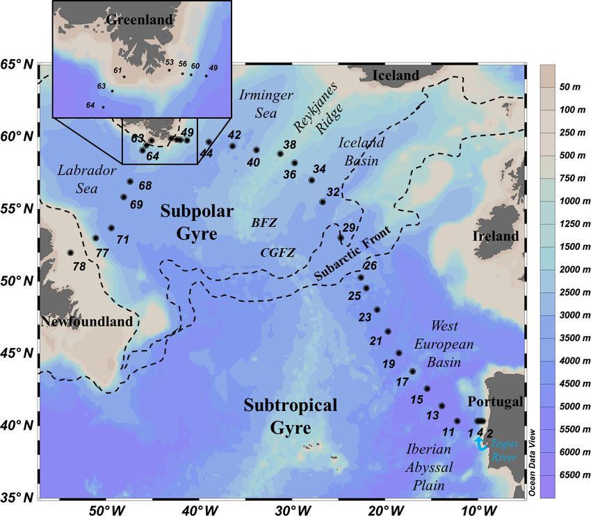
M. Tonnard et al.: Dissolved iron in the North Atlantic Ocean                                                                         919

Figure 1. Map of the GEOTRACES GA01 voyage plotted on bathymetry as well as the major topographical features and main basins (Ocean
Data View (ODV) software, version 4.7.6, Schlitzer, 2016; http://odv.awi.de, last access: 30 January 2020). BFZ: Bight Fracture Zone; CGFZ:
Charlie-Gibbs Fracture Zone.

2     Material and methods                                              surface waters, the shallowest sampling depth was 15 m at
                                                                        all stations. Therefore, “surface water samples” refers to
2.1    Study area and sampling activities                               15 m depth.
                                                                           Samples were collected using a trace metal clean
                                                                        polyurethane powder-coated aluminum frame rosette (here-
Samples were collected during the GEOVIDE
                                                                        after referred to as TMR) equipped with twenty-two 12 L,
(GEOTRACES-GA01 section, Fig. 1) oceanographic voy-
                                                                        externally closing, Teflon-lined GO-FLO bottles (General
age from 15 May 2014 (Lisbon, Portugal) to 30 June 2014
                                                                        Oceanics) and attached to a Kevlar® line. The cleaning proto-
(St. John’s, Newfoundland, Canada) aboard N/O Pourquoi
                                                                        cols for sampling bottles and equipment followed the guide-
Pas?. The study was carried out along the OVIDE line
                                                                        lines of the GEOTRACES Cookbook (http://www.geotraces.
(http://www.umr-lops.fr/Projets/Projets-actifs/OVIDE, last
                                                                        org, last access: 30 January 2020, Cutter et al., 2017). After
access: 30 January 2020, previously referred to as the
                                                                        TMR recovery, GO-FLO bottles were transferred into a clean
WOCE A25 Greenland-to-Portugal section) and in the
                                                                        container equipped with a class 100 laminar flow hood. Sam-
Labrador Sea (corresponding to the WOCE A01 leg 3
                                                                        ples were either taken from the filtrate of particulate sam-
Greenland-to-Newfoundland section). The OVIDE line has
                                                                        ples (collected on polyethersulfone filters, 0.45 µm supor® ;
been sampled every 2 years since 2002 in the North Atlantic
                                                                        see Gourain et al., 2019) or after filtration using 0.2 µm fil-
(e.g., Mercier et al., 2015) and in the Labrador Sea (broadly
                                                                        ter cartridges (Sartorius Sartobran® 300) due to water budget
corresponding to the WOCE A01 leg 3 Greenland-to-
                                                                        restriction (Table 1). Filtration techniques were not directly
Newfoundland section). In total, 32 stations were occupied,
                                                                        compared for the same samples; however, Wilcoxon statisti-
and samples were usually collected at 22 depths, except
                                                                        cal tests were performed to compare the distribution of DFe
at shallower stations close to the Iberian, Greenland, and
                                                                        at each pair of adjacent stations where the change of filtra-
Canadian shelves (Fig. 1) where fewer samples (between
                                                                        tion technique was performed (see Table 1). No significant
6 and 11) were collected. To avoid ship contamination of

www.biogeosciences.net/17/917/2020/                                                                Biogeosciences, 17, 917–943, 2020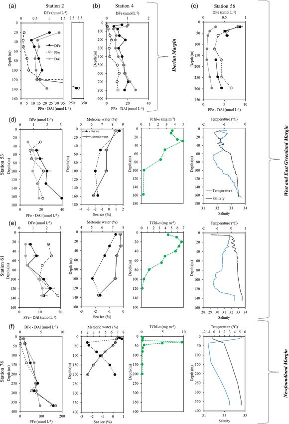
920                                                           M. Tonnard et al.: Dissolved iron in the North Atlantic Ocean

differences were observed (p value > 0.2) for all pairs of sta-   cleaned following the GEOTRACES protocol (Cutter et al.,
tions (n = 9), except between stations 11 and 13 and between      2017).
stations 13 and 15. Moreover, both filtration techniques are         Mixed-element standard solution was prepared gravimet-
deemed acceptable by the GEOTRACES guidelines. Seawa-             rically using high-purity standards (Fe, Mn, Cd, Co, Zn,
ter was collected in acid-cleaned 60 mL LDPE bottles, after       Cu, Pb; SCP Science calibration standards) in HNO3 3 %
rinsing three times with about 20 mL of seawater. Teflon®         (v/v) (Merck Ultrapur® ). The distribution of the trace metals
tubing used to connect the filter holders or cartridges to the    other than Fe will be reported elsewhere (Planquette et al.,
GO-FLO bottles was washed in an acid bath (10 % v/v HCl,          2020). A six-point calibration curve was prepared by stan-
Suprapur® , Merck) for at least 12 h and rinsed three times       dard additions of the mixed element standard to our acid-
with ultra-high-purity water (UHPW > 18 M cm) prior to           ified in-house standard and ran at the beginning, the mid-
use. Samples were then acidified to ∼ pH 1.7 with HCl             dle, and the end of each analytical session. Each analytical
(Ultrapur® Merck, 2 ‰ v/v) under a class 100 laminar flow         session consisted of about 50 samples. Final concentrations
hood inside the clean container. The sample bottles were then     of samples and procedural blanks were calculated from In-
double bagged and stored at ambient temperature in the dark       normalized data. Data were blank-corrected by subtracting
before shore-based analyses 1 year after collection.              an average acidified Milli-Q blank that was preconcentrated
   Large volumes of seawater sample (referred to hereafter        on the seaFAST-pico™ in the same way as the samples and
as the in-house standard seawater) were also collected us-        seawater standards. The errors associated with each sam-
ing a towed fish at around 2–3 m deep and filtered in-line        ple were calculated as the standard deviation for five mea-
inside a clean container through a 0.2 µm pore size filter cap-   surements of low-Fe seawater samples. The mean Milli-Q
sule (Sartorius SARTOBRAN® 300) and stored unacidified            blank was equal to 0.08 ± 0.09 nmol L−1 (n = 17) consider-
in 20–30 L LDPE carboys (Nalgene™). All the carboys were          ing all analytical sessions. The detection limit, calculated for
cleaned following the guidelines of the GEOTRACES Cook-           a given run as 3 times the standard deviation of the Milli-Q
book (Cutter et al., 2017). This in-house standard seawa-         blanks, was on average 0.05 ± 0.05 nmol L−1 (n = 17). Re-
ter was used for calibration on the seaFAST-pico™ SF-ICP-         producibility was assessed through the standard deviation of
MS (see Sect. 2.2) and was acidified to ∼ pH 1.7 with HCl         replicate samples (every 10th sample was a replicate) and
(Ultrapur® Merck, 2 ‰ v/v) at least 24 h prior to analysis.       the average of the in-house standard seawater and was equal
                                                                  to 17 % (n = 84). Accuracy was determined from the analy-
2.2   DFe analysis with seaFAST-pico™                             sis of consensus (SAFe S, GSP) and certified (NASS-7) sea-
                                                                  water matrices (see Table 2) and in-house standard seawater
Seawater samples were preconcentrated using a seaFAST-            (DFe = 0.42 ± 0.07 nmol L−1 , n = 84). Note that all the DFe
pico™ (ESI, Elemental Scientific, USA) and the eluent             values were generated in nanomoles per kilogram using the
was directly introduced via a perfluoroalkoxy alkane screw-       seaFAST-pico™ coupled to an Element XR SF-ICP-MS and
thread (PFA-ST) nebulizer and a cyclonic spray chamber in         were converted to nanomoles per liter using the actual den-
an Element XR sector field inductively coupled plasma mass        sity (kg L−1 ) of each seawater sample (Table 1) to be directly
spectrometer (Element XR SF-ICP-MS, Thermo Fisher Sci-            comparable with literature.
entific Inc., Omaha, NE), following the protocol of Lager-
ström et al. (2013).                                              2.3   Meteoric water and sea ice fraction calculation
   High-purity-grade solutions and water (Milli-Q) were
used to prepare the following reagents each day: the acetic       We considered the different contributions of sea ice melt
acid–ammonium acetate buffer (CH3 COO− and NH+                    (SIM), meteoric water (MW), and saline seawater, at Sta-
                                                      4 ) was
made of 140 mL acetic acid (>99 % NORMATOM® –                     tions 53, 61, and 78 using the procedure and mass balance
VWR Chemicals) and ammonium hydroxide (25 %, Merck                calculations that are fully described in Benetti et al. (2016).
Suprapur® ) in 500 mL PTFE bottles and was adjusted to            Briefly, we considered two types of seawater, namely At-
pH 6.0 ± 0.2 for the on-line pH adjustment of the sam-            lantic Water (AW) and Pacific Water (PW). The relative pro-
ples. The eluent was made of 1.4 M nitric acid (HNO3 ,            portions of AW (fAW ) and PW (fPW ) are calculated based on
Merck Ultrapur® ) in Milli-Q water by a 10-fold dilution and      the distinctive nitrogen-to-phosphorus (N–P) relationships
spiked with 1 µg L−1 115 In (SCP Science calibration stan-        for the two water masses (Jones et al., 1998) as follows (e.g.,
dards) to allow for drift correction. Autosampler and column      Sutherland et al., 2009):
rinsing solutions were made of HNO3 2.5 % (v/v) (Merck                    N m − N AW
Suprapur® ) in Milli-Q water. The carrier solution driven by      fPW =               ,                                       (1)
                                                                          N PW − N AW
the syringe pumps to move the sample and buffer through the
flow injection system was made in the same way.                   where N m is the measured dissolved inorganic nitrogen, and
   All reagents, standards, samples, and blanks were prepared     N AW and N PW are the values for pure Atlantic and Pa-
in acid-cleaned low-density polyethylene (LDPE) or Teflon         cific water, respectively, estimated from Jones et al. (1998),
fluorinated ethylene propylene (FEP) bottles. Bottles were        and N AW and N PW values are calculated by substituting the

Biogeosciences, 17, 917–943, 2020                                                       www.biogeosciences.net/17/917/2020/
M. Tonnard et al.: Dissolved iron in the North Atlantic Ocean                                                                            921

Table 1. Station number, date of sampling (in the dd/mm/yyyy format), pore size used for filtration (µm), station location, mixed-layer depth
(m), and associated average dissolved iron (DFe) concentrations, standard deviation, and number of samples during the GEOTRACES GA01
transect. Note that the asterisk next to station numbers refers to disturbed temperature and salinity profiles as opposed to uniform profiles.

                       Station      Date sampling   Filtration   Latitude    Longitude      Zm     DFe (nmol L−1 )
                                    (dd/mm/yyyy)         (µm)       (◦ N)        (◦ E)      (m)        average SD    n
                       1            19/05/2014            0.2      40.33           −10.04   25.8       1.07 ± 0.12   1
                       2            21/05/2014            0.2      40.33            −9.46   22.5       1.01 ± 0.04   1
                       4            21/05/2014            0.2      40.33            −9.77   24.2       0.73 ± 0.03   1
                       11           23/05/2014            0.2      40.33           −12.22   31.3       0.20 ± 0.11   2
                       13           24/05/2014           0.45      41.38           −13.89   18.8       0.23 ± 0.02   1
                       15           28/05/2014            0.2      42.58           −15.46   34.2       0.22 ± 0.03   2
                       17           29/05/2014            0.2      43.78           −17.03   36.2       0.17 ± 0.01   1
                       19∗          30/05/2014           0.45      45.05           −18.51   44.0       0.13 ± 0.05   2
                       21           31/05/2014            0.2      46.54           −19.67   47.4       0.23 ± 0.08   2
                       23∗          02/06/2014            0.2      48.04           −20.85   69.5       0.21 ± 0.05   6
                       25           03/06/2014            0.2      49.53           −22.02   34.3       0.17 ± 0.04   2
                       26           04/06/2014           0.45      50.28           −22.60   43.8       0.17 ± 0.03   2
                       29           06/06/2014           0.45      53.02           −24.75   23.8       0.17 ± 0.02   1
                       32           07/06/2014            0.2      55.51           −26.71   34.8       0.59 ± 0.08   2
                       34           09/06/2014           0.45      57.00           −27.88   25.6               NA    0
                       36           10/06/2014           0.45      58.21           −29.72   33.0       0.12 ± 0.02   1
                       38           10/06/2014           0.45      58.84           −31.27   34.5       0.36 ± 0.16   2
                       40           12/06/2014           0.45      59.10           −33.83   34.3       0.39 ± 0.05   1
                       42           12/06/2014           0.45      59.36           −36.40   29.6       0.36 ± 0.05   1
                       44           13/06/2014            0.2      59.62           −38.95   25.8               NA    0
                       49           15/06/2014           0.45      59.77           −41.30   60.3       0.30 ± 0.05   2
                       53∗          17/06/2014           0.45      59.90           −43.00   36.4               NA    0
                       56∗          17/06/2014           0.45      59.82           −42.40   30.0       0.87 ± 0.06   1
                       60∗          17/06/2014           0.45      59.80           −42.00   36.6       0.24 ± 0.02   2
                       61∗          19/06/2014           0.45      59.75           −45.11   39.8       0.79 ± 0.12   1
                       63∗          19/06/2014           0.45      59.43           −45.67   86.7       0.40 ± 0.03   1
                       64           20/06/2014           0.45      59.07           −46.09   33.9       0.27 ± 0.06   2
                       68∗          21/06/2014           0.45      56.91           −47.42   26.3       0.22 ± 0.01   1
                       69∗          22/06/2014           0.45      55.84           −48.09   17.5       0.24 ± 0.02   1
                       71           24/06/2014           0.45      53.69           −49.43   36.7       0.32 ± 0.04   2
                       77∗          26/06/2014           0.45      53.00           −51.10   26.1               NA    0
                       78           27/06/2014           0.45      51.99           −53.82   13.4       0.79 ± 0.05   1

                     NA: not available.

POm  4 value in the equation of the pure AW and PW N–P                      low:
lines from Jones et al. (1998). However, during GEOVIDE,
the phosphate-depleted near-surface values led to unrealis-                 fAW + fPW + fMW + fSIM = 1,                                   (2)
tic lower N PW than just below the subsurface. Therefore, for               fAW SAW + fPW SPW + fMW SMW + fSIM SSIM = Sm ,                (3)
all surface samples, the N PW was replaced by the values at
100 m. Then, the surface values were adjusted by a factor of                fAW δO18          18
                                                                                  AW + fPW δOPW + fMW δOMW
                                                                                                           18

dilution proportional to the sample salinity.                                        + fSIM δO18       18
                                                                                               SIM = δOm ,                                (4)
   After estimating fAW and fPW and their respective salin-
ity and δ 18 O affecting each sample, the contribution of SIM               where fAW , fPW , fMW , and fSIM are the relative fraction
and MW can be determined using measured salinity (Sm ) and                  of AW, PW, MW, and SIM. To calculate the relative frac-
δ 18 O (δO18
          m ). The mass balance calculations are presented be-              tions of AW, PW, MW, and SIM, we used the following
                                                                            end-members: SAW = 35, δO18  AW = +0.18 ‰ (Benetti et al.,
                                                                            2016); SPW = 32.5, δO18  PW = −1 ‰ (Cooper et al., 1997;
                                                                            Woodgate and Aagaard, 2005); SMW = 0, δO18MW = −18.4 ‰
                                                                            (Cooper et al., 2008); SSIM = 4, δO18
                                                                                                               SIM = +0.5 ‰ (Melling
                                                                            and Moore, 1995).

www.biogeosciences.net/17/917/2020/                                                                   Biogeosciences, 17, 917–943, 2020
922 M. Tonnard et al.: Dissolved iron in the North Atlantic Ocean
Table 2. SAFe S, GSP, and NASS-7 dissolved iron concentrations time was 2 h. The extracts were then analyzed by HPLC with
(DFe, nmol L-1) determined by the seaFAST-pico™ instruments a complete Agilent Technologies 1200 system (comprising
and their consensus (SAFe S, GSP; https://websites.pmc.ucsc.edu/ LC ChemStation software, a degasser, a binary pump, a re-
~kbruland/GeotracesSaFe/kwbGeotracesSaFe.html, last access: frigerated autosampler, a column thermostat, and a diode ar-
30 January 2020) and certified (NASS-7; https://www.nrc-cnrc.gc. ray detector) when possible on the same day as extraction.
ca/eng/solutions/advisory/crm/certificates/nass_7.html, last access:
The sample extracts were premixed (1 : 1) with a tetrabuty-
30 January 2020) DFe concentrations. Note that no consensual
value is reported for the GSP seawater.
lammonium acetate (TBAA) buffer solution (28 nM) prior to
injection in the HPLC. The mobile phase was a mix between
DFe values (nmol L−1 )
a solution (a) of TBAA 28 mM / methanol (30/70, v/v) and
a solution (b) of 100 % methanol (i.e., the organic solvent)
Sea FAST-pico™ Reference or certified with varying proportions during analysis. After elution, pig-
Seawater used Average (±SD) n Average (±SD) ment concentrations (mg m−3 ) were calculated according to
SAFe S 0.100 (±0.006) 2 0.095 (±0.008)
Beer–Lambert’s law (i.e., A = εLC) from the peak areas with
GSP 0.16 (±0.04) 15 0.155 (±0.05) an internal standard correction (vitamin E acetate, Sigma)
NASS-7 6.7 (±1.7) 12 6.3 (±0.5) and an external standard calibration (DHI Water and Envi-
ronment, Denmark). This method allowed the detection of
23 phytoplankton pigments. The detection limits, defined as
Negative sea ice fractions indicated a net brine release 3 times the signal : noise ratio for a filtered volume of 1 L,
while positive sea ice fractions indicated a net sea ice melt- was 0.0001 mg m−3 for total chlorophyll a (TChl a), and its
ing. Note that for stations over the Greenland Shelf, we as- injection precision was 0.91 %
sumed that the Pacific Water (PW) contribution was negli- All these data are available on the LEFE CYBER database
gible for the calculations, supported by the very low PW (http://www.obs-vlfr.fr/proof/php/geovide/geovide.php, last
fractions found at Cape Farewell in May 2014 (see Fig. B1 access: 30 January 2020).
in Benetti et al., 2017), while for station 78, located on the The mixed-layer depth (Zm ) for each station was calcu-
Newfoundland shelf, we used nutrient measurements to cal- lated using the function “calculate.mld” (part of the “rcal-
culate the PW fractions, following the approach from Jones cofi” package, Ed Weber at NOAA SWFSC) created by
et al. (1998) (the data are published in Benetti et al., 2017). Sam McClathie (NOAA Federal, 30 December 2013) for
R software and where Zm is defined as an absolute change
2.4 Ancillary measurements and mixed-layer depth in the density of seawater at a given temperature (1σθ ≥
determination 0.125 kg m−3 ) with respect to an approximately uniform re-
gion of density just below the ocean surface (Kara et al.,
Potential temperature (θ ), salinity (S), dissolved oxygen 2000). In addition to the density criterion, the temperature
(O2 ), and beam attenuation data were retrieved from and salinity profiles were inspected at each station for uni-
the conductivity–temperature–depth (CTD) sensors (CTD formity within this layer. When they were not uniform, the
SBE911 equipped with a SBE-43) that were deployed on a depth of any perturbation in the profile was chosen as the
stainless-steel rosette. Salinity profiles were calibrated using base of the Zm (Table 1).
1228 samples taken from the GO-FLO bottles, leading to a
precision of 0.002 psu. The O2 data could not be directly cal- 2.5 Statistical analysis
ibrated with GO-FLO samples, due to the sampling time be-
ing too long, so the calibrated O2 profiles acquired by the All statistical approaches, namely the comparison between
classic CTD at the same station were used to calibrate the the pore size used for filtration, correlations, and principal
O2 profiles of the TMR CTD, with a precision estimated at component analysis (PCA), were performed using the R sta-
3 µmol kg−1 . Nutrient and total chlorophyll a (TChl a) sam- tistical software (R development Core Team, 2012). For all
ples were collected using the classic CTD at the same sta- the results, p values were calculated against the threshold
tions as for the TMR. We used the data from the stainless- value alpha (α), which we assigned at 0.05, corresponding
steel rosette casts that were deployed immediately before or to a 95 % level of confidence. For all datasets, non-normal
after our TMR casts. Pigments were separated and quan- distributions were observed according to the Shapiro–Wilk
tified following an adaptation of the method described by test. Therefore, the significance level was determined with a
Van Heukelem and Thomas (2001) and the analytical pro- Wilcoxon test.
cedure used is described in Ras et al. (2008). The method All sections and surface layer plots were prepared using
adaptation allowed for higher sensitivity in the analysis of Ocean Data View (Schlitzer, 2016).
low-phytoplankton-biomass waters (see Ras et al., 2008).
Briefly, frozen filters were extracted at −20 ◦ C in 3 mL of
methanol (100 %), sonicated, and then clarified by vacuum
filtration through Whatman GF/F filters. The total extraction
Biogeosciences, 17, 917–943, 2020 www.biogeosciences.net/17/917/2020/M. Tonnard et al.: Dissolved iron in the North Atlantic Ocean 923 2.6 Water mass determination and associated DFe lar Mode Water (IcSPMW, 7.07
924                                                                   M. Tonnard et al.: Dissolved iron in the North Atlantic Ocean

Figure 2. Parameters measured from the regular CTD cast represented as a function of depth for the GA01 section for (a) dissolved oxygen
(O2 , µmol kg−1 ), (b) salinity, and (c) temperature (◦ C). The contour lines represent isopycnals (neutral density, γ n , in units of kilogram per
cubic meter) (Ocean Data View (ODV) software, version 4.7.6, Schlitzer, 2016; http://odv.awi.de, last access: 30 January 2020).

Biogeosciences, 17, 917–943, 2020                                                                    www.biogeosciences.net/17/917/2020/
M. Tonnard et al.: Dissolved iron in the North Atlantic Ocean                                                                925

to the bottom and is characterized by high silicic acid           ropean Basin exhibited enhanced NO−     3 concentrations as a
(42 ± 4 µmol L−1 ), nitrate (21.9 ± 1.5 µmol L−1 ) concentra-     result of mixing between ENACW and IcSPMW, although
tions and lower oxygen concentration (O2 ≈ 252 µmol kg−1 )        these surface waters were dominated by ENACW. In the
(see Sarthou et al., 2018). The core of the NEADW (sta-           Labrador Sea (stations 68–78) low surface concentrations
tions 1–13) was located near the seafloor and gradually de-       were observed with values ranging from 0.04 (station 68)
creased westward. Polar Intermediate Water (PIW, θ ≈ 0 ◦ C,       to 1.8 (station 71) µmol L−1 . At depth, the lowest concentra-
S ≈ 34.65) is a ventilated, dense, low-salinity water intrusion   tions (lower than 15.9 µmol L−1 ) were measured in ENACW
to the deep overflows within the Irminger and Labrador seas       (∼ 0–800 m depth) and DSOW (> 1400 m depth), while the
that is formed at the Greenland shelf. PIW represents only a      highest concentrations were measured within NEADW (up
small contribution to the whole water mass pool (up to 27 %)      to 23.5 µmol L−1 ) and in the mesopelagic zone of the West
and was observed over the Greenland slope at stations 53          European and Iceland basins (higher than 18.4 µmol L−1 ).
and 61 as well as in surface waters from station 63 (from
0 to ∼ 200 m depth), in intermediate waters of stations 49,       3.2.2    Chlorophyll a
60, and 63 (from ∼ 500 to ∼ 1500 m depth) and in bottom
waters of stations 44, 68, 69, 71, and 77 with a contribution     Overall, most of the phytoplankton biomass was localized
higher than 10 %. Iceland–Scotland Overflow Water (ISOW,          above 100 m depth with lower total chlorophyll a (TChl a)
θ ≈ 2.6 ◦ C, S ≈ 34.98) is partly formed within the Arctic        concentrations south of the Subarctic Front and higher at
Ocean by convection of the modified Atlantic water. ISOW          higher latitudes (see Supplement Fig. S1). While compar-
comes from the Iceland–Scotland sills and flows southward         ing TChl a maxima considering all stations, the lowest
towards the Charlie-Gibbs Fracture Zone (CGFZ) and Bight          value (0.35 mg m−3 ) was measured within the West Euro-
Fracture Zone (BFZ) (stations 34 and 36), after which it re-      pean Basin (station 19, 50 m depth) while the highest val-
verses its flowing path northward and enters the Irminger Sea     ues were measured at the Greenland (up to 4.9 mg m−3 , 30 m
(stations 40 and 42) to finally reach the Labrador Sea close      depth, station 53, and up to 6.6 mg m−3 , 23 m depth, station
to the Greenland coast (station 49, station 44 being located      61) and Newfoundland (up to 9.6 mg m−3 , 30 m depth, sta-
in between these two opposite flow paths). Along the eastern      tion 78) margins.
(stations 26–36) and western (stations 40–44) flanks of the
Reykjanes Ridge, ISOW had a contribution higher than 50 %         3.3     Dissolved Fe concentrations
to the water mass pool. ISOW was observed from 1500 m
depth to the bottom of the entire Iceland Basin (stations 29–     Dissolved Fe concentrations (see Supplement Table S1)
38) and from 1800 to 3000 m depth within the Irminger Sea         ranged from 0.09 ± 0.01 nmol L−1 (station 19, 20 m depth)
(stations 40–60). ISOW, despite having a fraction lower than      to 7.8 ± 0.5 nmol L−1 (station 78, 371 m depth) (see Fig. 3).
45 % above the Reykjanes Ridge (station 38), was the main         Generally, vertical profiles of DFe for stations above the mar-
contributor to the water mass pool from 1300 m depth down         gins (2, 4, 53, 56, 61, and 78) showed an increase with depth,
to the bottom. ISOW was also observed within the Labrador         although sea-surface maxima were observed at stations 2, 4,
Sea from stations 68 to 77. Finally, the deepest part of the      and 56. For these margin stations, values ranged from 0.7
Irminger (stations 42 and 44) and Labrador (stations 68–          to 1.0 nmol L−1 in the surface waters. Concentrations in-
71) seas was occupied by Denmark Strait Overflow Water            creased towards the bottom, with more than 7.8 nmol L−1
(DSOW, θ ≈ 1.30 ◦ C, S ≈ 34.905).                                 measured at station 78; approximately 1–3 nmol L−1 for sta-
                                                                  tions 2, 4, 53, and 61; and just above 0.4 nmol L−1 for station
3.2     Ancillary data                                            56 (Fig. 4). Considering the four oceanic basins, mean verti-
                                                                  cal profiles (Fig. S2) showed increasing DFe concentrations
3.2.1    Nitrate                                                  down to 3000 m depth followed by decreasing DFe concen-
                                                                  trations down to the bottom. Among deep-water masses, the
Surface nitrate (NO− 3 ) concentrations (García-Ibáñez et al.,    lowest DFe concentrations were measured in the West Euro-
2018; Pérez et al., 2018; Sarthou et al., 2018) ranged from       pean Basin. The Irminger Sea displayed the highest DFe con-
0.01 to 10.1 µmol L−1 (stations 53 and 63, respectively).         centrations from 1000 m depth to the bottom relative to other
There was considerable spatial variability in NO−   3 surface     basins at similar depths (Figs. 3 and S2). In the Labrador
distributions with high concentrations found in the Iceland       Sea, DFe concentrations were low and relatively constant
Basin and Irminger Sea (higher than 6 µmol L−1 ), as well         at about 0.87 ± 0.06 nmol L−1 from 250 to 3000 m depth
as at stations 63 (10.1 µmol L−1 ) and 64 (5.1 µmol L−1 ), and    (Fig. S2). Overall, surface DFe concentrations were higher
low concentrations observed in the West European Basin, in        (0.36 ± 0.18 nmol L−1 ) in the North Atlantic Subpolar Gyre
the Labrador Sea, and above continental margins. The low          (above 52◦ N) than in the North Atlantic subtropical gyre
surface concentrations in the West European Basin ranged          (0.17±0.05 nmol L−1 ). The surface DFe concentrations were
from 0.02 (station 11) to 3.9 (station 25) µmol L−1 . Station     generally smaller than 0.3 nmol L−1 , except for a few stations
26 delineating the extreme western boundary of the West Eu-       in the Iceland Basin (stations 32 and 38) and Irminger (sta-

www.biogeosciences.net/17/917/2020/                                                        Biogeosciences, 17, 917–943, 2020
926 M. Tonnard et al.: Dissolved iron in the North Atlantic Ocean
tions 40 and 42) and Labrador (station 63) seas, where values 4 Discussion
ranged between 0.4 and 0.5 nmol L−1 .
In the following sections, we will first discuss the high DFe
3.4 DFe signatures in water masses concentrations observed throughout the water column of sta-
tions 1 and 17 located in the West European Basin (Sect. 4.1)
In the Labrador Sea, IrSPMW exhibited an average DFe con- and then the relationship between water masses and the DFe
centration of 0.61 ± 0.21 nmol L−1 (n = 14). DFe concentra- concentrations (Sect. 4.2) in intermediate (Sect. 4.2.2 and
tions in the LSW were the lowest in this basin, with an av- 4.2.3) and deep (Sect. 4.2.4 and 4.2.5) waters. We will also
erage value of 0.71 ± 0.27 nmol L−1 (n = 53) (see Fig. S3). discuss the role of wind (Sect. 4.2.1), rivers (Sect. 4.3.1), me-
Deeper, ISOW displayed slightly higher average DFe con- teoric water and sea ice processes (Sect. 4.3.2), atmospheric
centrations (0.82 ± 0.05 nmol L−1 , n = 2). Finally, DSOW deposition (Sect. 4.3.3), and sediments (Sect. 4.4) in deliver-
had the lowest average (0.68 ± 0.06 nmol L−1 , n = 3; see ing DFe. Finally, we will discuss the potential Fe limitation
Fig. S3) and median (0.65 nmol L−1 ) DFe values for inter- using DFe : NO− 3 ratios (Sect. 4.5).
mediate and deep waters.
In the Irminger Sea, surface waters were composed of 4.1 High DFe concentrations at stations 1 and 17
SAIW (0.56 ± 0.24 nmol L−1 , n = 4) and IrSPMW (0.72 ±
0.32 nmol L−1 , n = 34). The highest open-ocean DFe con- Considering the entire section, two stations (stations
centrations (up to 2.5 ± 0.3 nmol L−1 , station 44, 2600 m 1 and 17) showed irregularly high DFe concentrations
depth) were measured within this basin. In the upper in- (> 1 nmol L−1 ) throughout the water column, thus suggest-
termediate waters, LSW was identified only at stations 40 ing analytical issues. However, these two stations were ana-
to 44 and had the highest DFe values with an average of lyzed twice and provided similar results, therefore discarding
1.2±0.3 nmol L−1 (n = 14). ISOW showed higher DFe con- any analytical issues. This means that these high values orig-
centrations than in the Iceland Basin (1.3 ± 0.2 nmol L−1 , inated either from genuine processes or from contamination
n = 4). At the bottom, DSOW was mainly located at sta- issues. If there had been contamination issues, one would ex-
tions 42 and 44 and presented the highest average DFe values pect a more random distribution of DFe concentrations and
(1.4 ± 0.4 nmol L−1 , n = 5) as well as the highest variabil- less consistence throughout the water column. It thus appears
ity from all the water masses presented in this section (see that contamination issues were unlikely to happen. Similarly,
Fig. S3). the influence of water masses to explain these distributions
In the Iceland Basin, SAIW and IcSPMW displayed simi- was discarded as the observed high homogenized DFe con-
lar averaged DFe concentrations (0.67 ± 0.30 nmol L−1 , n = centrations were restricted to these two stations. Station 1,
7 and 0.55 ± 0.34 nmol L−1 , n = 22, respectively). Averaged located at the continental shelf break of the Iberian Margin,
DFe concentrations were similar in both LSW and ISOW and also showed enhanced PFe concentrations from lithogenic
higher than in SAIW and IcSPMW (0.96 ± 0.22 nmol L−1 , origin suggesting a margin source (Gourain et al., 2019).
n = 21 and 1.0 ± 0.3 nmol L−1 , n = 10, respectively; see Conversely, no relationship was observed between DFe and
Fig. S3). PFe nor transmissometry for station 17. However, Ferron et
Finally, in the West European Basin, DFe concentrations al. (2016) reported a strong dissipation rate at the Azores-
in ENACW were the lowest of the whole section with an Biscay Rise (station 17) due to internal waves. The associ-
average value of 0.30 ± 0.16 nmol L−1 (n = 64). MOW was ated vertical energy fluxes could explain the homogenized
present deeper in the water column but was not character- profile of DFe at station 17, although such waves are not
ized by particularly high or low DFe concentrations relative clearly evidenced in the velocity profiles. Consequently, the
to the surrounding Atlantic waters (see Fig. S3). The median elevated DFe concentrations observed at station 17 remain
DFe value in MOW was very similar to the median value unsolved.
when considering all water masses (0.75 and 0.77 nmol L−1 ,
respectively, Fig. S3). LSW and IcSPMW displayed slightly 4.2 DFe and hydrology key points
elevated DFe concentrations compared to the overall median
4.2.1 How do air–sea interactions affect DFe
with mean values of 0.82 ± 0.08 (n = 28) and 0.80 ± 0.04
concentration in the Irminger Sea?
(n = 8) nmol L−1 , respectively. The DFe concentrations in
NEADW were relatively similar to the DFe median value of Among the four distinct basins described in this paper,
the GEOVIDE voyage (0.71 and 0.77 nmol L−1 , respectively, the Irminger Sea exhibited the highest DFe concentrations
Fig. S3). within the surface waters (from 0 to 250 m depth) with values
ranging from 0.23 to 1.3 nmol L−1 for open-ocean stations.
Conversely, low DFe concentrations were previously re-
ported in the central Irminger Sea by Rijkenberg et al. (2014)
(April–May, 2010) and Achterberg et al. (2018) (April–May
and July–August, 2010) with DFe concentrations ranging
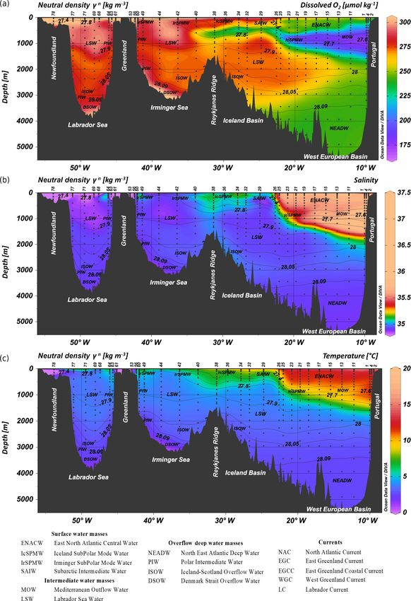
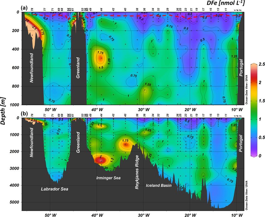
Biogeosciences, 17, 917–943, 2020 www.biogeosciences.net/17/917/2020/M. Tonnard et al.: Dissolved iron in the North Atlantic Ocean 927 Figure 3. Contour plot of the distribution of dissolved iron (DFe) concentrations in nanomoles per liter along the GA01 voyage transect: upper 1000 m (a) and full depth range (b). The red dashed line indicates the depth of the surface mixed layer (SML). Small black dots represent collected water samples at each sampling station (Ocean Data View (ODV) software, version 4.7.6; Schlitzer, 2016; http://odv.awi.de). from 0.11 to 0.15 and from ∼ 0 to 0.14 nmol L−1 , respec- ocean (de Jong et al., 2012; Louanchi and Najjar, 2001). tively (see Fig. S4 and Table S2). Differences might be due Deep convective winter mixing is triggered by the effect to the phytoplankton bloom advancement, the high reminer- of wind and a preconditioning of the ocean in such a way alization rate (Lemaitre et al., 2018b) observed within the that the inherent stability of the ocean is minimal. Pickart LSW in the Irminger Sea (see Sect. 4.1.3), and a deeper win- et al. (2003) demonstrated that these conditions are satisfied ter convection in early 2014. Indeed, enhanced surface DFe in the Irminger Sea with the presence of weakly stratified concentrations measured during GEOVIDE in the Irminger surface water, a close cyclonic circulation, which leads to Sea could be due to intense wind forcing events that would the shoaling of the thermocline, and intense winter air–sea deepen the winter Zm down to the core of the Fe-rich LSW. buoyancy fluxes (Marshall and Schott, 1999). Moore (2003) In the North Atlantic Ocean, the warm and salty water and Piron et al. (2016) described low-altitude westerly jets masses of the upper limb of the AMOC are progressively centered northeast of Cape Farewell, over the Irminger Sea, cooled and become denser, and they subduct into the abyssal known as tip jet events. These events occur when wind is ocean. In some areas of the subpolar North Atlantic, deep split around the orographic features of Cape Farewell and convective winter mixing provides a rare connection between are strong enough to induce deep convective mixing (Bacon surface and deep waters of the AMOC, thus constituting an et al., 2003; Pickart et al., 2003). It has also been shown important mechanism in supplying nutrients to the surface that during winters with a positive North Atlantic Oscilla- www.biogeosciences.net/17/917/2020/ Biogeosciences, 17, 917–943, 2020
928                                                                   M. Tonnard et al.: Dissolved iron in the North Atlantic Ocean

Figure 4. Vertical profiles of dissolved iron (DFe, black dots, solid line), particulate iron (PFe, black open dots, dashed line; Gourain et al.,
2019), and dissolved aluminum (DAl, grey dots; Menzel Barraqueta et al., 2018) at stations 2 (a), and 4 (b) located above the Iberian shelf;
station 56 (c), station (d) 53 and station 61 (e) located above the Greenland shelf; and station 78 (f) located above the Newfoundland shelf.
Note that for stations 53, 61, and 78, plots of the percentage of meteoric water (open dots) and sea ice melting (black dots and dashed line)
(Benetti et al., 2017, see text for details), total chlorophyll a (TChl a, green), temperature (blue), and salinity (black) are also displayed as a
function of depth.

Biogeosciences, 17, 917–943, 2020                                                                    www.biogeosciences.net/17/917/2020/
M. Tonnard et al.: Dissolved iron in the North Atlantic Ocean                                                               929

tion (NAO) index, the occurrence of such events is favored        MOW signal from the remineralization signal (Sarthou et al.,
(Moore, 2003; Pickart et al., 2003), which was the case in        2007). On the other hand, differences between studies likely
the winter of 2013–2014, preceding the GEOVIDE voyage             originate from the intensity of atmospheric deposition and
as opposed to previous studies (Pascale Lherminier, personal      the nature of aerosols. Indeed, Wagener et al. (2010) high-
communication, 2019). The winter mixed-layer depth prior          lighted that large dust deposition events can accelerate the
to the cruise reached up to 1200 m depth in the Irminger Sea      export of Fe from the water column through scavenging. As
(Zunino et al., 2017), which was most likely attributed to a      a result, in seawater with high DFe concentrations and where
final deepening due to wind forcing events (centered at sta-      high dust deposition occurs, a strong individual dust deposi-
tion 44). Such winter entrainment was likely the process in-      tion event could act as a sink for DFe. It thus becomes less
volved in the vertical supply of DFe within surface waters fu-    evident to observe a systematic high-DFe signature in MOW
eling the spring phytoplankton bloom with DFe values close        despite dust inputs.
to those found in LSW.
                                                                  4.2.3   Fe enrichment in Labrador Sea Water (LSW)
4.2.2   Why do we not see a DFe signature in the
        Mediterranean Overflow Water (MOW)?
                                                                  As described in Sect. 3.1, the LSW exhibited increasing DFe
On its northern shores, the Mediterranean Sea is bordered         concentrations from its source area, the Labrador Sea, to-
by industrialized European countries, which act as a contin-      ward the other basins, with the highest DFe concentrations
uous source of anthropogenically derived constituents into        observed within the Irminger Sea, suggesting that the wa-
the atmosphere, and on the southern shores by the arid and        ter mass was enriched in DFe either locally in each basin or
desert regions of the north African and Arabian Desert belts,     during its flow path (see Fig. S3). These DFe sources could
which act as sources of crustal material in the form of dust      originate from a combination of high export of PFe and its
pulses (Chester et al., 1993; Guerzoni et al., 1999; Martin       remineralization in the mesopelagic area and/or the dissolu-
et al., 1989). During the summer, when thermal stratification     tion of sediment.
occurs, DFe concentrations in the SML can increase over the          The Irminger and Labrador seas exhibited the highest av-
whole Mediterranean Sea by 1.6–5.3 nmol L−1 in response to        eraged integrated TChl-a concentrations (98 ± 32 and 59 ±
the accumulation of atmospheric Fe from both anthropogenic        42 mg m−2 ) compared to the West European and Iceland
and natural origins (Bonnet and Guieu, 2004; Guieu et al.,        basins (39 ± 10 and 53 ± 16 mg m−2 ), when the influence of
2010; Sarthou and Jeandel, 2001). After atmospheric deposi-       margins was discarded. Stations located in the Irminger (sta-
tion, the fate of Fe will depend on the nature of aerosols, Fe–   tions 40–56) and Labrador (stations 63–77) seas were largely
ligand binding capacity, vertical mixing, biological uptake,      dominated by diatoms (> 50 % of phytoplankton abundances)
and scavenging processes (Bonnet and Guieu, 2006; Wuttig          and displayed the highest chlorophyllide a concentrations,
et al., 2013). During GEOVIDE, MOW was observed at per-           a tracer of senescent diatom cells, likely reflecting post-
centages higher than ∼ 60 % from stations 1 to 13 between         bloom conditions (Tonnard et al., in prep.). This is in line
900 and 1100 m depth and associated with high dissolved           with the highest POC export data reported by Lemaitre et
aluminum (DAl; Menzel Barraqueta et al., 2018) concentra-         al. (2018a) in these two oceanic basins. This likely suggests
tions (up to 38.7 nmol L−1 ), confirming the high atmospheric     that biogenic PFe export was also higher in the Labrador
deposition in the Mediterranean region. In contrast to Al, no     and Irminger seas than in the West European and Ice-
DFe signature was associated with MOW (Figs. 2 and 3). Us-        land basins. In addition, Gourain et al. (2019) highlighted
ing LADCP data during the cruise, we estimated a translation      a higher biogenic contribution for particles located in the
velocity for the MOW of ∼ 3–8 cm s−1 , consistent with pre-       Irminger and Labrador seas with relatively high PFe : PAl
vious published values (e.g., Armi et al., 1989; Schmidt et       ratios (0.44 ± 0.12 mol : mol and 0.38 ± 0.10 mol : mol, re-
al., 1996). Our station 13 was located ∼ 2000 km away from        spectively) compared to particles from the West European
the origin of the MOW, which would mean a transit time of         and Iceland basins (0.22 ± 0.10 and 0.38 ± 0.14 mol : mol,
∼ 1–2 years. This transit time would allow the Fe signal to       respectively; see Fig. 6a in Gourain et al., 2019). How-
be preserved, when DFe residence times range from weeks           ever, they reported no difference in PFe concentrations be-
to months in the surface waters and from tens to hundreds of      tween the four oceanic basins, when the influence of mar-
years in deep waters (de Baar and de Jong, 2001; Sarthou et       gins was discarded, which likely highlighted the remineral-
al., 2003; Croot et al., 2004; Bergquist and Boyle 2006; Ger-     ization of PFe within the Irminger and Labrador seas. Indeed,
ringa et al., 2015; Tagliabue et al., 2016). This feature was     Lemaitre et al. (2018b) reported higher remineralization rates
also reported in some studies (Hatta et al., 2015; Thuróczy       within the Labrador (up to 13 mmol C m−2 d−1 ) and Irminger
et al., 2010), while others measured higher DFe concentra-        seas (up to 10 mmol C m−2 d−1 ) using the excess barium
tions in MOW (Gerringa et al., 2017; Sarthou et al., 2007).       proxy (Dehairs et al., 1997), compared to the West European
However, MOW coincides with the maximum apparent oxy-             and Iceland basins (ranging from 4 to 6 mmol C m−2 d−1 ).
gen utilization (AOU) and it is not possible to distinguish the   Therefore, the intense remineralization rates measured in the

www.biogeosciences.net/17/917/2020/                                                        Biogeosciences, 17, 917–943, 2020
930 M. Tonnard et al.: Dissolved iron in the North Atlantic Ocean
Irminger and Labrador seas likely resulted in enhanced DFe and Table S1), it appeared to be unlikely that these high DFe
concentrations within LSW. concentrations are the result of local sediment inputs, as no
Higher DFe concentrations were, however, measured in DFe gradient from the deepest samples to those above was
the Irminger Sea compared to the Labrador Sea and co- observed.
incided with lower transmissometry values (i.e., 98.0 %– Looking at salinity versus depth for these three stations,
98.5 % vs. > 99 %), thus suggesting a particle load of the one can observe the intrusion of Polar Intermediate Water
LSW. This could be explained by the reductive dissolution (PIW) at station 44 during GEOVIDE, which was not ob-
of Newfoundland Margin sediments. Indeed, Lambelet et served during the GA02 voyage and which contributed to
al. (2016) reported high dissolved neodymium (Nd) concen- about 14 % of the water mass composition (García-Ibáñez
trations (up to 18.5 pmol kg−1 ) within the LSW at the edge et al., 2018) and might therefore be responsible for the
of the Newfoundland Margin (51.82◦ N, 45.73◦ W) as well high DFe concentrations (see Fig. S5a). On the other hand,
as slightly lower Nd isotopic ratio values relative to those the PIW was also observed at stations 49 (from 390 to
observed in the Irminger Sea. They suggested that this wa- 1240 m depth), 60 (from 440 to 1290 m depth), 63 (from
ter mass had been in contact with sediments approximately 20 to 1540 m depth), 68 (3340 m depth), 69 (from 3200 to
within the last 30 years (Charette et al., 2015). Similarly, dur- 3440 m depth), 71 (from 2950 to 3440 m depth), and 77
ing GA03, Hatta et al. (2015) attributed the high DFe concen- (60 and 2500 m depth) with similar or higher contributions
trations in the LSW to continental margin sediments. Conse- of the PIW without such high DFe concentrations (maxi-
quently, it is also possible that the elevated DFe concentra- mum DFe = 1.3±0.1 nmol L−1 , 1240 m depth at station 49).
tions from the three LSW branches which entered the West At this station, the DSOW relative abundance was more
European and Iceland basins and Irminger Sea were supplied than 20 % (Fig. S5). The overflow of this dense water in
through sediment dissolution (Measures et al., 2013) along the Irminger Sea is associated with intense cyclonic boluses
the LSW pathway. (Käse et al., 2003) and the entrainment of waters from the
The enhanced DFe concentrations measured in the Greenland margin and slope by pulses of DSOW occurs all
Irminger Sea and within the LSW were thus likely attributed along its transport from Denmark Strait to the Greenland tip
to the combination of higher productivity, POC export, and (Magaldi et al., 2011; von Appen et al., 2014). This phe-
remineralization as well as a DFe supply from reductive nomenon may enrich the DSOW with Fe as well as other
dissolution of Newfoundland sediments to the LSW along elements. This was also observed for radium and actinium
its flow path. Using temperature and salinity anomalies, with a deviation from the conservative behavior of 226 Ra (Le
Yashayaev et al. (2007) showed that the LSW reached the Roy et al., 2018) and an increase in 227 Ac activity at station
Irminger Sea and the Iceland Basin in 1–2 and 4–5 years, re- 44 at 2500 m, reflecting inputs of these tracers. Therefore, the
spectively, after its formation in the Labrador Sea. The LSW high DFe concentrations observed in the Irminger Sea might
transit time in this region is thus compatible with DFe resi- be inferred from a substantial load of Fe-rich particles when
dence times (see above). DSOW is in contact with the Greenland margin.
4.2.4 Enhanced DFe concentrations in the Irminger 4.2.5 Reykjanes Ridge: hydrothermal inputs or Fe-rich
Sea bottom water seawater?
Bottom waters from the Irminger Sea exhibited the highest Hydrothermal activity was assessed over the Mid-Atlantic
DFe concentrations from the whole section, excluding the Ridge, namely the Reykjanes Ridge (RR), from stations 36
stations at the margins. Such a feature could be due to (i) ver- to 40. Indeed, within the inter-ridge database (http://www.
tical diffusion from local sediment, (ii) lateral advection of interridge.org, last access: 30 January 2020), the Reykjanes
water mass(es) displaying enhanced DFe concentrations, and Ridge is reported to have active hydrothermal sites. The sites
(iii) local dissolution of Fe from particles. Hereafter, we dis- were either confirmed (Baker and German, 2004; German et
cuss the plausibility of these three hypotheses. al., 1994; Olaffson et al., 1991; Palmer et al., 1995) close to
The GEOTRACES GA02 voyage (leg 1, 64PE319) which Iceland or inferred (e.g., Chen, 2003; Crane et al., 1997; Ger-
occurred in April–May 2010 from Iceland to Bermuda man et al., 1994; Sinha et al., 1997; Smallwood and White,
sampled two stations north and south of our station 44 1998) closer to the GEOVIDE section as no plume was de-
(59.62◦ N, ∼ 38.95◦ W): station 5 (60.43◦ N, ∼ 37.91◦ W) tected but a high backscatter was reported, potentially cor-
and 6 (58.60◦ N, ∼ 39.71◦ W), respectively. High DFe con- responding to a lava flow. Therefore, hydrothermal activ-
centrations in samples collected close to the bottom were ity at the sampling sites remains unclear with no elevated
also observed and attributed to sediment inputs highlighting DFe concentrations nor temperature anomaly above the ridge
boundary exchange between seawater and surface sediment (station 38). However, enhanced DFe concentrations (up to
(Lambelet et al., 2016; Rijkenberg et al., 2014). However, 1.5 ± 0.22 nmol L−1 , station 36, 2200 m depth) were mea-
because a decrease in DFe concentrations was observed at sured east of the Reykjanes Ridge (Fig. 3). This could be
our station 44 from 2500 m depth down to the bottom (Fig. 3 due to hydrothermal activity and resuspension of sunken par-
Biogeosciences, 17, 917–943, 2020 www.biogeosciences.net/17/917/2020/M. Tonnard et al.: Dissolved iron in the North Atlantic Ocean 931
ticles at sites located north of the section and transported
through ISOW towards the section (Fig. 3). Indeed, Achter-
berg et al. (2018) highlighted at ∼ 60◦ N and over the Reyk-
janes Ridge a southward lateral transport of a Fe plume of up
to 250–300 km. In agreement with these observations, previ-
ous studies (e.g., Fagel et al., 1996, 2001; Lackschewitz et
al., 1996; Parra et al., 1985) reported marine sediment min-
eral clays in the Iceland Basin largely dominated by smectite
(> 60 %), a tracer of hydrothermal alteration of basaltic vol-
canic materials (Fagel et al., 2001; Tréguer and De La Rocha,
2013). Kanzow and Zenk (2014) investigated the fluctuations
of the ISOW plume around RR. The transit time, west of
RR, between 60◦ N and the Bight Fracture Zone (BFZ), was
around 5 months, compatible with the residence time of DFe
(see above). Hence, the high DFe concentrations measured
east of RR could be due to a hydrothermal source and/or the
resuspension of (basaltic) particles and their subsequent dis-
solution.
West of the Reykjanes Ridge, a DFe enrichment was also Figure 5. Plot of dissolved iron (DFe, filled circles) and dissolved
aluminum (DAl, open circles; Menzel Barraqueta et al., 2018) at
observed in ISOW at station 40 within the Irminger Sea
∼ 20 m, along the salinity gradient between stations 1, 2, 4, and
(Fig. 3). The low transmissometer values within ISOW in the
11 with linear regression equations. The numbers close to sample
Irminger Sea (station 44) compared to the Iceland Basin (sta- points represent the station numbers.
tion 32) suggested a higher particle load (Fig. 4a in Gourain
et al., 2019). These particles could come from the Bight Frac-
ture Zone (BFZ, 56.91◦ N and 32.74◦ W) (Fig. 1) (Lacksche- tic Doppler current profiler (SADCP) data revealed a north-
witz et al., 1996; Zou et al., 2017) since the transit time of the ward circulation with a velocity of around 0.1 m s−1 (Pas-
ISOW between BFZ and our station 40 is around 3 months cale Lherminier, Patricia Zunino, personal communication,
(Kanzow and Zenk, 2014). 2019). The transit time from the estuary to our stations above
the shelf is around 15 d (150 km), which is short enough
4.3 What are the main sources of DFe in surface to preserve the DFe signal. Our SML DFe inventories were
waters? about 3 times higher at station 1 (∼ 1 nmol L−1 ) than those
calculated during the GA03 voyage (∼ 0.3 nmol L−1 , sta-
During GEOVIDE, enhanced DFe surface concentrations tion 1). Atmospheric deposition was about 1 order of mag-
were observed at several stations (stations 1–4, 53, 61, 78) nitude higher during GA03 than during GA01 (Shelley et al.,
highlighting an external source of Fe to surface waters. The 2015, 2018); thus the atmospheric source seemed to be mi-
main sources able to deliver DFe to surface waters are river- nor during GA01. Consequently, the Tagus River appears as
ine inputs, glacial inputs, and atmospheric deposition. In the the most likely source responsible for these enhanced DFe
following sections, these potential sources of DFe to surface concentrations, either directly as input of DFe or indirectly
waters will be discussed. through Fe-rich sediment carried by the Tagus River and its
subsequent dissolution. The Tagus estuary is the largest in
4.3.1 Tagus riverine inputs the western European coast and very industrialized (Canário
et al., 2003; de Barros, 1986; Figueres et al., 1985; Gauden-
Enhanced DFe surface concentrations (up to 1.07 ± cio et al., 1991; Mil-Homens et al., 2009); it extends through
0.12 nmol L−1 ) were measured over the Iberian Margin (sta- an area of 320 km2 and is characterized by a large water flow
tions 1–4) and coincided with salinity minima (∼You can also read