Attribution of the Australian bushfire risk to anthropogenic climate change
←
→
Page content transcription
If your browser does not render page correctly, please read the page content below
Nat. Hazards Earth Syst. Sci., 21, 941–960, 2021
https://doi.org/10.5194/nhess-21-941-2021
© Author(s) 2021. This work is distributed under
the Creative Commons Attribution 4.0 License.

Attribution of the Australian bushfire
risk to anthropogenic climate change
Geert Jan van Oldenborgh1 , Folmer Krikken1 , Sophie Lewis2 , Nicholas J. Leach3 , Flavio Lehner4,5,6 ,
Kate R. Saunders7 , Michiel van Weele1 , Karsten Haustein8 , Sihan Li8,9 , David Wallom9 , Sarah Sparrow9 ,
Julie Arrighi10,11 , Roop K. Singh10 , Maarten K. van Aalst10,12,13 , Sjoukje Y. Philip1 , Robert Vautard14 , and
Friederike E. L. Otto8
1 Royal  Netherlands Meteorological Institute (KNMI), De Bilt, the Netherlands
2 School  of Science, University of New South Wales, Canberra, ACT, Australia
3 Atmospheric, Oceanic and Planetary Physics, Department of Physics, University of Oxford, Oxford, UK
4 Department of Earth and Atmospheric Sciences, Cornell University, Ithaca, USA
5 Climate and Global Dynamics Laboratory, National Center for Atmospheric Research, Boulder, USA
6 Institute for Atmospheric and Climate Science, ETH Zürich, Zurich, Switzerland
7 Delft Institute of Applied Mathematics, Delft University of Technology, Delft, the Netherlands
8 Environmental Change Institute, University of Oxford, Oxford, UK
9 Oxford e-Research Centre, University of Oxford, Oxford, UK
10 Red Cross Red Crescent Climate Centre, the Hague, the Netherlands
11 Global Disaster Preparedness Center, Washington, DC, USA
12 Faculty of Geo-Information Science and Earth Observation, University of Twente, Enschede, the Netherlands
13 International Research Institute for Climate and Society, Columbia University, New York, USA
14 Institut Pierre-Simon Laplace, Gif-sur-Yvette, France

Correspondence: Geert Jan van Oldenborgh (oldenborgh@knmi.nl)

Received: 3 March 2020 – Discussion started: 11 March 2020
Revised: 30 January 2021 – Accepted: 1 February 2021 – Published: 11 March 2021

Abstract. Disastrous bushfires during the last months             have become more likely by at least a factor of 2 due to the
of 2019 and January 2020 affected Australia, raising the          long-term warming trend. However, current climate models
question to what extent the risk of these fires was exacer-       overestimate variability and tend to underestimate the long-
bated by anthropogenic climate change. To answer the ques-        term trend in these extremes, so the true change in the like-
tion for southeastern Australia, where fires were particularly    lihood of extreme heat could be larger, suggesting that the
severe, affecting people and ecosystems, we use a physically      attribution of the increased fire weather risk is a conserva-
based index of fire weather, the Fire Weather Index; long-        tive estimate. We do not find an attributable trend in either
term observations of heat and drought; and 11 large ensem-        extreme annual drought or the driest month of the fire sea-
bles of state-of-the-art climate models. We find large trends     son, September–February. The observations, however, show
in the Fire Weather Index in the fifth-generation European        a weak drying trend in the annual mean. For the 2019/20 sea-
Centre for Medium-Range Weather Forecasts (ECMWF) At-             son more than half of the July–December drought was driven
mospheric Reanalysis (ERA5) since 1979 and a smaller but          by record excursions of the Indian Ocean Dipole and South-
significant increase by at least 30 % in the models. Therefore,   ern Annular Mode, factors which are included in the analysis
we find that climate change has induced a higher weather-         here. The study reveals the complexity of the 2019/20 bush-
induced risk of such an extreme fire season. This trend is        fire event, with some but not all drivers showing an imprint of
mainly driven by the increase of temperature extremes. In         anthropogenic climate change. Finally, the study concludes
agreement with previous analyses we find that heat extremes       with a qualitative review of various vulnerability and expo-

Published by Copernicus Publications on behalf of the European Geosciences Union.
942             G. J. van Oldenborgh et al.: Attribution of the Australian bushfire risk to anthropogenic climate change

sure factors that each play a role, along with the hazard in        ditionally, fine particulate matter in smoke may act as a trig-
increasing or decreasing the overall impact of the bushfires.       gering factor for acute coronary events (such as heart-attack-
                                                                    related deaths) as found for previous fires in southeastern
                                                                    Australia (Haikerwal et al., 2015). As noted by Johnston and
                                                                    Bowman (2014), increased bushfire-related risks in a warm-
1   Introduction                                                    ing climate have significant implications for the health sec-
                                                                    tor, including measurable increases in illness, hospital admis-
The year 2019 was the warmest and driest in Aus-                    sions and deaths associated with severe smoke events.
tralia since standardized temperature and rainfall obser-              Based on the recovery of areas following previous major
vations began (in 1910 and 1900), following 2 already               fires, such as Black Saturday in Victoria in 2009, these im-
dry years in large parts of the country. These condi-               pacts are likely to affect people, ecosystems and the region
tions, driven partly by a strong positive Indian Ocean              for a substantial period to come.
Dipole from the middle of the year onwards and a large-                The satellite image in Fig. 1 shows the severity of the fires
amplitude negative excursion of the Southern Annular Mode,          between October, illustrating two regions with particularly
led to weather conditions conducive to bushfires across             severe events in the southwest and southeast of the country.
the continent, and so the annual bushfires were more                We focus our analysis on the southeast of the country due to
widespread and intense and started earlier in the season            the affected population centres and the concomitant drought
than usual (http://media.bom.gov.au/releases/739/annual-            in this region. The grass fires in the non-forested areas have
climate-statement-2019-periods-of-extreme-heat-in, last ac-         completely different characteristics and are not considered
cess: 6 March 2021). The bushfire activity across the states        here.
of Queensland (QLD), New South Wales (NSW), Victo-                     Wildfires in general are one of the most complex weather-
ria (VIC), South Australia (SA) and Western Australia (WA)          related extreme events (Sanderson and Fisher, 2020) with
and in the Australian Capital Territory (ACT) was unprece-          their occurrence depending on many factors including the
dented in terms of the area burned in densely populated re-         weather conditions conducive to fire at the time of the event
gions.                                                              and also on the availability of fuel, which in turn depends
   In addition to the unprecedented nature of this event,           on rainfall, temperature and humidity in the weeks, months
its impacts to date have been disastrous (https://reliefweb.        and sometimes even years preceding the actual fire event.
int/sites/reliefweb.int/files/resources/IBAUbf050220.pdf,           In addition, ignition sources and type of vegetation play an
last access: 6 March 2021). There have been at least 34             important role. The types of vegetation depend on the long-
fatalities as a direct result of the bushfires, and the resulting   term climatology but do not vary on the annual and shorter
smoke caused hazardous air quality, adversely affecting             timescales we consider, and the dry thunderstorms providing
millions of residents in cities in these regions. About             a large fraction of the ignition sources are too small to anal-
5900 buildings have been destroyed. There are estimates             yse with climate models. In this analysis we therefore only
that between 0.5 and 1.5 billion wild animals lost their lives,     consider the influence of weather and climate on the fire risk,
along with tens of thousands of livestock. The bushfires are        excluding ignition sources, types of vegetation and weather
having an economic impact (including substantial insurance          caused by the fires such as pyrocumulonimbus development.
claims, e.g. https://www.perils.org/files/News/2020/Loss-           There is no unified definition of what fire weather consists
Annoucements/Australian-Bushfires/PERILS-Press-                     of, as the relative importance of different factors depends on
Release-Australian-Bushfires-2019-20-17-, last access:              the climatology of the region. For instance, fires in grass-
6 March 2021), as well an immediate and long-term health            lands in semi-arid regions behave very differently than those
impact on the people exposed to smoke and dealing with the          in temperate forests. There are a few key meteorological vari-
psychological impacts of the fires (Finlay et al., 2012).           ables that are important: temperature, precipitation, humidity
   It has at times been difficult for emergency services to         and wind (speed as well as direction). Fire danger indices
protect or evacuate some communities due to the pace at             are derived from these variables either using physical models
which the bushfires have spread, sometimes forcing resi-            or empirical relationships between these variables and fire
dents to flee to beaches and lakes to await rescue. Inter-          occurrence, including observed factors such as the rate of
ruptions of the supply of power, fuel and food supplies             spread of fires and measurements of fuel moisture content
have been reported, and road closures have been com-                with different sets of weather conditions.
mon. This has resulted in total isolation of some com-                 Southeastern Australia experiences a temperate climate,
munities, or they have been only accessible by air or               and on the eastern seaboard hot summers are interspersed
sea when smoke conditions allow (https://reliefweb.int/sites/       with intense rainfall events, often linked with “east-coast
reliefweb.int/files/resources/IBAUbf050220.pdf, last access:        lows” (Pepler et al., 2014). Bushfire activity historically com-
6 March 2021).                                                      mences in the Austral spring (September–November) in the
   It is well-established that wildfire smoke exposure is as-       north and summer (December–February) in the south (Clarke
sociated with respiratory morbidity (Reid et al., 2016). Ad-        et al., 2011). In Australia the Forest Fire Danger Index

Nat. Hazards Earth Syst. Sci., 21, 941–960, 2021                                     https://doi.org/10.5194/nhess-21-941-2021
G. J. van Oldenborgh et al.: Attribution of the Australian bushfire risk to anthropogenic climate change                            943

Figure 1. Moderate Resolution Imaging Spectroradiometer (MODIS) active fire data (Collection 6, near-real-time and standard products)
showing the severity of bushfires from 1 October 2019 to 10 January 2020 with the most severe fires being depicted in red. The image also
shows the forested areas in blue. The polygon shows the area analysed in this article.

(FFDI, McArthur, 1966, 1967; Noble et al., 1980) is com-               extreme fire events in the southeastern Australian climate
monly used for indicating dangerous weather conditions for             (Dowdy et al., 2009). A study on the emergence of the fire
bushfires, including for issuing operational forecasts during          weather anthropogenic signal from noise indicated that this
the 2019/20 summer. The index is based on temperature, hu-             is expected around 2040 for southern Australia (Abatzoglou
midity and wind speed on a given day as well as a drought              et al., 2019) using the FWI. In this study we also consider
factor, which is based on antecedent temperature and rainfall.         the monthly severity rating (MSR), which is derived from
   Bushfire weather risk, as characterized by the FFDI, has            the FWI and better reflects how difficult a fire is to suppress
increased across much of Australia in recent decades (Clarke           (Shabbar et al., 2011). A more detailed analysis of the FWI
et al., 2013; Dowdy, 2018; Harris and Lucas, 2019). Simi-              in the context of bushfires in southeastern Australia is given
lar, increasing trends in fire weather conditions over south-          in Sect. 2.1.
ern Australia have been identified in other studies, both for             As the fire risk indices depend on heat and drought and
the FFDI (e.g. Dowdy, 2018) and for indices representing py-           these were also extreme in 2019/20, we also consider these
roconvective processes (Dowdy and Pepler, 2018). These ob-             factors separately. Previous attribution studies on Australian
served trends over southeastern Australia are broadly consis-          extreme heat at regional scales have generally indicated an
tent with the projected impacts of climate change (e.g. Clarke         influence from anthropogenic climate change. The “Angry
et al., 2011; Dowdy et al., 2019). For individual fire events,         Summer” of 2012/13 – which until 2018/19 was the hottest
studies have shown that it can be difficult to separate the in-        summer on record – was found to be at least 5 times more
fluence of anthropogenic climate change from that of natural           likely to occur due to human influence (Lewis and Karoly,
variability (e.g. Hope et al., 2019; Lewis et al., 2020).              2013). The frequency and intensity of heatwaves during this
   An alternative index is the physically based Canadian Fire          summer were also found to increase (Perkins et al., 2014).
Weather Index (FWI) that also includes the influence of wind           Other attribution assessments that found an attributable influ-
on the fuel availability (Dowdy, 2018). The latter is achieved         ence on extreme Australian heat include the May 2014 heat-
by modelling fuel moisture on three different depths includ-           wave (Perkins and Gibson, 2015), the record October heat
ing the influence of humidity and wind speed on the upper              in 2015 (Hope et al., 2016) and extreme Brisbane heat dur-
fuel layer (Krikken et al., 2019). While the FWI was orig-             ing November 2014 (King et al., 2015a). However, at small
inally developed specifically for the Canadian forests, the            spatial scales, human influence on extreme heat is sometimes
physical basis of the models allows it to be used for many             less clear, as in Melbourne in January 2014 (Black et al.,
different climatic regions of the world (e.g. Camia and Amat-          2015). It is worth noting that Lewis et al. (2020) found that
ulli, 2009; Dimitrakopoulos et al., 2011) and has been shown           the temperature component of the extreme 2018 Queensland
to provide a good indication of the occurrence of previous             fire weather had an anthropogenic influence, while no clear

https://doi.org/10.5194/nhess-21-941-2021                                        Nat. Hazards Earth Syst. Sci., 21, 941–960, 2021
944 G. J. van Oldenborgh et al.: Attribution of the Australian bushfire risk to anthropogenic climate change
influence was detected on the February 2017 extreme fire The fire season (September–February) serves as the gen-
weather over eastern Australia (Hope et al., 2019). We are eral event time window, and the region with the most intense
not aware of any extreme event attribution studies on Aus- fires in 2019/20 in southeastern Australia serves as the gen-
tralian drought. eral event spatial domain; specifically this is the land area in
Thus, while it is clear that climate change does play an im- the polygon 29◦ S, 155◦ E; 29◦ S, 150◦ E; 40◦ S, 144◦ E; and
portant role in heat and fire weather risk overall, assessing the 40◦ S, 155◦ E (as shown in Fig. 1), which corresponds to the
magnitude of this risk and the interplay with local factors has area between the Great Dividing Range and the coast.
been difficult. Nevertheless it is crucial to prioritize adapta- The primary way we investigate the connection between
tion and resilience measures to reduce the potential impacts anthropogenic climate change and the likelihood and inten-
of rising risks. sity of dangerous bushfire conditions is through the FWI. The
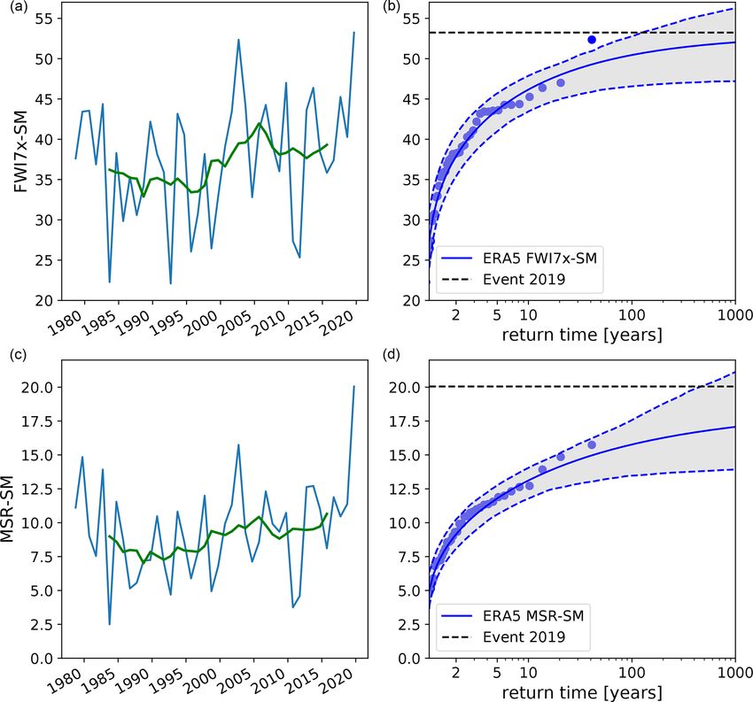
We perform the analysis of possible connections between FWI provides a reasonable proxy for the burned area in the
the fire weather risk and anthropogenic climate change in extended summer months, with the strongest relationship ob-
three steps. First, we assess the trends in extreme temperature served from November to February. Figure 2 shows both the
and conduct an attribution study using the annual maximum Spearman rank correlation and the Pearson correlation of the
of the 7 d moving average of daily maximum temperatures FWI with log-transformed burned area. The 95 % confidence
corresponding to the timescale chosen for the FWI (Sect. 3). intervals are also shown. Given the similarity in the correla-
Second, we undertake the same analysis but for meteorolog- tion coefficients (r) within their confidence intervals, the log-
ical drought (i.e. defined purely as a lack of rainfall) in two linear relationship appears to explain equal variability (r 2 ) to
time windows, the annual precipitation as well as the driest that of the ranks.
month within the fire season, which is September–February To capture spatial variations in the start of the fire season
in our study area (Sect. 4). The latter again roughly corre- at a given location within the event domain, we take for most
sponds to the timescale on which precipitation deficits factor quantities first the maximum per grid point over the fire sea-
into the FWI, namely 52 d. Third, and most importantly, we son (September–February) and next the spatial average over
conduct an attribution study on the FWI and MSR as indices the general event domain. This way the events do not need to
of the probability of bushfires due to the weather (Sect. 5). be simultaneous at separate grid points within the region. We
These three attribution studies follow the same protocol used therefore investigate the question how anthropogenic climate
in previous assessments: heat waves in Kew et al. (2019), low change influences the chances of an intense bushfire season,
precipitation in Otto et al. (2018b), and the Fire Weather In- rather than focusing on a single episode of intense bushfires.
dex in Krikken et al. (2019). The full and generalized event In most years only very small areas are burned, but the ob-
attribution protocol has recently been documented in Philip servational record also includes events with extremely large
et al. (2020). In order to condense the lengthy analysis, we areas. Given this, we checked if the burned-area observations
provide short overviews of the heat and drought analysis in were heavy-tailed (Pasquale, 2013). We found that monthly
the main paper, with extensive results in the Supplement, burned area was not Pareto distributed and instead is reason-
and focus primarily on the FWI and MSR analysis. We also ably approximated using a log-normal distribution. This sup-
provide a short analysis and discussion of other large-scale ports using the log transformation and extrapolating this re-
drivers that were of potential importance during 2019/20, lationship to the 2019/20 fire season. Temporal detrending of
such as El Niño–Southern Oscillation (ENSO), the Indian the observations did not alter these conclusions.
Ocean Dipole (IOD) or the Southern Annular Mode (SAM),
in Sect. 6 with a detailed analysis in Sect. S3. Finally, we 2.2 Observational data
briefly discuss non-climate factors, such as exposure and vul-
nerability, that have contributed to the impacts of the extreme The observational data used in this study are described in
fire season of 2019/20. Sects. S1 and S2 in the Supplement and 5.3 for heat, drought
and the Fire Weather Index, respectively, including justifi-
cations for including or excluding certain datasets for cer-
2 Data and methods tain research questions. For the global mean surface tempera-
ture (GMST) we use GISTEMP (Goddard Institute for Space
2.1 General event definition
Studies Surface Temperature Analysis) surface temperature
Since we are investigating several different indicator or driver (Hansen et al., 2010).
variables of fire risk, different event definitions are devel-
oped for different variables. The details of those definitions 2.3 Model and experiment descriptions
are given at the beginning of the respective sections on tem-
perature, precipitation and fire weather indices (Sects. 3–5). Attributing observed trends to anthropogenic climate change
General parameters of the event definition are given here. can only be done with physical climate models, as they
allow for isolating different drivers. For this purpose we
included as large a set of ocean–atmosphere coupled and
Nat. Hazards Earth Syst. Sci., 21, 941–960, 2021 https://doi.org/10.5194/nhess-21-941-2021G. J. van Oldenborgh et al.: Attribution of the Australian bushfire risk to anthropogenic climate change 945
Figure 2. (a) Correlation between the logarithm of area burned (10 log(km2 ), MODIS Collection 6) in the event domain and the 7 d maximum
Fire Weather Index for each month of the year. The correlations are based on the years 1997 to 2018, and the 95 % two-sided confidence
interval is based on bootstrapping those years. The horizontal line denotes the 5 % significance critical value for a one-sided test of the null
hypothesis that the correlation is zero against the alternative hypothesis that the correlation is positive. (b) Scatterplot and regression line of
the values for each month of the fire season (September–February). The grey lines denote the regression lines for the individual months; the
green line is for all months in the fire season.
atmosphere-only (i.e. sea surface temperature (SST) pre- daily data of relative humidity (RH), temperature, precipita-
scribed) climate model ensembles as we could find within tion and wind speed, the list of models used is shortened to
the time constraints of this study in order to obtain estimates CanESM2, CESM1-CAM5, EC-Earth, IPSL-CM6A-LR and
of both the uncertainty due to natural variability and the weather@home.
model uncertainty. A selection of large ensembles of climate
models from the Coupled Model Intercomparison Project
2.4 Statistical methods
Phase 5 (CMIP5) has been used: CanESM2 (Canadian Earth
System Model), CESM1-CAM5 (Community Earth System
Model–Community Atmosphere Model), CSIRO Mk3.6.0 The methods employed in this analysis have been used pre-
(Commonwealth Scientific and Industrial Research Organ- viously for high and low temperatures (van Oldenborgh
isation), EC-Earth 2.3 (European community earth system et al., 2015; King et al., 2015b; van Oldenborgh et al., 2018;
model), GFDL CM3 (Geophysical Fluid Dynamics Labo- Philip et al., 2018a; Kew et al., 2019), extreme precipita-
ratory Climate Model), GFDL ESM2M (GFDL Earth Sys- tion (Schaller et al., 2014; Siswanto et al., 2015; Vautard
tem Model 2) and MPI-ESM (Max Planck Institute for Me- et al., 2015; Eden et al., 2016; van Oldenborgh et al., 2016;
teorology Earth System Model). In addition, the HadGem3- van der Wiel et al., 2017; van Oldenborgh et al., 2017; Eden
A N216 (Hadley Centre Global Environment Model) attribu- et al., 2018; Otto et al., 2018a; Philip et al., 2018b), drought
tion model developed in the EUropean CLimate and weather (King et al., 2016; Martins et al., 2018; Otto et al., 2018b;
Events: Interpretation and Attribution (EUCLEIA) project, Philip et al., 2018c; Uhe et al., 2018) and forest fire weather
the weather@home (HadAM3P, Hadley Centre atmosphere (Krikken et al., 2019). A paper describing the methods in de-
model) distributed attribution project model, and the ASF- tail was recently published as Philip et al. (2020).
20C (Atmospheric Seasonal Forecasts of the 20th Century) Changes in the frequency of extreme events are calculated
seasonal hindcast ensemble have been used. These last three by fitting the data to a statistical distribution. In this study
models are uncoupled and forced with observed histori- the highest temperature extremes and fire-risk-related vari-
cal SSTs and estimates of SSTs, as they might have been ables (FWI and MSR) of the fire season are assumed to fol-
in a counterfactual world without anthropogenic climate low a generalized extreme value (GEV) distribution, which is
change. Finally, we used the coupled IPSL-CM6A-LR (In- the distribution that block maxima converge to Coles (2001).
stitut Pierre-Simon Laplace Climate Model) low-resolution While our event definition is not exactly block maxima, the
CMIP6 ensemble. The GFDL-CM3 and MPI-ESM models GEV fits the data well (see below for more details). The low
that did not have daily data were not used for the extreme- values of annual mean precipitation and lowest monthly pre-
heat analysis. A list of these climate models and their proper- cipitation of the fire season are fitted using a generalized
ties is given in Table 1. For the FWI analysis, which requires Pareto distribution (GPD), which describes the exceedance
below a low threshold and also allows for the specification of
https://doi.org/10.5194/nhess-21-941-2021 Nat. Hazards Earth Syst. Sci., 21, 941–960, 2021946 G. J. van Oldenborgh et al.: Attribution of the Australian bushfire risk to anthropogenic climate change
Table 1. List of climate model ensembles used.
Name Context Resolution Members Time Reference
ASF-20C seasonal hindcasts T255L91 (0.71◦ ) 51 1901–2010 Weisheimer et al. (2017)
CanESM2 CMIP5 2.8◦ 50 1950–2099 Kirchmeier-Young et al. (2017)
CESM1-CAM5 CMIP5 1◦ 40 1920–2100 Kay et al. (2015)
CSIRO-Mk3-6-0 CMIP5 1.9◦ 30 1850–2100 Jeffrey et al. (2013)
EC-Earth CMIP5 T159 (1.1◦ ) 16 1860–2100 Hazeleger et al. (2010)
GFDL-CM3 CMIP5 2.0◦ 20 1920–2100 Sun et al. (2018)
GFDL-ESM2M CMIP5 2.0◦ 30 1950–2100 Rodgers et al. (2015)
HadGEM3-A attribution N216 (0.6◦ ) 15 1960–2015 Ciavarella et al. (2018)
IPSL-CM6A-LR CMIP6 2.5 × 1.5◦ 32 1950–2019 Boucher et al. (2020)
MPI-ESM CMIP5 1.9◦ 100 1850–2099 Maher et al. (2019)
weather@home attribution N96 (1.8◦ ) 1520 × 2 1987–2017 Guillod et al. (2017)
a threshold that ensures the PDF (probability density func- non-zero, they do not dominate the drought characteristics.
tion) is zero for negative precipitation. Despite these theoretical limitations, in practice the diagnos-
The GEV distribution is tic plots show that the generalized Pareto models are able
" # to describe the data reasonably well. In particular, they re-
x − µ −1/ξ
P (x) = exp − 1 + ξ , (1) spect that precipitation is non-negative. In general this is a
σ difficult problem, and the statistical extremes community is
where x the variable of interest, e.g. temperature or precipi- developing solutions necessary for modelling drought events
tation. Here, µ is the location parameter; σ > 0 is the scale (Naveau et al., 2016).
parameter; and ξ is the shape parameter. The shape parame- To calculate a trend in transient data, some parameters
ter determines the tail behaviour: a negative shape parameter in these statistical models are made a function of the 4-
gives an upper bound to the distribution, for ξ ≥ 1 the tall year smoothed global mean surface temperature (GMST)
is so fat that the mean is infinite. The scale parameter corre- anomaly T 0 . This smoothing is the shortest that on the one
sponds to the variability in the tail. hand reduces the ENSO component of GMST, which is not
The GPD gives a two-parameter description of the tail of externally forced and therefore not relevant for the trend, but
the distribution above a threshold, where the low tail of pre- on the other hand it retains as much of the forced variabil-
cipitation is first converted to a high tail by multiplying the ity as possible (Haustein et al., 2019). A longer smoothing
variable by −1. The GPD is then described by timescale would create problems with extrapolation in the
highly relevant last few years of the instrumental record. The
ξ x (−1/ξ )
covariate-dependent function can be inverted and the dis-
H (u − x) = 1 − 1 − , (2)
σ tribution evaluated for a given year, e.g. a year in the past
with x being the temperature or precipitation, u being the (with T 0 = T00 ) or the current year (T 0 = T10 ). This provides
threshold, σ being the scale parameter, and ξ being the shape estimates and confidence intervals of the probabilities for an
parameter determining the tail behaviour. For the low ex- event at least as extreme as the observed one in these 2 years,
tremes of precipitation, the fit is constrained to have zero p0 and p1 , or expressed as return periods τ0 = 1/p0 and
probability below zero precipitation (ξ < 0, σ < uξ ). Calcu- τ1 = 1/p1 . The change in probability between 2 such years
lations were conducted on the lowest 20 % and 30 % of the is called the probability ratio (PR): PR = p1 /p0 = τ0 /τ1 . We
data, which provide a first-order estimate of the influence of also estimate the changes in intensity (including uncertain-
using more or less extreme events. We cannot use less data, ties): 1T for temperature, 1P for drought and 1FWI.
as the maximizations of the likelihood function do not con- For extreme temperature we assume that the distribution
verge anymore, and using more than 30 % would not qualify shifts with GMST as µ = µ0 + αT 0 or u = u0 + αT 0 and
as the “lower tail”. σ = σ0 with α denoting the trend, which is fitted together
Drought (or low precipitation) is particularly difficult to with µ0 and σ0 . The shape parameter ξ is assumed constant.
model using the existing extreme value framework (Cooley For drought and FWI-related variables we instead make the
et al., 2019). While minima can be modelled by multiplying assumption that the distribution scales with GMST, the scal-
by −1 (Coles, 2001), the applicability of the underlying ex- ing approximation (Tebaldi and Arblaster, 2014). In a GEV
treme value theory assumptions still needs to be validated. In fit this gives
the case of low precipitation, year-on-year autocorrelations
µ = µ0 exp αT 0 /µ0 ,
are a concern. In southeastern Australia, these serial auto-
σ = σ0 exp αT 0 /µ0 ,
correlations are approximately r ≈ 0.2, so although they are (3)
Nat. Hazards Earth Syst. Sci., 21, 941–960, 2021 https://doi.org/10.5194/nhess-21-941-2021G. J. van Oldenborgh et al.: Attribution of the Australian bushfire risk to anthropogenic climate change 947
and in a GPD fit, it is of the distribution the GEV fit agrees with the data points in
the return time plot, as expected from taking block maxima.
u = u0 exp αT 0 /u0 ,
We evaluate all climate models on the fitting parameters
σ = σ0 exp αT 0 /µ0 , by determining whether the model-derived parameters fall
within the uncertainty range of observation-derived parame-
with fit parameters σ0 , α and ξ . The threshold u0 is deter- ters. We allow for a mean bias correction; i.e. we only check
mined with an iterative procedure, and the shape parameter ξ the scale and shape parameters σ and ξ . Model biases are ac-
is again assumed constant. The exponential dependence on counted for by evaluating the model at the same return time
the covariate is in this case just a convenient way to ensure a as the value found in the observational analysis. This was
distribution that is zero for negative precipitation and has no found to give better results than applying an additive or mul-
theoretical justification. For the small trends in this analysis tiplicative bias correction to the position parameter µ, as it
it is similar to a linear dependence. also corrects to first order for biases in the other parameters,
The validity of the other assumption, that the scale param- especially when the distribution has an upper or lower bound
eter or dispersion parameter are constant, is tested by compu- (ξ < 0), which is the case in all the cases here.
tation of the significance of deviation of a constant of running Finally, estimates of the PR and change in observations
(relative) variability plots of the observations and model data and all climate models that pass the evaluation test are com-
(Philip et al., 2020). The analysis of model data is more sen- bined to give a synthesized attribution statement. First, the
sitive to variations of these parameters over time due to the observations and reanalyses were combined by averaging the
large number of ensemble members but of course assumes best estimate and lower and upper bounds, as the natural vari-
the effect of external forcing on the variability is modelled ability is strongly correlated, as they are largely based on the
correctly. same observations (except for the long reanalyses). The dif-
For all fits we also estimate 95 % uncertainty ranges using ference is added as representation uncertainty (white exten-
a non-parametric bootstrap procedure, in which 1000 derived sions on light-blue bars in Figs. S6, S12, S13 and 6).
time series, generated from the original one by selecting ran- Second, the model results were combined by computing
dom data points with replacement, are analysed in exactly the a weighted average (using inverse model total variances), as
same way. The 2.5th and 97.5th percentile of the 1000 output the natural variability in the models, in contrast to the obser-
parameters (defined as 100i/1001 with i being the rank) are vations, is uncorrelated:
taken as the 95 % uncertainty range. For some models with X .X
prescribed SSTs or initial conditions (in the case of the sea- X= Xi /σX2 i 1/σX2 i , (4)
sonal forecast ensemble) the ensemble members are found to i
not be statistically independent, defined here by a correlation with σXi being the estimated uncertainty in model i and Xi
coefficient r > 1/e with e ≈ 2.7182. In those cases the same being either the temperature or the logarithm of precipitation,
procedure is followed except that all dependent time series FWI or MSR. The sums are over the Nmod models. Using this
are entered together in the bootstrapped sample, analogous we can compare the spread expected from the natural vari-
to the method recommended in Coles (2001) to account for ability with the observed spread of the model results using
temporal dependencies. χ 2 statistics:
When using a GEV to model tail behaviour, note that tak-
ing the spatial average of the annual maxima does not have
X .
χ2 = Xi − Xi σXi . (5)
the same statistical justification as taking the annual max- i
imum of the spatial average (Coles, 2001). Given this, the
impact of the order of operations in the event definition was If χ 2 /dof ≤ 1, with dof being the number of degrees of free-
examined. For the temperature extremes, we compared the dom, here N − 1, the spread of the results is compatible
time series where we first take the annual maximum and next with the uncertainty estimated from the fits due to variabil-
the spatial average to the definition with the order reversed, ity within the climate model, and the results can be taken
which can be approximated with a GEV. The Pearson corre- to be independent estimates of X and the weighted average
lation was r = 0.95, which is likely due to strong spatial de- used. However, if χ 2 /dof > 1 the model spread is larger than
pendence and the concentration of heatwaves at the peak of expected from variability due to sampling of weather noise
the seasonal cycle. Therefore, in practice, an approximation alone, so a model spread term was added to each model in ad-
with a GEV is not entirely unsuitable for temperature, but dition to the weighted average (white extensions on the light-
caution should be exercised. For the FWI and MSR, the order red bars, Figs. S5 and S6) to account for systematic model
of operations does make a clear difference. Indeed, we find errors. This term is defined by requiring that χ 2 /dof = 1.
that the whole distribution is not described well by a GEV The total uncertainty of the models is shown as a bright-
for one climate model used (CanESM2). For that model we red bar in these figures. This total uncertainty consists of a
take block maxima over five ensemble member blocks, effec- weighted mean using the uncorrelated natural variability plus
tively looking only at the most extreme events. For this part an independent model spread term added to the uncertainty
https://doi.org/10.5194/nhess-21-941-2021 Nat. Hazards Earth Syst. Sci., 21, 941–960, 2021948 G. J. van Oldenborgh et al.: Attribution of the Australian bushfire risk to anthropogenic climate change
√
if χ 2 /dof > 1, which we do not divide by N − 1; i.e. we Given the larger trend in observations than in the models we
do not assume that by adding more models to the ensemble suspect that climate models underestimate the trend in ex-
the model uncertainty decreases. This procedure is similar to treme temperatures due to climate change, although in prin-
the one employed by Ribes et al. (2020). ciple the difference could also be due to a non-climatic driver
Finally, observations and models are synthesized into a that affects the trend in observations. The combination of a
single mean and uncertainty range. This can only be done weaker trend and higher variability in models compared to
when they appear to be compatible. We show two combi- observations yields an increase in the likelihood of such an
nations. The first one is computed by neglecting model un- event that is much higher in observations than in models.
certainties beyond the model spread. The optimal combina-
tion is then the weighted average of models and observations,
shown as a magenta bar. However, the total model uncer- 4 Meteorological drought
tainty is unknown and can be larger than the model spread.
We therefore also show the more conservative estimate of an The key takeaways from the attribution analysis of trends
unweighted average of observations and models with a white in low precipitation are summarized here, while the details
box in the synthesis plots. are given in Sect. S2. The conclusions below are shown in
Fig. S12 for annual mean drought, and those in Fig. S13 are
for the driest month of the year.
3 Extreme heat Observations show non-significant trends towards more
dry extremes like the record 2019 annual mean and a non-
The key takeaways from the attribution analysis of trends in significant trend towards fewer dry months like Decem-
extreme heat are summarized here, while the details are given ber 2019 in the fire season (Figs. S12 and S13). All 10 cli-
in Sect. S1. mate models we considered simulate the statistical proper-
Taking advantage of the longer observational record for ties of the observations well (Figs. S10 and S11). Collec-
temperature than for other variables, we analyse the highest tively they show trends neither in dry extremes of annual
7 d mean maximum temperatures of the year (TX7x), aver- mean precipitation nor in the driest month of the fire sea-
aged over the event domain (Fig. 1), from 1910 (the begin- son (September–February). We conclude that there is no ev-
ning of standardized temperature observations) to 2019. idence for an attributable trend in either kind of meteorolog-
Observations show that a heatwave as rare as observed ical drought extremes like the ones observed in 2019.
in 2019/20 would have been 1 to 2 ◦ C cooler at the beginning
of the 20th century (Fig. S6). Similarly, a heatwave of this
5 Fire risk indices
intensity would have been less likely by a factor of about 10
in the climate around 1900 (Fig. S6). While climate mod- 5.1 The fire weather of 2019/20
els consistently simulate increasing temperature trends over
this time period, they all have some limitations for simulating As discussed in the introduction, the fire risk as described
heat extremes: the variability of 7 d mean maximum temper- by fire weather indices was extreme in the study domain in
ature is generally too high, and the long-term trend is only the 2019/20 fire season. The domain was chosen to encom-
1 ◦ C (Figs. S5 and S6). We can therefore only conclude that pass these fires, and therefore the 2019/20 event cannot be
anthropogenic climate change has made a hot week like the included in the statistical analysis.
one in December 2019 more likely by at least a factor of 2 but
cannot give a best estimate or upper bound due to the model 5.2 Temporal event definition
deficiencies limiting our confidence in the exact magnitude
of the anthropogenic influence. We choose two event definitions in order to represent two
The reasons for the apparent model deficiencies in simu- important aspects of the event, namely the intensity and the
lating trends and variability in extreme temperatures are not duration. For intensity, we first select the maximum FWI
fully understood. In Sect. S3 we show that the temperature of a 7 d moving average over the fire season (September–
variability explained by the Indian Ocean Dipole (IOD) and February) for every grid point over the study region, after
Southern Annual Mode (SAM) is too small to explain these which we compute the spatial average, hereafter FWI7x-SM
mismatches as problems in the model representation of these (seasonal maximum). The 7 d timescale was chosen based on
modes of variability. The literature suggests that shortcom- a good correlation with the area burned (see Fig. 2) and good
ings in the coupling to land and vegetation (e.g. Fischer et al., correspondence with area burned in other forest fire attribu-
2007; Kala et al., 2016) and in parametrization of irrigation tions studies (Krikken et al., 2019).
(e.g. Thiery et al., 2017; Mathur and AchutaRao, 2019) in the For duration, we consider the monthly severity rat-
exchange of heat and moisture with the atmosphere and also ing (MSR). The MSR is the monthly averaged value of the
in the representation of the boundary layers (e.g. Miralles daily severity rating (DSR), which in turn is a transforma-
et al., 2014) are more likely to be the cause of the problems. tion of the FWI (DSR = 0.0272FWI1.71 ). The DSR reflects
Nat. Hazards Earth Syst. Sci., 21, 941–960, 2021 https://doi.org/10.5194/nhess-21-941-2021G. J. van Oldenborgh et al.: Attribution of the Australian bushfire risk to anthropogenic climate change 949
better how difficult a fire is to suppress, while the MSR the 1.1 ◦ C temperature increase for the present-day climate
is a common metric for assessing fire weather on monthly and the 2 ◦ C increase for the future reference climate and
timescales (Van Wagner, 1970). For this study, we select the not 2019 and 2060. As the fits are invariant under a scaling
maximum value of the MSR during the fire season over the of the covariate, this does not make much difference.
study area (MSR-SM). In contrast to the FWI7x-SM, we First the models are evaluated on how well they represent
first apply a spatial average of the study area and then se- the extremes of the FWI7x-SM and MSR-SM. This is quanti-
lect the maximum value per fire season. This event defini- fied by the dispersion parameter σ/µ and shape parameter ξ
tion focuses more on changes in extreme fire weather for of the GEV fit for the present-day climate. We do not check
longer timescales and larger integrated areas than FWI7x- the position parameter µ, assuming a multiplicative bias cor-
SM. Note that neither of the two event definitions includes rection can be applied.
ignition sources or small-scale meteorological factors such Figure 5 gives an overview of these parameters. Prefer-
as pyrocumulonimbus development that could enhance the ably, we would like the parameters to lie within the obser-
fires. vational uncertainty of ERA5. For the dispersion parameter
CanESM2 and weather@home fall within the observational
5.3 Observational analysis: return time and trend uncertainty of the FWI. The other two models (EC-Earth and
IPSL CM6) show too much variability relative to the mean.
For the observational analysis we use the fifth-generation The same holds for the shape parameter. This implies that it
European Centre for Medium-Range Weather Fore- is difficult to draw strong conclusions from the model data,
casts (ECMWF) Atmospheric Reanalysis (ERA5) dataset given that they do not accurately represent the extremes of
for 1979–January 2020 (Hersbach et al., 2019). This reanal- the FWI7x-SM. In particular, the models with too much vari-
ysis dataset is heavily constrained by observations and thus ability will underestimate the probability ratios. We continue
provides one of the best estimates of the actual state of the with all four models but keep these problems in mind.
atmosphere for all the variables needed to compute the FWI The MSR is simulated better: all model dispersion and
over the study area. Other reanalyses did not yet include the shape parameters lie within the large observational uncertain-
full 2019/20 event at the time of the analysis. ties, although they largely disagree with one another on the
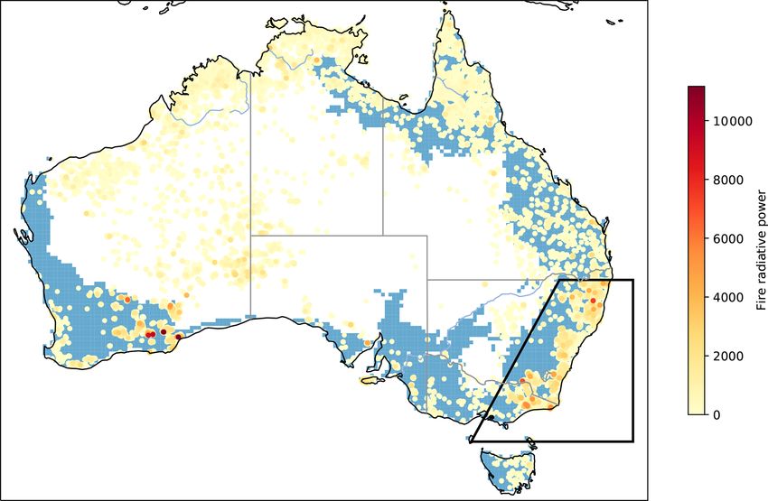
Figure 3 shows the time series of the highest 7 d mean FWI dispersion parameter.
averaged over the study area. Both for the FWI7x-SM and
MSR-SM the event is the highest over the 1979–2020 time
5.5 Multi-model attribution and synthesis
period. Note that for the MSR-SM, the value is considerably
more extreme than for the FWI7x-SM. The GEV fits (Fig. 3,
right) illustrate this further, with return times in excess of The model results are summarized by their PR, i.e. how more
1000 years. or less likely such an event will be for present or future cli-
A fit allowing for scaling with the smoothed GMST gives mate, relative to the early 20th century.
a significant trend in the FWI7x-SM (Fig. 4). This fit gives Figures 6 and 7 show the change in probability for both
a return time for the 2019/20 fire season of about 31 years the FWI7x-SM and the MSR-SM from 1920 to 2019 (denot-
(4 to 500 year) in the current climate and more than 800 years ing the 2019/20 fire season). For the FWI7x-SM, all mod-
extrapolated to the climate of 1900. This corresponds to an els agree on an increased probability for such an event in the
infinite PR, with a lower bound of 4. The return time for the present climate relative to the early 20th century, although the
MSR-SM is undefined and is thus estimated to be 100 years. trend is not significant at p < 0.05 (two-sided) for one of the
For the climate model analysis we thus use return times of models, CanESM2. As the spread of the models is compati-
31 years for the FWI7x-SM and 100 years for the MSR-SM ble with natural variability (χ 2 /dof < 1), we take a weighted
to determine the event thresholds in individual climate mod- average across the models to synthesize them (Fig. 6). This
els. shows that such an event has become about 80 % more likely
in the models, with a lower bound of 30 %. Note that all
5.4 Model evaluation models severely underestimate the increased risk compared
to ERA5, which has a lower bound of the PR of a factor
We use four climate models with large ensembles, leaving of 4 relative to 1920 (extrapolated), above the upper end of
out CESM1-CAM5 because of its failure to represent heat the model average. Note that the ERA5 value is probably bi-
extremes (see Sect. 3). This is fewer than for the drought ased high, as the positive contribution of trend towards a drier
and heat analysis because the FWI requires four daily in- climate over 1979–2019 is not present over 1900–2019; see
put variables, which are not available for all models. In con- Sects. S2 and 5.6.
trast to the heat extremes and drought analyses, the fits to For a future climate of 2 ◦ C warming above pre-industrial
the model output use as covariate the model GMST. We also levels we find that such events become about 8 times more
define our reference climates using GMST rather than years. likely in the models, with a lower bound of about 4 times
The years at which the climate is evaluated are taken from more likely. Note that the estimate of future climate is only
https://doi.org/10.5194/nhess-21-941-2021 Nat. Hazards Earth Syst. Sci., 21, 941–960, 2021950 G. J. van Oldenborgh et al.: Attribution of the Australian bushfire risk to anthropogenic climate change
Figure 3. (a, c) Time series with the 10-year running mean of the area average of the highest 7 d mean Fire Weather Index in September–
February (a) and maximum of the monthly severity rating in September–February (c). (b, d) Stationary GEV fit to these data; the dots
represent the ordered years, and the grey bands represent the 95 % uncertainty ranges.
based on two climate models, CanESM2 and EC-Earth, due in some models is reminiscent of the extreme-temperature
to the absence of future data for the others. results in Sects. 3 and S1.
For the MSR-SM the models on average show about a In order to better understand which input variables cause
doubling of probability for the present climate relative to the the long-term increase in the FWI7x-SM and thus the con-
early 20th century (Fig. 7). However, this trend is not signif- tribution to the 2019/20 FWI7x-SM value, we study the in-
icant, as the lower bound is 0.8; i.e. a decreased probability put variables to the FWI7x-SM separately for each model as
is also possible within the two-sided 95 % uncertainty range. well as observations. For precipitation we use the cumulative
In the fit to the ERA5 data we include 2019, as otherwise precipitation (90 d) prior to each FWI7x-SM value. We cal-
the probability of the event occurring in the current climate culate the change from the early 20th century to the present
would be zero, contrary to the fact that it did occur. This fit day in each input variable to estimate its long-term change,
shows much higher probability ratios, with a lower bound which we then subtract from that variable’s observed value
of a factor of 9. As there is no overlap with the model re- in 2019/20. We then recalculate the FWI7x-SM but use each
sults we cannot combine the model and observational results detrended individual input variables in turn. Each of these
but only give a conservative lower bound as an observation– newly calculated FWI7x-SM values thus illustrates the in-
model synthesis result. For a future climate relative to the cli- fluence of the long-term trend in a particular input variable
mate of the early 20th century the models show an increase onto the observed 2019/20 FWI7x-SM value. This proce-
in probability of about 4 times, with a lower bound of 2. dure is applied to models and ERA5. In the models, the en-
semble mean change is used to estimate an individual vari-
able’s long-term trend, whereas in ERA5 a regression of
5.6 Interpretation
each variable onto GMST is used to estimate its value in
the early 20th century. The results of this analysis for the
The underestimation of the observed trend in fire weather in- 2019/20 FWI7x-SM value are shown in Fig. 9.
dices in all models and the tendency for too much variability
Nat. Hazards Earth Syst. Sci., 21, 941–960, 2021 https://doi.org/10.5194/nhess-21-941-2021G. J. van Oldenborgh et al.: Attribution of the Australian bushfire risk to anthropogenic climate change 951
In ERA5 the increase in temperature also appears to be
the most important explanatory variable, followed by a de-
crease in RH and precipitation. As we did not find a signif-
icant trend in precipitation over longer time periods, we hy-
pothesize this trend to be due to natural variability over the
short 1979–2018 period in ERA5. We explicitly verified that
the dependence of the FWI7x-SM on temperature is almost
linear in a range of ±5 K around the reanalysis value (not
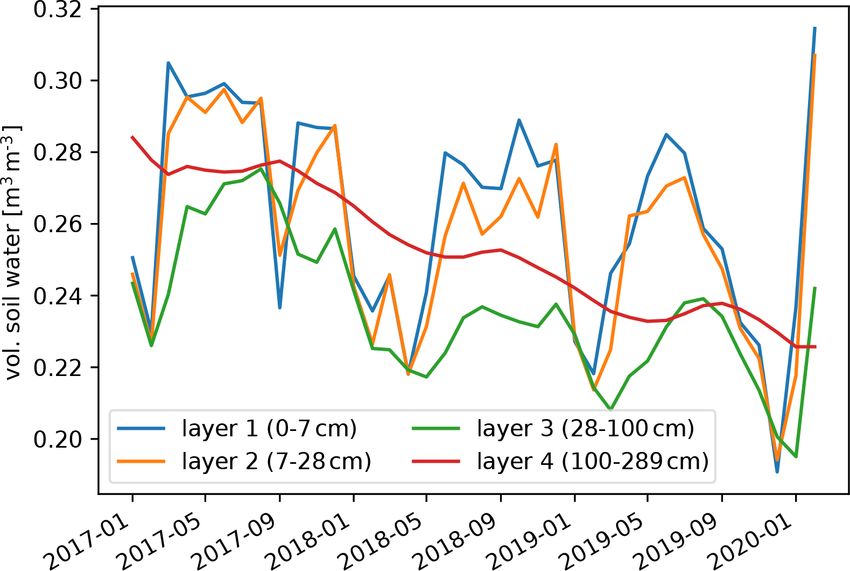
shown). Further, volumetric soil water (Fig. 8) at multiple
soil layers from ERA5 suggests that, despite the soil already
being very dry in 2018 and into 2019, the 2019/20 austral
spring–summer drought caused a further drying of the soil in
the study area. This suggests that the drought of late 2019 and
high temperatures did indeed cause an additional increase in
fire risk over preceding years.
5.7 Conclusions fire risk indices
The FWI7x-SM as computed from the ERA5 reanalysis as an
approximation to the real world shows that the 2019/20 val-
ues were exceptional. They have a significant trend towards
higher fire weather risk since 1979. Compared with the cli-
mate of 1900, the probability of an FWI7x-SM as high as
in 2019/20 has increased by more than a factor of 4. For the
MSR-SM the probability has increased by more than a factor
Figure 4. Fit of a GEV that scales with the smoothed GMST (Eqs. 1 of 9.
and 3) of the highest 7 d mean FWI computed from the ERA5 re- The four climate models investigated show that the prob-
analysis, averaged over the index region. (a) Observations (blue
ability of a Fire Weather Index this high has increased by at
symbols), location parameter µ (thick line and uncertainties in 1900
(extrapolated) and 2019/20), and the 6 and 40 year return values least 30 % since 1900 as a result of anthropogenic climate
(thin lines). The purple square denotes the 2019/20 value, which is change. As the trend in extreme temperature is a driving fac-
not included in the fit. (b) Return time plot with fits for the climates tor behind this increase and the climate models underestimate
of 1900 (blue lines with 95 % confidence interval) and 2019 (red the observed trend in extreme temperature, the attributable
lines); the purple line denotes the 2019/20 event. The observations increase in fire risk could be much higher. This is also re-
are plotted twice, shifted down to the climate of 1900 (blue stars) flected by a larger trend in the FWI7x-SM in the reanaly-
and up to the climate of 2019 (red pluses) using the fitted depen- sis compared to models. The MSR-SM increased by a factor
dence on smoothed global mean temperature so that they can be of 2 in the models since 1900, although this increase is not
compared with the fits for those years. significantly different from zero. As with FWI7x-SM, the at-
tributable increase is likely higher due to the model under-
estimation of temperature trends and overestimation of vari-
The sum of the contributions from individual input vari-
ability in the TX7x.
ables to the 2019/20 FWI7x-SM anomaly match the effect
Projected into the future, the models project that an
of changing all variables at the same time, so they can be
FWI7x-SM as high as in 2019/20 would become at least
considered linearly additive (Fig. 9). The underestimation of
4 times more likely with a 2 ◦ C temperature rise, compared
the extreme-temperature trends in the climate models carries
with 1900. Due to the model limitations described above this
over into this analysis such that the temperature contribu-
could also be an underestimate.
tion to the observed 2019/20 value is underestimated. De-
spite this underestimation, temperature emerges as the most
important variable in EC-Earth and weather@home, as it ex-
plains roughly half of the increase in the FWI. For IPSL, the 6 Other drivers
simulated temperature increase explains about a third of the
The attribution statements presented in this paper are for
FWI7x-SM increase, together with wind and RH. CanESM2
events defined as meeting or exceeding the threshold set
behaves differently, where it is mainly the decrease of RH
by the 2019/20 fire season and thus assessing the overall
that explains the higher FWI7x-SM. Most but not all models
effect of human-induced climate change on these kinds of
analysed here therefore derive the increase in the FWI7x-SM
events. In individual years, however, large-scale climate sys-
largely from the increase in temperature extremes.
tem drivers can have a higher influence on fire risk than the
https://doi.org/10.5194/nhess-21-941-2021 Nat. Hazards Earth Syst. Sci., 21, 941–960, 2021952 G. J. van Oldenborgh et al.: Attribution of the Australian bushfire risk to anthropogenic climate change
Figure 5. Model verification for the FWI (a, b) and MSR (b, c). The left figures show the dispersion parameter σ/µ, and the right figures
show the shape parameter ξ . The bars denote the 95 % uncertainty ranges.
Figure 6. (a) The PR for an FWI as high as observed in 2019/20
Figure 7. As Fig. 6 but for the monthly severity rating (MSR).
or higher: (a) from 1920/21 to 2019/20 and (b) from 1900 to a cli-
mate globally 2 ◦ C warmer than 1920. The last row is the weighted
average of all models, the spread of which is consistent with only
natural variability. (b) Same for a 2 ◦ C climate (GMST change from
the late 19th century).
trend. A detailed analysis of the influence of ENSO, the IOD
and SAM is presented in Sect. S3.
Besides the influence of anthropogenic climate change,
the particular 2019 event was made much more severe by
a record positive excursion of the Indian Ocean Dipole and
a very strong negative anomaly of the Southern Annular
Mode, which likely contributed substantially to the precip-
itation deficit. We did not find a connection of either mode to
heat extremes. More quantitative estimates will require fur- Figure 8. ERA5 volumetric soil water from multiple levels. The
ther analysis and dedicated model experiments, as the linear- data represent the spatial average over the study area. Please note
ity of the relationship between these indices and the regional that the date format in this figure is year month (yyyy-mm).
climate is not verifiable from observations alone.
Nat. Hazards Earth Syst. Sci., 21, 941–960, 2021 https://doi.org/10.5194/nhess-21-941-2021G. J. van Oldenborgh et al.: Attribution of the Australian bushfire risk to anthropogenic climate change 953
Figure 9. Sensitivity analysis of the FWI7x-SM to changes in individual contributions from relative humidity (RH, wind, temperature and
precipitation). The relative increases or decreases for the individual variables of the climate models are based on the average change in input
variables between the climate of the present day and the early 20th century (values above bars). For ERA5 the changes are based on a linear
regression of the respective variable onto GMST for the years 1979 to 2018 and then extrapolated to the early 20th century. These changes
are subtracted from the 2019 ERA5 data, after which the FWI is recomputed, where 1FWI is the original FWI minus the altered FWI.
In the “all” experiment all input variables are changed simultaneously. “Sum” is the sum of all the individual changes in the FWI. W@H:
weather@home.
7 Vulnerability and exposure individual or group to anticipate, cope with, resist and
recover from the impact of a natural or man-made hazard”
At least 19.4 × 10⁶ ha of land has burned as a result (https://www.ifrc.org/en/what-we-do/disaster-management/
of the Black Summer bushfires of 2019/20 (https:// about-disasters/what-is-a-disaster/what-is-vulnerability/,
disasterphilanthropy.org/disaster/2019-australian-wildfires/, last access: 7 March 2021). Exposure is defined as “The
last access: 6 March 2021). This has resulted in 34 di- presence of people, livelihoods, species or ecosystems, envi-
rect deaths and the destruction of 5900 residential and ronmental functions, services, and resources, infrastructure,
public structures (https://reliefweb.int/report/australia/ or economic, social, or cultural assets in places and settings
australia-bushfires-information-bulletin-no-4, last ac- that could be adversely affected” (Agard et al., 2014).
cess: 7 March 2021). Nearly 80 % of Australians re- Bushfires have been a part of the Australian landscape for
ported being impacted in some way by the bushfires millions of years and are an ever-present risk for people liv-
(https://theconversation.com/nearly-80-of-australians- ing in rural and peri-urban areas surrounded by vegetation,
affected-in-some-way-by-the-, last access: 7 March 2021). bush and/or grasslands. In recent decades, significant bush-
In Sydney, Canberra and a number of other cities, air fires occurred in 1974/75, 1983, 2002/03 and 2009, some of
quality levels of towns and communities reached hazardous them including grass fires, which can have different drivers
levels (https://www.nytimes.com/interactive/2020/01/03/ to forest fires like those in 2019/20. This frequent occurrence
climate/australia-fires-air.html, last access: 7 March 2021). of severe bushfires, with records extending back to the 1850s,
Over 65 000 people registered on Australian Red Cross’ has resulted in robust preparedness and emergency manage-
reunification site to look for friends and family or to let loved ment systems which serve to reduce risk and aid in swift re-
ones know that they were alright (https://www.redcross.org. sponse. Comprehensive risk assessments are undertaken at
au/news-and-media/news/bushfire-response-20-feb-2020, the level of the local council, and bushfire preparedness and
last access: 7 March 2021). It is estimated that over contingency plans have been in place in most high-risk areas
1.5 billion animals have died nationally (https://reliefweb. for decades. However, these systems were severely strained
int/sites/reliefweb.int/files/resources/IBAUbf050220.pdf, in the Black Summer bushfires.
last access: 7 March 2021). These impacts are not only
hazard-related but also related to various vulnerability 7.1 Excess morbidity and mortality
and exposure factors that each play a role in increasing
or decreasing risk and impacts. Vulnerability is defined as The time of publication is too soon for a robust estimate of
“The propensity or predisposition to be adversely affected. excess morbidity and mortality specific to the 2019/20 Aus-
Vulnerability encompasses a variety of concepts and ele- tralian bushfires. Such analysis is typically available weeks
ments including sensitivity or susceptibility to harm and to years following the end of an event. However, the
lack of capacity to cope and adapt” (Agard et al., 2014). combined impacts of extreme heat and air pollution can be
It can also be defined as “the diminished capacity of an deadly, as seen in the compounded heatwave and wildfire
https://doi.org/10.5194/nhess-21-941-2021 Nat. Hazards Earth Syst. Sci., 21, 941–960, 2021You can also read