AEROCOM and AEROSAT AAOD and SSA study - Part 1: Evaluation and intercomparison of satellite measurements - Recent
←
→
Page content transcription
If your browser does not render page correctly, please read the page content below

Atmos. Chem. Phys., 21, 6895–6917, 2021
https://doi.org/10.5194/acp-21-6895-2021
© Author(s) 2021. This work is distributed under
the Creative Commons Attribution 4.0 License.

AEROCOM and AEROSAT AAOD and SSA study – Part 1:
Evaluation and intercomparison of satellite measurements
Nick Schutgens1 , Oleg Dubovik2 , Otto Hasekamp3 , Omar Torres4 , Hiren Jethva5 , Peter J. T. Leonard6 ,
Pavel Litvinov2 , Jens Redemann7 , Yohei Shinozuka8,9 , Gerrit de Leeuw10,a , Stefan Kinne11 , Thomas Popp12 ,
Michael Schulz13 , and Philip Stier14
1 Department    of Earth Science, Vrije Universiteit Amsterdam, 1081 HV Amsterdam, the Netherlands
2 Laboratoire  d’Optique Atmosphérique, CNRS/Université de Lille, Villeneuve-d’Ascq, France
3 Netherlands Institute for Space Research (SRON), Utrecht, the Netherlands
4 Atmospheric Chemistry and Dynamics Laboratory, NASA Goddard Space Flight Center, Greenbelt, MD 20771, USA
5 Universities Space Research Association – GESTAR, NASA Goddard Space Flight Center, Greenbelt, MD 20771, USA
6 ADNET Systems, Inc., Suite A100, 7515 Mission Drive, Lanham, MD 20706, USA
7 School of Meteorology, University of Oklahoma, Norman, USA
8 Universities Space Research Association, Columbia, Maryland, USA
9 NASA Ames Research Center, Moffett Field, California, USA
10 Finnish Meteorological Institute (FMI), Climate Research Programme, Helsinki, Finland
11 Max-Planck-Institut für Meteorologie, 20146 Hamburg, Germany
12 German Aerospace Center (DLR), German Remote Sensing Data Center Atmosphere, Oberpfaffenhofen, Germany
13 Norwegian Meteorological Institute, P.O. Box 43, Blindern, 0313 Oslo, Norway
14 Atmospheric, Oceanic and Planetary Physics, Department of Physics, University of Oxford, Oxford, UK
a currently at: Royal Netherlands Meteorological Institute (KNMI), R&D Satellite Observations, De Bilt, the Netherlands

Correspondence: Nick Schutgens (n.a.j.schutgens@vu.nl)

Received: 23 November 2020 – Discussion started: 7 December 2020
Revised: 23 February 2021 – Accepted: 8 March 2021 – Published: 6 May 2021

Abstract. Global measurements of absorbing aerosol optical        how minimum AOD (aerosol optical depth) thresholds and
depth (AAOD) are scarce and mostly provided by the ground         temporal averaging may improve agreement between satel-
network AERONET (AErosol RObotic NETwork). In recent              lite observations.
years, several satellite products of AAOD have been devel-           All satellite datasets are shown to have reasonable skill
oped. This study’s primary aim is to establish the usefulness     for AAOD (three out of four datasets show correlations with
of these datasets for AEROCOM (Aerosol Comparisons be-            AERONET in excess of 0.6) but less skill for SSA (single-
tween Observations and Models) model evaluation with a fo-        scattering albedo; only one out of four datasets shows cor-
cus on the years 2006, 2008 and 2010. The satellite products      relations with AERONET in excess of 0.6). In comparison,
are super-observations consisting of 1◦ × 1◦ × 30 min aggre-      satellite AOD shows correlations from 0.72 to 0.88 against
gated retrievals.                                                 the same AERONET dataset. However, we show that per-
   This study consists of two papers, the current one that        formance vs. AERONET and inter-satellite agreements for
deals with the assessment of satellite observations and a sec-    SSA improve significantly at higher AOD. Temporal aver-
ond paper (Schutgens et al., 2021) that deals with the eval-      aging also improves agreements between satellite datasets.
uation of models using those satellite data. In particular, the   Nevertheless multi-annual averages still show systematic dif-
current paper details an evaluation with AERONET obser-           ferences, even at high AOD. In particular, we show that two
vations from the sparse AERONET network as well as a              POLDER (Polarization and Directionality of the Earth’s Re-
global intercomparison of satellite datasets, with a focus on     flectances) products appear to have a systematic SSA differ-

Published by Copernicus Publications on behalf of the European Geosciences Union.
6896                                      N. Schutgens et al.: AEROCOM and AEROSAT AAOD and SSA study – Part 1

ence over land of ∼ 0.04, independent of AOD. Identifying            Currently, absorbing aerosol can be measured in a num-
the cause of this bias offers the possibility of substantially    ber of ways. AERONET (AErosol RObotic NETwork, Hol-
improving current datasets.                                       ben et al., 1998) is a global but spatially sparse network of
   We also provide evidence that suggests that evaluation         Sun photometers that includes two scanning protocols (al-
with AERONET observations leads to an underestimate of            mucantar and hybrid) that allow the inversion of measured
true biases in satellite SSA.                                     radiances into particle size distributions and refractive in-
   In the second part of this study we show that, notwith-        dices (Dubovik and King, 2000). From this inversion, colum-
standing these biases in satellite AAOD and SSA, the              nar AAOD (absorbing aerosol optical depth) can be derived.
datasets allow meaningful evaluation of AEROCOM mod-              There are also networks (Laj et al., 2020) of (filter-based) ab-
els.                                                              sorption photometers, as used in EMEP (European Monitor-
                                                                  ing and Evaluation Programme), ACTRIS (Aerosol, Clouds
                                                                  and Trace Gases Research Infrastructure) and IMPROVE
1   Introduction                                                  (Interagency Monitoring of Protected Visual Environments).
                                                                  These networks are concentrated in Europe and North Amer-
Aerosol is an important component of the Earth’s atmosphere       ica, and there is no global coverage. Moreover, these are
that affects the planet’s climate, the biosphere and human        surface measurements that do not measure the full atmo-
health. Aerosol particles scatter and absorb sunlight as well     spheric column. Finally, absorption photometers like the SP2
as modify clouds. Anthropogenic aerosol changes the ra-           were used on flight campaigns like HIPPO (Schwarz et al.,
diative balance and influences global warming (Angstrom,          2010, 2013; Wang et al., 2014). Again, this yields spatially
1962; Twomey, 1974; Albrecht, 1989; Hansen et al., 1997;          sparse in situ observations of absorbing aerosol. While these
Lohmann and Feichter, 1997, 2005). It may negatively af-          measurement networks have proven to be very important to
fect solar power generation (Li et al., 2017; Labordena et al.,   our understanding of absorbing aerosol, a satellite-derived
2018). Aerosol can transport soluble iron, phosphate and ni-      AAOD would contribute greatly by adding spatial context in
trate over long distances and provide nutrients for the bio-      regions with ground-based instruments and measurements in
sphere (Swap et al., 1992; Vink and Measures, 2001; Mc-           regions without such instruments. As it now stands, we have
Tainsh and Strong, 2007; Maher et al., 2010; Lequy et al.,        almost no observations of absorbing aerosol over the oceans,
2012) . Aerosol can penetrate deep into lungs and may carry       in particular in continental outflow regions.
toxins or serve as disease vectors (Dockery et al., 1993;            However, in recent years a number of satellite AAOD
Brunekreef and Holgate, 2002; Ezzati et al., 2002; Smith          products have been developed, often based on POLDER
et al., 2009; Beelen et al., 2013; Ballester et al., 2013).       (Polarization and Directionality of the Earth’s Reflectances)
   Aerosol reflects visible radiation from the Sun, and some      measurements. For example, Lacagnina et al. (2015) used
aerosol also absorbs it (Dubovik et al., 2002; Omar et al.,       POLDER data to evaluate SSA (single-scattering albedo)
2005). The species that absorb the most visible sunlight are,     from AEROCOM (Aerosol Comparisons between Observa-
in order of importance, black carbon, dust and brown car-         tions and Models) models over oceans, Peers et al. (2016)
bon. Of these, black carbon is expected to exert a significant    evaluated over ocean above-cloud SSA in AEROCOM mod-
positive radiative forcing on the climate (Bond et al., 2013;     els for the African fire season, Lacagnina et al. (2017) es-
Myhre et al., 2013). Absorbing aerosol’s impact is mostly         timated the global direct radiative effect of aerosol, and
through heating of the atmospheric profile (direct effect) and    Hasekamp et al. (2019b) estimated aerosol–cloud interac-
subsequent stabilization or destabilization (Johnson et al.,      tions. Chen et al. (2018, 2019) assimilated POLDER AOD
2003) of the boundary layer (semi-direct effect). This affects    and AAOD observations to estimate aerosol emissions, while
cloud formation (Koren et al., 2008; Brioude et al., 2009) and    Tsikerdekis et al. (2021) showed the benefit of jointly assimi-
precipitation (Hodnebrog et al., 2016; Samset et al., 2016;       lating POLDER AOD (aerosol optical depth), AE (Ångström
Hodzic and Duvel, 2018). In particular over bright surfaces       exponent) and SSA (single-scattering albedo) observations.
(ice, deserts, clouds) the forcing due to absorbing aerosol can   Kacenelenbogen et al. (2019) used combinations of A-Train
be significant (Haywood and Shine, 1995; Graaf et al., 2012;      sensors to infer AAOD over clouds and estimate short-wave
Tegen and Heinold, 2018).                                         direct aerosol effects.
   On regional scales, biomass burning smoke has been im-            The challenge in retrieving AAOD from satellites is made
plicated in increased tornado severity (Saide et al., 2015),      clear by the challenge in retrieving AAOD from AERONET
while dust was observed to reduce cyclones (Chen et al.,          measurements. AERONET AAOD observations are known
2017); black carbon may affect the Hadley cell circulation        to be more uncertain than AOD observations. Dubovik et al.
(Allen et al., 2012; Tosca et al., 2013); and black carbon        (2000) estimated that AERONET SSA uncertainties for AOD
deposition can reduce glacier albedo (Thomas et al., 2017;        ≤ 0.2 at 440 nm would be at least 0.05, using numerical sen-
Zhang et al., 2017; Dang et al., 2017), which may speed up        sitivity tests. A recent in-depth estimate of the uncertainty
glacier melt.                                                     in Inversion V3 data (Sinyuk et al., 2020) for four differ-
                                                                  ent sites suggested SSA uncertainties at AOD (at 440 nm)

Atmos. Chem. Phys., 21, 6895–6917, 2021                                             https://doi.org/10.5194/acp-21-6895-2021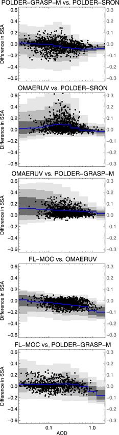
N. Schutgens et al.: AEROCOM and AEROSAT AAOD and SSA study – Part 1                                                              6897

equal 0.2 from 0.037 to 0.048 at 440 nm and from 0.035 to
0.045 at 675 nm. It is not clear whether these uncertainties
should be interpreted as site-specific biases or random er-
rors. This distinction matters as random errors can be reduced
through appropriate averaging of data. Large differences be-
tween AERONET SSA at low AOD and in situ measure-
ments were indeed confirmed by Andrews et al. (2017). Even
at higher AOD (≥ 0.5), Dubovik et al. (2000) suggested SSA
errors of at least 0.03. Sinyuk et al. (2020) suggest smaller
SSA uncertainties of 0.017 to 0.023 at 440 nm and 0.015 to
0.026 at 675 nm for AOD (at 440 nm) equal to 0.6. Given the
challenges in satellite remote sensing compared to ground-
based remote sensing, satellite AAOD and SSA products can
be expected to have large errors as well.
   Global Climate Observing System (GCOS) requirements
                                                                   Figure 1. Colour legend used throughout this paper to designate the
(WMO, 2011) for SSA specify an accuracy within 0.03 and            different satellite products for both this study and the AOD study in
a stability per decade within 0.01, for a horizontal resolution    Schutgens et al. (2020).
of 5–10 km and a temporal resolution of 4 h. These require-
ments appear based on typical regional and yearly variations
in SSA. However, SSA requirements are different for differ-        groups. They meet every year to discuss common issues in
ent applications (monitoring, trends, model evaluation, pro-       the field of aerosol studies.
cess studies), while the GCOS requirements are meant to pro-          The observational datasets used in this study are described
vide a general broad estimate (Popp et al., 2016). In part 2 of    in Sect. 2. The collocation and analysis methodology are de-
our study we will show that current satellite AAOD and SSA         scribed in Sect. 3. A first look at the satellite datasets is pre-
capabilities allow for useful evaluation of models.                sented in Sect. 4. Evaluation of satellite AOD, AAOD and
   For measurements to be useful in model evaluation, their        SSA with AERONET is performed in Sect 5, and a more de-
errors after averaging (spatially, temporally) need to be          tailed intercomparison of satellite data is shown in Sect. 6. A
smaller than the model errors the observations should be able      summary and conclusions can be found in Sect. 7.
to identify. A traditional evaluation of satellite datasets with
AERONET data is unlikely to establish this, partly because
the model aspect is ignored and partly because AERONET             2     Datasets
covers some very interesting aerosol source regions (e.g.
oceans, most deserts and boreal fire scapes) only sparsely.        2.1    Remote sensing data
In the first part of this study (the current paper) we com-
plement the traditional evaluation with a satellite intercom-      Original satellite L2 data (estimates of geophysical variables
parison (in itself not unusual) to broaden our understanding       on the spatio-temporal sampling pattern of the radiances; see
of satellite performance over diverse regions. In the second       also Mittaz and Merchant, 2019) were aggregated unto a reg-
part (a follow-up paper, Schutgens et al., 2021), we present       ular spatio-temporal grid with spatio-temporal grid boxes of
a novel analysis that combines satellite evaluation and inter-     1◦ ×1◦ ×30 min. The resulting super-observations (1◦ ×1◦ ×
comparison with model evaluation and allows for the assess-        30 min aggregates) are more representative of global model
ment of model biases in the context of satellite biases.           grid boxes (∼ 1–3◦ in size) while allowing accurate temporal
   We will use satellite data aggregated over 1◦ ×1◦ ×30 min       collocation with other datasets. At the same time, the use of
as this allows spatio-temporal collocation amongst datasets        super-observations significantly reduces data amount without
(satellite, AERONET, AEROCOM) which should strongly                much loss of information (at the scale of global model grid
reduce representation errors in our analyses (Schutgens et al.,    boxes). A list of products used in this paper is given in Ta-
2016a, b). All analyses, even of multi-year averages, will         ble 1. A colour legend to the different products can be found
start from spatio-temporally collocated datasets.                  in Fig. 1. More explanation of the aggregation procedure can
   This paper is the result of discussions in the AERO-            be found in Appendix A.
COM (Aerosol Comparisons between Observations and                     Super-observations of AOD and AAOD at the same loca-
Models, https://aerocom.met.no, last access: 4 May 2021)           tion and time were derived from the same set of L2 data and
and AEROSAT (International Satellite Aerosol Science Net-          therefore measure the exact same scene (note an exception
work, https://aero-sat.org, last access: 4 May 2021) commu-        for the GRASP dataset described below).
nities. Both are grassroots communities, the first organized          The main data are AOD and AAOD at 550 nm, the
around aerosol modellers and the second around retrieval           wavelength at which models typically provide (A)AOD. If
                                                                   (A)AOD was not retrieved at this wavelength, it was logarith-

https://doi.org/10.5194/acp-21-6895-2021                                             Atmos. Chem. Phys., 21, 6895–6917, 2021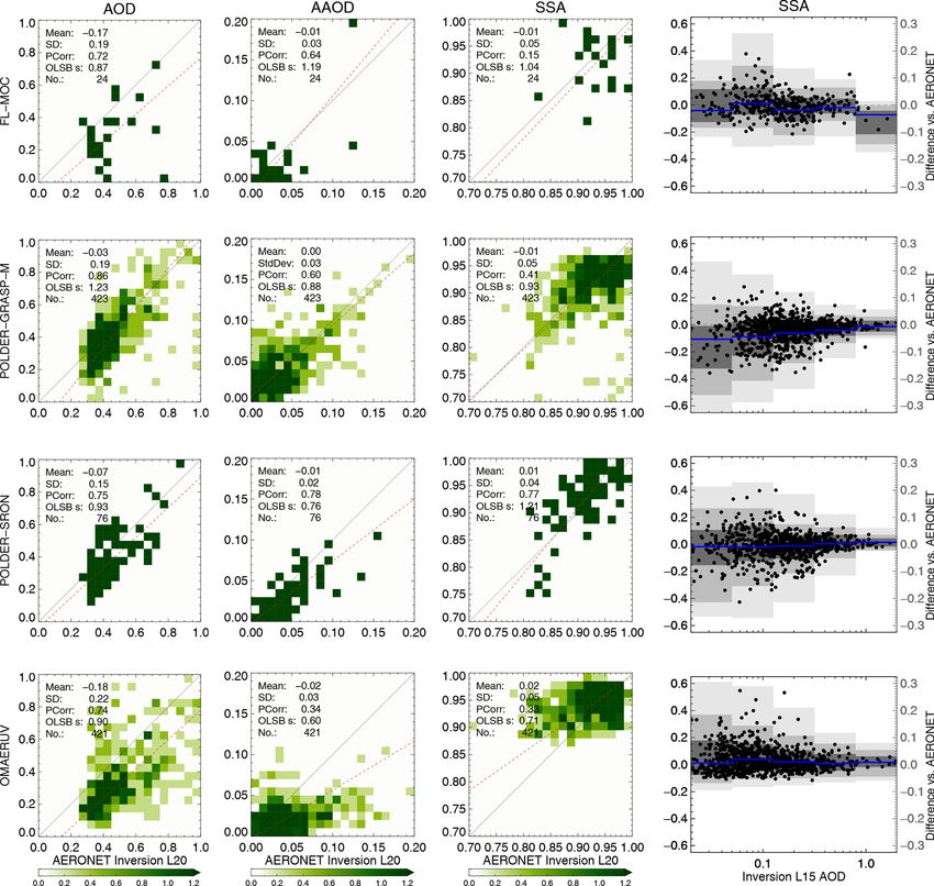
6898                                                     N. Schutgens et al.: AEROCOM and AEROSAT AAOD and SSA study – Part 1

Table 1. Remote sensing products used in this study.

   Platform             Overpass          Sensor               Swath          Pixel   Product      (A)AOD1 Years                   References
                        (h)                                     (km)          (km)                 550 nm
   Aqua/AURA/           01:30PM           MODIS/OMI/CALIOP
                                                         1                       1    FL-MOC1      R             2007, 2008        Kacenelenbogen et al.
   CALIPSO                                                                                                                         (2019)
   AURA                 01:30PM           OMI                    2600           18    OMAERUV      E             2006, 2008,       Ahn et al. (2014),
                                                                                      v1.8.9.1                   2010              Jethva et al. (2014)
   PARASOL              01:30PM2          POLDER                 1600         6.18    POLDER-      I             2006, 2008,       Dubovik et al. (2011),
                                                                                      GRASP-M                    2010              Chen et al. (2020)
                                                                                      v1.2
   PARASOL              01:30PM2          POLDER                 1600         6.18    POLDER-      I             2006              Hasekamp and Landgraf
                                                                                      SRON                                         (2005), Hasekamp et al.
                                                                                                                                   (2011)
 1 This product uses a combination of Aqua-MODIS, OMI and CALIOP observations. 2 PARASOL started drifting away from Aqua at the end of 2009. 3 Interpolated or
 extrapolated to 550 nm, depending on surface type; or retrieved at 550 nm.

mically interpolated or extrapolated from surrounding wave-                              2.1.2   OMAERUV
lengths.
                                                                                         The Ozone Monitoring Instrument (OMI) on the EOS-Aura
2.1.1    FL-MOC                                                                          satellite was deployed in July 2004. It is a high-resolution
                                                                                         spectrograph that measures the upwelling radiance at the top
FL-MOC (Fu–Liou – MODIS, OMI, CALIOP) is a tech-                                         of the atmosphere in the ultraviolet and visible (270–500 nm)
nique for combining CALIOP (Cloud-Aerosol Lidar with                                     regions of the solar spectrum (Levelt et al., 2006). It had
Orthogonal Polarization) aerosol backscatter, MODIS (Mod-                                a 2600 km wide swath and provides daily global coverage
erate Resolution Imaging Spectroradiometer) spectral AOD                                 at a spatial resolution varying from 13 × 24 km at nadir to
and OMI (Ozone Monitoring Instrument) AAOD retrievals                                    28 × 150 km at the extremes of the swath. OMI hyperspec-
for estimating full spectral sets of aerosol radiative proper-                           tral measurements are used as input to inversion algorithms
ties (SSA, asymmetry parameter and AOD). It is not a re-                                 to retrieve ozone vertical distribution and column amounts of
trieval per se but a consistent reinterpretation of the com-                             O3 , NO2 , SO2 , HCHO, BrO and OClO. OMI observations
bined data within their stated uncertainties. Details are given                          are also used to retrieve information on aerosols and clouds.
in Kacenelenbogen et al. (2019, Appendix A). In brief, FL-                                  Aerosol properties in the near UV are derived from OMI
MOC uses the L2 retrieved aerosol properties as input to a                               observations at 354 and 388 nm (Torres et al., 2007). The
simple lookup table retrieval of aerosol types and concentra-                            OMI UV aerosol algorithm (OMAERUV) takes advantage
tions, under the assumption that aerosol properties are con-                             of the large sensitivity to aerosol absorption in the near UV
sistent with the L2 aerosol observations within the stated un-                           discovered in the mid-90s using heritage TOMS instruments
certainties of each sensor’s retrieval. This technique also as-                          (Herman et al., 1997) and the low reflectance of all ice/snow-
sumes that the surface reflectance and clouds are properly                               free terrestrial surfaces, which facilitates the aerosol charac-
treated in the underlying retrievals.                                                    terization over all arid and semi-arid regions of the world.
   Over land, FL-MOC uses OMAERUV (see Sect. 2.1.2)                                      The OMAERUV two-channel algorithm simultaneously re-
AAOD, and over ocean it uses OMAERO AAOD. OMAERO                                         trieves AOD and SSA at 388 nm. The main sources of uncer-
is an advanced multi-wavelength UV–VIS algorithm that                                    tainty are assumed aerosol layer height and cloud contamina-
uses 17 wavelengths in the 331–500 nm range in order to cal-                             tion, with the latter associated with the sensor’s coarse spa-
culate the aerosol optical depth and to discriminate between                             tial resolution. The OMAERUV 15-year record of AOD has
various types of aerosols. It is an extension of the near-UV                             been validated with AERONET observations (Torres et al.,
TOMS (Total Ozone Mapping Spectrometer) method (see                                      2013; Ahn et al., 2014). The SSA record has also been eval-
the OMAERUV product) to a wider wavelength range. The                                    uated by comparisons to AERONET and SKYNET (https:
OMAERO algorithm is applied over all surface types; how-                                 //www.skynet-isdc.org/index.php, last access: 4 May 2021)
ever, its primary objective is to derive aerosol properties over                         ground-based retrievals (Jethva et al., 2014, 2019).
the oceans due to the limited availability of spectral surface
reflectivity databases over land.

Atmos. Chem. Phys., 21, 6895–6917, 2021                                                                     https://doi.org/10.5194/acp-21-6895-2021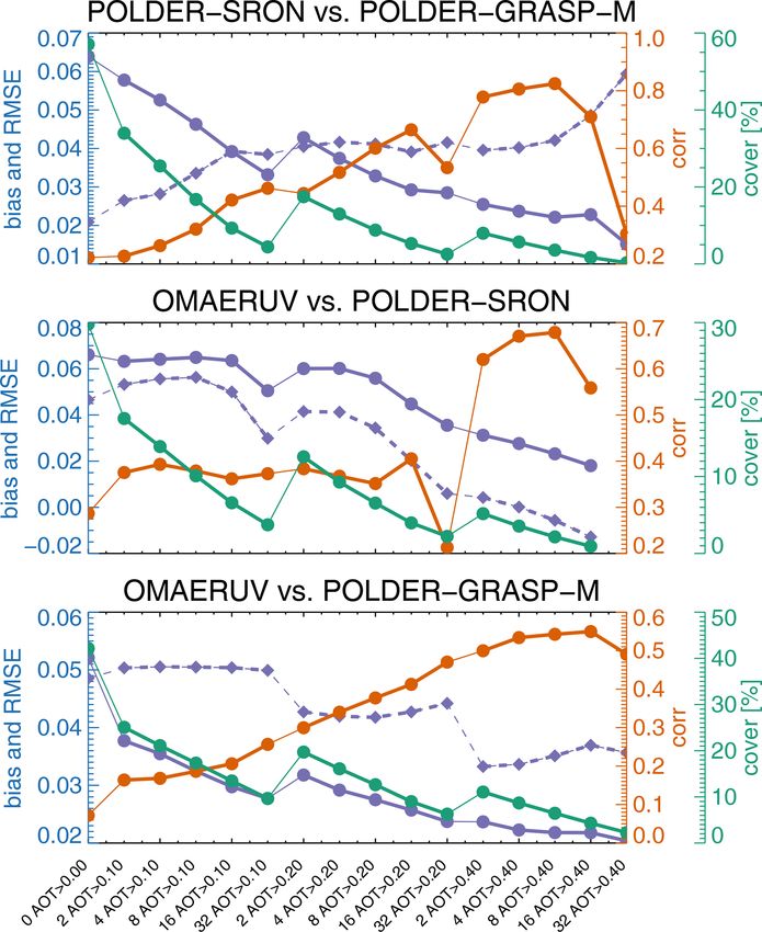
N. Schutgens et al.: AEROCOM and AEROSAT AAOD and SSA study – Part 1                                                         6899

2.1.3   POLDER-SRON                                                 for aerosol–cloud interactions by Hasekamp et al. (2019b),
                                                                    and for data assimilation by Tsikerdekis et al. (2021). Cur-
The POLDER-3 instrument was a multi-angle, multi-                   rently, the algorithm has been applied to 1 year (2006) of
wavelength polarimeter flying aboard the Polarization and           global aerosol data.
Anisotropy of Reflectances for Atmospheric Sciences cou-
pled with Observations from a Lidar (PARASOL) satellite. It         2.1.4   POLDER-GRASP
was launched in 2004 and was a part of the satellite constel-
lation A-Train until 2009. Initially designed to be operated        For a description of the POLDER instrument, see the previ-
for 2 years, POLDER-3 performed its measurements until              ous subsection.
late 2013, when it was decommissioned. PARASOL provides                GRASP (Generalized Retrieval of Aerosol and Sur-
measurements of a ground scene under (up to) 16 different           face Properties) is a unified retrieval algorithm for atmo-
viewing geometries in 9 spectral bands (443, 490, 565, 670,         sphere properties from diverse remote sensing observations
763, 765, 865, 910, 1020 nm). Linear polarization measure-          (Dubovik et al., 2011, 2014), based on earlier work by
ments (Stokes parameters Q and U ) are performed in three           Dubovik and King (2000), and Dubovik et al. (2002) and
spectral bands (490, 670, 865 nm). Its spatial resolution at the    Dubovik et al. (2006) for AERONET inversions.
nadir was about 6 km, and its swath width was 2400 km.                 In the current paper, retrievals from the so-called “mod-
   An advanced retrieval algorithm making full use of the in-       els” dataset are used. Aerosol is assumed to be an external
formation content of the multi-angle photopolarimetric ob-          mixture of five different aerosol components which are re-
servations from POLDER-3/PARASOL has been developed                 trieved together with spectral parameters of surface BRDF
at SRON (Netherlands Institute for Space Research). The al-         and BPDF (bidirectional polarization distribution function).
gorithm has large flexibility in defining the aerosol proper-       The aerosol is assumed to be a mixture of spherical and non-
ties included in the retrieval state vector (Fu and Hasekamp,       spherical particles. Each fraction is characterized by particle
2018). The aerosol size distribution is described by the            size distributions similarly to AERONET retrievals. The non-
sum of an arbitrary number of log-normal functions, called          spherical component is modelled as a mixture of randomly
modes, where for each mode the effective radius (reff ), effec-     oriented spheroids with fixed shape distribution (Dubovik
tive variance (veff ), aerosol column number, real and imagi-       et al., 2006). The details of the “models” approach are dis-
nary parts of the refractive index (in the form of coefficients     cussed by Lopatin et al. (2021) and Chen et al. (2020).The
of spectrally dependent functions), fraction of spherical parti-    actual inversion uses multi-pixel retrieval (Dubovik et al.,
cles assuming the mixture of spheres and spheroids proposed         2011) where horizontal pixel-to-pixel variations of aerosol
by Dubovik et al. (2006), and the aerosol layer height can (in      and day-to-day variations of surface reflectance are enforced
principle) be retrieved. In the setup used in the present study,    to be smooth.
the POLDER-SRON algorithm yields the different micro-                  The full archive of POLDER/PARASOL observations was
physical characteristics of a bimodal aerosol size distribution     retrieved using GRASP and can be found at https://www.
(fine and coarse mode), with the fraction of spheres only be        grasp-open.com (last access: 4 May 2021). In addition to
retrieved for the coarse mode (fine mode assumed to consist         the “models” dataset, two other datasets are available (“op-
only of spheres) and the aerosol layer height fixed to 1 km.        timized” and “high-precision”) that use slightly different as-
For retrievals over ocean, the state vector also includes the       sumptions in the retrieval. The detailed discussion and vali-
wind speed, chlorophyll a concentration and whitecap frac-          dation of all three 0.1◦ PARASOL/GRASP retrievals are pro-
tion, while for retrievals over land, the state vector includes     vided by Chen et al. (2020). The “models” dataset used in
the parameters describing the surface BRDF (bidirectional           this paper is considered the most applicable for a wide range
reflectance distribution function) (Litvinov et al., 2011). The     of circumstances.
retrieval is based on an iterative fitting of a linearized radia-      The dataset used in the current paper is aggregated
tive transfer model (Hasekamp and Landgraf, 2005) to the            to 1◦ spatial resolution (details are listed at https://www.
PARASOL data, using a cost function containing a misfit             grasp-open.com). The “models” dataset provides AOD and
term between the forward model and measurement and a reg-           AAOD aggregated from slightly different L2 samplings: an
ularization term using a priori estimates of values of some of      additional minimum AOD threshold is used when aggregat-
the retrieved parameters. The algorithm, including an appli-        ing AAOD. To select data of higher quality, AAOD retrievals
cation to PARASOL measurements over ocean, is described             were used only for cases with sufficient aerosol loading. The
in Hasekamp et al. (2011). More recent refinements are de-          same AOD threshold is used for SSA as well. Specifically,
scribed by Stap et al. (2015), Wu et al. (2015), Lacagnina          minimum AOD (at 440 nm) thresholds of 0.3 over land and
et al. (2015), Fu and Hasekamp (2018), and Fu et al. (2020).        0.02 over ocean were applied (the threshold over ocean is
Retrieval results from the SRON algorithm have been used            probably too low to assure high-quality AAOD, but higher
for aerosol type determination by Russell et al. (2014), in         thresholds result in significant data loss).
studies related to aerosol absorption and direct radiative ef-         In the current study we prefer to use aggregated AOD and
fect by Lacagnina et al. (2015) and Lacagnina et al. (2017),        AAOD data that describe the exact same scene, and this is

https://doi.org/10.5194/acp-21-6895-2021                                             Atmos. Chem. Phys., 21, 6895–6917, 2021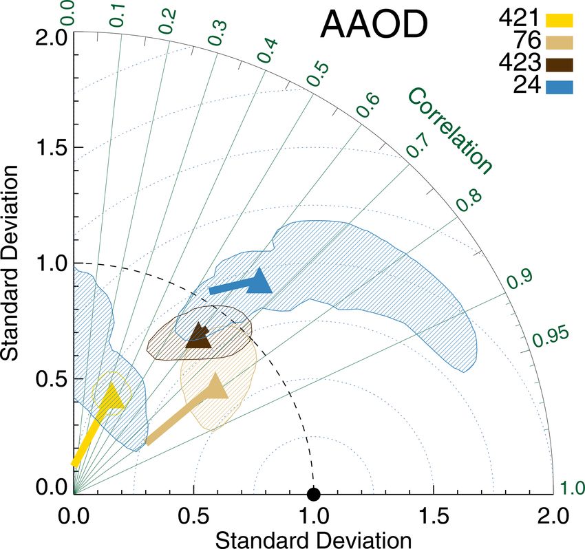
6900                                     N. Schutgens et al.: AEROCOM and AEROSAT AAOD and SSA study – Part 1

the case for the FL-MOC, OMAERUV and POLDER-SRON                (or, for that matter, AAOD) datasets is that there is no estab-
datasets mentioned earlier. For the GRASP product, we de-       lished gold standard.
cided to assume that the aggregated SSA represents the same        The Inversion dataset also contains AOD (from DirectSun
scene as the AOD aggregate and recalculated an AAOD from        retrievals) which is actually used in the inversion. Here we
that AOD and SSA. Consequently, the AAOD product (in-           only use those AOD values in the Inversion dataset that have
dicated as GRASP-M) presented in this paper is different        corresponding AAOD and SSA values, so that aggregate val-
from the AAOD found in the official L3 “models” product. In     ues always describe the same scene.
situ measurements (Delene and Ogren, 2002; Andrews et al.,         Inversion L2.0 is a subset of L1.5 (which contains almost
2011, 2017; Schmeisser et al., 2018) have suggested a change    30 times more observations), based on further cloud screen-
in SSA at lower AOD, so our SSA assumption may intro-           ing and the requirement that AOD at 440 nm ≥ 0.4. This last
duce additional biases. However, GRASP-M AAOD evalu-            criterion results in a minimum AOD at 550 nm of 0.25 in the
ated better against AERONET than “models” AAOD which            Inversion L2.0 product.
showed a high bias vs. AERONET due to the aforementioned           Since an individual AERONET site is not necessarily rep-
minimum AOD threshold.                                          resentative of a 1◦ × 1◦ grid box, satellite evaluation may
   For this study the L3 GRASP data were additionally fil-      be negatively affected. To select only sites with high repre-
tered based on the fitting residual field, which was required   sentativity, we use a list published in Kinne et al. (2013) as
to be smaller than 0.05 (over land) or 0.1 (over ocean). This   described in Schutgens et al. (2020), where we also tested
subset evaluates substantially better for AOD retrievals and    this representativity (using 14 satellite AOD products). The
somewhat better for AAOD retrievals than the full dataset.      Kinne list was developed with the AERONET DirectSun
                                                                product (i.e. AOD) in mind, but a high-resolution modelling
                                                                study by Schutgens (2020) suggests that spatial representa-
2.1.5   AERONET
                                                                tivity for AOD and AAOD observations can differ substan-
                                                                tially for individual sites. We chose to use the Kinne list be-
AERONET (Holben et al., 1998) DirectSun V3 L2.0 (Giles          cause it also includes information on maintenance quality,
et al., 2019; Smirnov et al., 2000) and Inversion V3 L1.5 and   likely more important for Inversion than DirectSun retrievals.
2.0 data were downloaded from https://aeronet.gsfc.nasa.gov
(last access: 4 May 2021), logarithmically interpolated to      2.1.6   How independent are these satellite products?
values at 550 nm and aggregated by averaging over 30 min.
The DirectSun dataset contains only AOD (at multiple wave-      An interesting question is how independent these satellite
lengths). These observations are based on direct transmission   products are.
measurements of solar light and have a low uncertainty of          The GRASP and SRON algorithms are independent re-
±0.01 (Eck et al., 1999; Schmid et al., 1999), at 400 nm and    trieval codes with many specific differences in the implemen-
larger.                                                         tation. First, in the present study POLDER-SRON retrieves
   The Inversion dataset contains AAOD and SSA (at multi-       parameters of bimodal lognormal size distribution and com-
ple wavelengths) based on measurements of scattered solar       plex refractive index for each size mode, while POLDER-
light from multiple directions. This inversion uses radiative   GRASP-M retrieves the concentrations of five aerosol com-
transfer calculations (Dubovik and King, 2000) and yields       ponents with assumed properties of each component (Chen
larger errors than the DirectSun measurements. In particu-      et al., 2020; Lopatin et al., 2021). Second, GRASP and
lar, Dubovik et al. (2000) showed that SSA errors decrease      SRON use the same mathematical function for the BRDF
with increasing AOD and estimated 440 nm SSA errors of          over land (Litvinov et al., 2011) but estimate the parameters
±0.03 for water-soluble aerosol at 440 nm AOD ≥ 0.2, al-        to this function independently. In both algorithms, aerosol
though for dust and biomass burning aerosol higher AOD          and surface properties are estimated simultaneously. Third,
values ≥ 0.5 were needed. These error estimates were based      there are significant differences in the use of a priori con-
on numerical calculations. A recent in-depth estimate of the    straints. POLDER-SRON follows Phillips–Tikhonov regu-
uncertainty in Inversion V3 data (Sinyuk et al., 2020) sug-     larization (Phillips, 1962; Tikhonov, 1963) including a priori
gested those thresholds to be 440 nm AOD > 0.3 and ≥ 0.45,      estimates for most of the retrieved state vector parameters (a
respectively. For an examination of the impact of geomet-       globally constant value is used) and a flexible strength of the
rical configuration on SSA observations, see Torres et al.      regularization term. The GRASP algorithm is based on the
(2014). Schafer et al. (2014) showed that AERONET SSA           least squares multi-term approach (see Dubovik et al., 2011)
retrievals were lower by 0.011 than flight campaign data (on    and uses several a priori constraints simultaneously. Specifi-
average). Andrews et al. (2017) also compared flight cam-       cally, GRASP “models” uses smoothness constraints on the
paign measurements to AERONET SSA and found that the            spectral dependence of surface BRDF parameters. Fourth,
data were usually within the expected errors, although at low   the SRON algorithm retrieves from measurements of indi-
AOD ≤ 0.2 significantly lower SSA values were observed by       vidual pixels, while the GRASP algorithm retrieves from
AERONET. A confounding issue for the evaluation of SSA          measurements of multiple pixels simultaneously, applying

Atmos. Chem. Phys., 21, 6895–6917, 2021                                          https://doi.org/10.5194/acp-21-6895-2021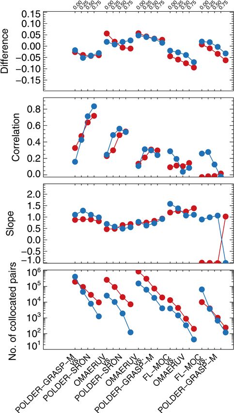
N. Schutgens et al.: AEROCOM and AEROSAT AAOD and SSA study – Part 1                                                               6901

spatio-temporal constraints in the process. For example, over
land constraints were used to limit the temporal variability of
retrieved BRDF parameters as well as the spatial variability
of aerosol retrieved parameters (see Dubovik et al., 2011, and
Chen et al., 2020).
   The FL-MOC product uses OMAERUV AAOD as input
over land, but FL-MOC only uses OMAERUV AAOD as
an a priori estimate and assigns this a sizeable uncertainty.
CALIOP backscatter is expected to provide a constraint on
SSA and consequently AAOD. As a matter of fact, our anal-          Figure 2. Correlation of satellite AOD (solid) and AAOD (dashed)
ysis shows that FL-MOC and OMAERUV exhibit rather low              with AERONET Inversion L2.0 data, as a function of a tempo-
correlations for AAOD (and SSA). This suggests that the            ral collocation criterion. Colours indicate the satellite product (see
OMAERUV a priori estimate does not lead to a strong de-            also Fig. 1). Satellite products were individually collocated with
pendency of FL-MOC on OMAERUV. On the other hand,                  AERONET.
it also suggests that at least one of these products contains
sizeable errors.                                                   ways derived from averaged AOD and AAOD:

                                                                   SSA = 1 − AAOD/AOD.                                               (1)
3   Collocation and analysis methodology
                                                                      During the evaluation of products with AERONET, a dis-
To evaluate and intercompare the remote sensing datasets,          tinction will be made between either land or ocean grid boxes
they will need to be collocated in time and space to reduce        in the common grid. A high-resolution land mask was used
representation errors (Colarco et al., 2014; Schutgens et al.,     to determine which 1◦ × 1◦ grid box contained at most 30 %
2016a, 2017). In practice this collocation is another aggre-       land (designated an ocean box) or water (designated a land
gation (performed for each dataset individually) to a spatio-      box). Most ocean boxes with AERONET observations will
temporal grid with slightly coarser temporal resolution (1 or      be in coastal regions, with some over isolated islands.
3 h; the spatial grid box size remains 1◦ × 1◦ ). This is fol-
                                                                   3.1   Taylor diagrams
lowed by a masking operation that retains only aggregated
data if they exist in the same grid boxes for all involved         A suitable graphic for displaying multiple datasets’ corre-
datasets. More details can be found in Appendix A.                 spondence with a reference dataset (truth) is provided by
   We need to allow some flexibility in the time separation        the Taylor diagram (Taylor, 2001). In this polar plot, each
between data (here 3 h) to ensure sufficient numbers of col-       data point (r, φ) shows basic statistical metrics for an en-
located data pairs for further analysis. Schutgens et al. (2020)   tire dataset. The distance from the origin (r) represents the
showed that shorter time separations greatly limited the num-      internal variability (standard deviation) in the dataset. The
ber of pairs but did not substantially alter the correlation of    angle φ through which the data point is rotated away from
satellite AOD with AERONET. On the other hand, longer              the horizontal axis represents the correlation with the refer-
time separations appear to negatively affect the correlation       ence dataset, which is conceptually located on the horizontal
of satellite AAOD with AERONET (see Fig. 2). The analysis          axis at radius 1 (i.e. every distance is normalized to the in-
shows that satellite AOD correlation with AERONET Inver-           ternal variability of the reference dataset). It can be shown
sion data slowly decreases as the collocation criterion is re-     (Taylor, 2001) that the distance between the point (r, φ) and
laxed from 3 to 24 h. However, satellite AAOD shows a sharp        this reference data point at (1, 0) is a measure of the root
drop in correlation with AERONET at 6 h (OMAERUV is the            mean square error (RMSE, unbiased). A line extending from
exception; the correlation is already low and barely changes).     the point (r, φ) is used to show the bias versus the reference
We surmise this is due to plumes of absorbing aerosol drift-       dataset (positive for pointing clockwise). The distance from
ing over the sites, requiring tight temporal constraints on col-   the end of this line to the reference data point is a measure
location. Consequences of this finding will be further dis-        of the root mean square difference (RMSD, no correction for
cussed in Sect. 7.                                                 bias).
   As the FL-MOC dataset, based on CALIOP measure-
ments, is smaller than the other satellite datasets, we were       3.2   Uncertainty analysis using bootstrapping
compelled to collocate FL-MOC with AERONET within 2◦
instead of 1◦ . Even so, the data count for the FL-MOC eval-       Our estimates of error metrics are inherently uncertain due
uation is low.                                                     to finite sampling. If the sampled error distribution is suffi-
   After spatio-temporally collocating two or more datasets,       ciently similar to the underlying true error distribution, boot-
the data may be further averaged in space and/or time for          strapping (Efron, 1979) can be used to assess uncertainties
analysis purposes. Spatio-temporally averaged SSA is al-           in for example biases or correlations due to finite sample

https://doi.org/10.5194/acp-21-6895-2021                                             Atmos. Chem. Phys., 21, 6895–6917, 2021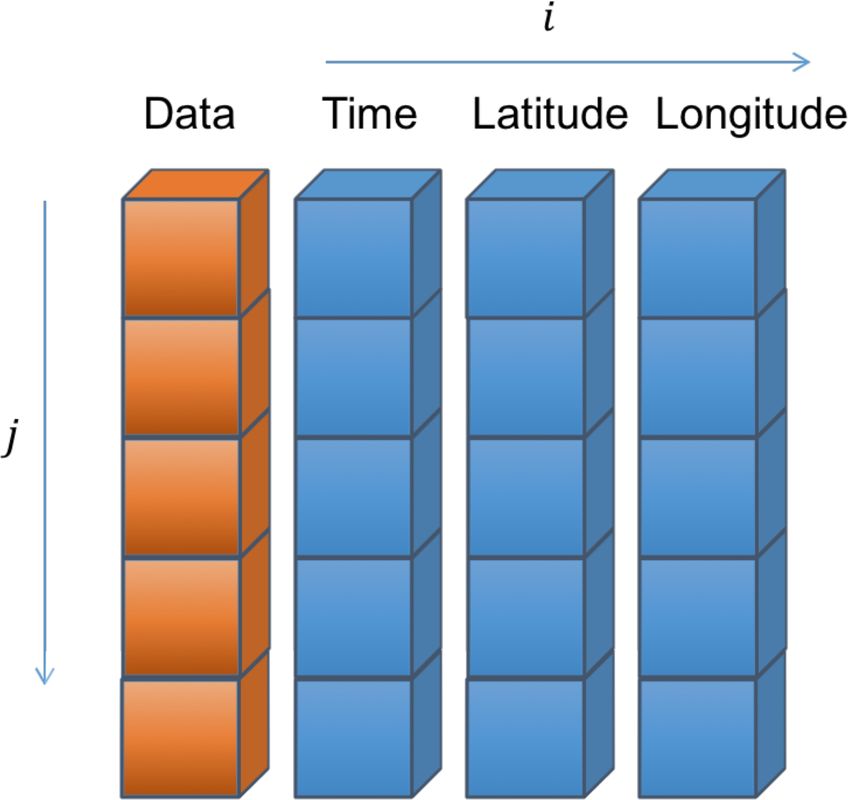
6902 N. Schutgens et al.: AEROCOM and AEROSAT AAOD and SSA study – Part 1
size. Bootstrapping uses the sampled distribution to generate
a large number of synthetic samples by random draws with
replacement. For each of these synthetic samples, a bias can
be calculated, and the distribution of these biases provides
measures of the uncertainty, e.g. a standard deviation, in the
bias due to statistical noise. Bootstrapping has been shown
to be reliable even for relatively small sample sizes (that is,
the size of the original sample and not the number of boot-
straps; see Chernick, 2008). In this study, the uncertainty bars
in some figures were generated by bootstrap analysis.
If the sampled error distribution is different from the true
error distribution, bootstrapping will likely underestimate
uncertainties. Sampled error distributions may be different
from the true error distribution because the act of collocat-
ing satellite and AERONET data favours certain conditions. Figure 3. Global biases in four satellite AOD datasets depending on
the chosen reference dataset (DirectSun or Inversion). Colours indi-
For example, the effective combination of two cloud screen-
cate the satellite product (see also Fig. 1). Numbers in upper left and
ing algorithms (one for the satellite product and the other for lower right corner indicate the amount of collocated data, averaged
AERONET) may favour clear-sky conditions and reduce our over all products. Error bars indicate a 5 %–95 % uncertainty range
sampling of errors due to cloud contamination. This uncer- based on a bootstrap analysis (see Sect. 3.2). Satellite products were
tainty due to sampling is unfortunately hard to assess (see individually collocated with AERONET within 3 h.
e.g. Schutgens et al., 2020).
As an example of uncertainty due to sampling, we present
Fig. 3, in which an evaluation of the current satellite AOD are based on collocated data and confirm major features. The
data with Inversion L2.0 data (only those AOD values products all agree on a major AAOD hotspot (likely) from
that have corresponding AAOD inversions, which constrains the African savannah biomass burning. Three products agree
AOD at 440 nm > 0.4) shows substantial shifts compared on AAOD hotspots in China and India, which are known pol-
to DirectSun L2.0. As the uncertainty ranges indicate, the luted regions. (OMAERUV, which is relatively featureless, is
changes in biases are not due to statistical noise. Neither is the exception. We surmise this is due to the large pixel size
this due to differences in collocated DirectSun and Inver- of the OMI instrument (see Table 1), which will not resolve
sion L2.0 AOD values, which agree very well. Rather, the small-scale structure in AAOD. The existence of such small-
issue is that AERONET Inversion data are an unrepresen- scale structure was inferred from Fig. 2.) POLDER-GRASP-
tative subsample of the DirectSun data (Inversion data are M and OMAERUV show a clear AAOD hotspot due to Ama-
skewed to high AOD). It is unclear what this means for the zonian biomass burning. POLDER-GRASP-M estimates rel-
AAOD and SSA evaluation, but readers should be aware of atively high values over land and the ocean at high northern
this unaccounted-for sampling issue that may introduce bi- latitudes. OMAERUV shows relatively low AAOD over land
ases. but high over the entire ocean. FL-MOC clearly estimates
higher AAOD over the Sahara than either POLDER-GRASP-
3.3 Error metrics for evaluation M or OMAERUV. POLDER-SRON estimates relatively high
AAOD over the Rocky Mountains, the Andes and Australia.
We will use the usual global error statistics (bias, standard Unfortunately, even in multi-year averages significant differ-
deviation, Pearson correlation, regression slopes), treating all ences in regional AAOD between the products are observed,
data as independent. Regression slopes were calculated with in excess of 50 %. Figure S1 in the Supplement shows the
a robust ordinary least squares regressor (OLS bisector from corresponding SSA maps. As expected, POLDER-GRASP-
the IDL sixlin function, Isobe et al., 1990). This regres- M has relatively low SSA and OMAERUV relatively high
sor is recommended when there is no proper understanding SSA over land. FL-MOC has the highest SSA over ocean of
of the errors in the independent variable (see also Pitkänen all products. As the satellite AOD values are fairly similar,
et al., 2016). lower values of AAOD translate into higher values of SSA.
One caveat is that AAOD and SSA retrievals are likely to
be better (more accurate and precise) at high AOD. In the
4 A first look at the satellite products above analysis, no account was taken of AOD levels, and
the products were discussed as they are. The impact of AOD
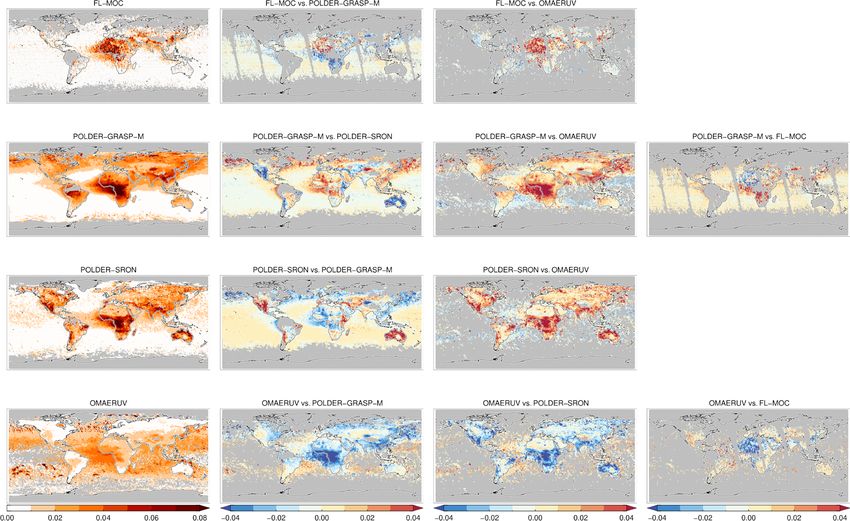
Multi-year averages of satellite AAOD and their differences will be discussed later, when discussing the evaluation with
are shown in Fig. 4. The AAOD maps can only be compared AERONET in Sect. 5.2 and the satellite intercomparison in
with caution, as they are derived from products with differ- Sect. 6.
ent temporal sampling. The differences, on the other hand,
Atmos. Chem. Phys., 21, 6895–6917, 2021 https://doi.org/10.5194/acp-21-6895-2021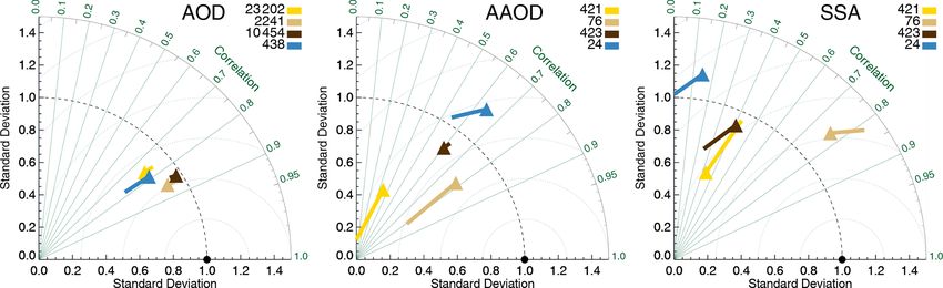
N. Schutgens et al.: AEROCOM and AEROSAT AAOD and SSA study – Part 1                                                             6903

Figure 4. Global maps of AAOD for four products and their differences. AAOD differences are based on collocated data (within 3 h). Note
that the products are available for different years; e.g. POLDER-SRON and FL-MOC do not overlap. No minimum AOD was required.

5   Evaluation of satellite products with AERONET                        The impact of statistical noise on the AAOD evaluation
                                                                      is explored in Fig. 6. Using a bootstrapping technique, the
Taylor plots of the performance of the satellite products             spread in correlation and standard deviation were explored.
are shown in Fig. 5. Satellite AOD is evaluated against               For most datasets, the results seem fairly robust, except for
AERONET DirectSun L2.0. Satellite AAOD and SSA are                    FL-MOC, which yielded only 24 data points. A proper inter-
evaluated against AERONET Inversion L2.0 (which con-                  comparison of products requires collocation (of all the satel-
strains AOD at 440 nm > 0.4 and provides much less data               lite data), which reduces available cases even further. Fig-
than DirectSun). All products show high correlation with              ure S2 shows that results are not very different from Fig. 5,
AERONET AOD (r ≥ 0.76), although the correlations found               but the statistical noise increases substantially. The sampling
are lower than those found in Schutgens et al. (2020) for             noise on such a small subset should be even larger (see also
several MODIS Aqua products (0.87–0.88). Correlations for             Fig. 3 and Schutgens et al., 2020). For a sense of perspec-
AAOD and SSA are lower than for AOD, suggesting that it               tive, 48 data points represents less than 0.0008 % of the total
is more challenging to retrieve absorbing qualities.                  POLDER-GRASP-M data amount used in this paper.
   Interestingly, POLDER-SRON’s SSA correlates signifi-
cantly better with AERONET than POLDER-GRASP-M’s                      5.1   Evaluation and intercomparison of AOD
SSA, but this is a sampling effect: once both products
are collocated together, POLDER-GRASP-M’s SSA corre-                  In Fig. 7, we provide more detail on the satellite AOD prod-
lation with AERONET increases from 0.41 to 0.69. The                  ucts and their evaluation against AERONET DirectSun L2.0
explanation for this is not entirely clear, although it turns         AOD. In the central column, we show the products them-
out that POLDER-GRASP-M evaluates more poorly with                    selves, averaged over 1, 2 or 3 year(s), depending on avail-
AERONET for 2010 than for 2006 and 2008 (POLDER-                      ability (see Table 1). Note that the products exist for different
SRON is currently limited to 2006; see Table 2.1). Although           years, and even for the same years products will have differ-
the poorer evaluation for 2010 can be seen in AOD, AAOD               ent temporal samplings, so comparisons should be made with
and SSA, it is only statistically significant for SSA.                caution (Colarco et al., 2014; Schutgens et al., 2016a). In the
                                                                      left and right column, we show satellite data collocated with

https://doi.org/10.5194/acp-21-6895-2021                                               Atmos. Chem. Phys., 21, 6895–6917, 2021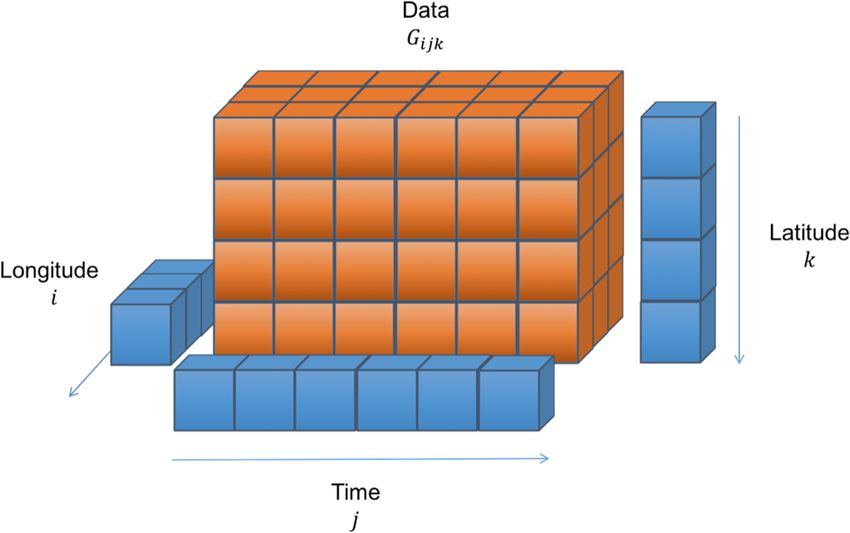
6904                                           N. Schutgens et al.: AEROCOM and AEROSAT AAOD and SSA study – Part 1

Figure 5. Taylor diagrams (for an explanation, see Sect. 3.1) for the satellite products. AOD is evaluated against AERONET DirectSun L2.0,
and AAOD and SSA are evaluated against AERONET Inversion L2.0. Colours indicate the satellite product (see also Fig. 1), and numbers
next to coloured blocks indicate the amount of collocated data. The lines extending from the data points indicate the bias. Products were
individually collocated with AERONET within 3 h.

                                                                        OMAERUV overestimates everywhere except in some re-
                                                                        gions with strongly absorbing aerosol. An intercomparison
                                                                        of satellite AOD with Aqua-DT (Dark Target) is presented in
                                                                        Fig. S3 and suggests typically higher estimates over (South-
                                                                        ern Hemisphere) land for the POLDER products and over
                                                                        ocean for OMAERUV. Note that Aqua-DT is not without sig-
                                                                        nificant regional biases (see Schutgens et al., 2020).
                                                                           Figure 8 shows results when bias (signless) and correlation
                                                                        per site (that yielded at least 32 collocations) are averaged
                                                                        over all sites for each satellite product. The same 52 sites
                                                                        are used for all datasets, although each product is individu-
                                                                        ally collocated with AERONET. For FL-MOC, no site pro-
                                                                        vided at least 32 observations, and this is not included in the
Figure 6. Impact of statistical noise on the correlation and internal   analysis. For POLDER-SRON, only 18 sites provided at least
variability of satellite AAOD products, using bootstrapping. Shaded     32 collocated observations, and this was similarly excluded.
regions indicate a 5 %–95 % uncertainty range of correlation and        As was also shown in Schutgens et al. (2020), OMAERUV
standard deviation (uncertainty in bias is not shown). Colours in-      shows rather large biases compared to the other AOD prod-
dicate the satellite product (see also Fig. 1), and numbers next to     ucts. POLDER-GRASP-M, on the other hand, shows the
coloured blocks indicate the amount of collocated data. Satellite       smallest bias. The filtering of GRASP retrievals described
products were individually collocated with AERONET Inversion            in Sect. 2.1 plays a significant role in this result (without fil-
L2.0 within 3 h.                                                        tering, POLDER-GRASP-M shows a bias twice as large).

                                                                        5.2   Evaluation of AAOD and SSA
AERONET. On the left-hand side is a scatter plot of the data
(with associated statistics provided), and on the right-hand            Figure 9 provides more detail on the evaluation of satel-
side is a map of multi-year difference with AERONET (pro-               lite (A)AOD and SSA products against AERONET Inversion
vided at least 32 data points were available per site).                 L2.0 (which constrain AOD at 440 nm > 0.4). In the first
   The scatter plots show good correlation with AERONET.                three columns, we show scatter plots for respectively AOD,
The POLDER products show higher correlations and slopes                 AAOD and SSA. In the last column we show SSA differ-
closer to one (1) than FL-MOC and OMAERUV. Never-                       ences with AERONET as a function of AERONET AOD (In-
theless, differences in evaluation seem rather small, which             version L1.5). All products underestimate AERONET AOD
unfortunately cannot be said for the global distributions               and AAOD, although only by a small amount in the case
of AOD. POLDER-GRASP-M has rather high AOD over                         of POLDER-GRASP-M. More importantly, AAOD correla-
land, and OMAERUV has rather high AOD over ocean                        tions can be as low as 0.34 (OMAERUV), and the regression
(note that the satellite data themselves are not collocated).           slope can deviate substantially from 1 (0.6 for OMAERUV).
The multi-year differences with AERONET suggest that                    In contrast, some products underestimate SSA, while oth-

Atmos. Chem. Phys., 21, 6895–6917, 2021                                                   https://doi.org/10.5194/acp-21-6895-2021
N. Schutgens et al.: AEROCOM and AEROSAT AAOD and SSA study – Part 1 6905
Figure 7. For the four satellite products the following are shown: a scatter plot of individual super-observations versus AERONET (the
colour indicates amount of data in percentages; see Sect. 3.3 for an explanation of the metrics), a global map of the 3-year AOD average and
a global map of the 3-year AOD difference average with AERONET (if the site provided at least 32 observations; land sites are circles, ocean
sites are squares, and diamonds are the remainder). For FL-MOC, insufficient data prevent the plotting of a difference map. Products were
individually collocated with AERONET DirectSun L2.0 within 3 h.
ers overestimate it. Due to data sparsity (e.g. for POLDER- The rightmost column in Fig. 9 shows the SSA difference
GRASP-M, the count dropped from 10 454 to 423), it is not as a function of (AERONET) AOD. To ensure the largest
possible to do an analysis for each AERONET site (as was possible range in AOD values, Inversion L1.5 instead of L2.0
done for AOD) and see how the global bias relates to re- is used. Especially at lower AOD, this dataset will have larger
gional biases. The bootstrap analysis suggest that results are errors in AAOD and SSA than L2.0. Interestingly, as AOD
fairly robust against statistical noise (except FL-MOC; see increases, all satellite products seem to agree better with
also Fig. 6). AERONET (for FL-MOC, the bin with largest AOD val-
ues is affected by a very low data count). This is of course
https://doi.org/10.5194/acp-21-6895-2021 Atmos. Chem. Phys., 21, 6895–6917, 20216906 N. Schutgens et al.: AEROCOM and AEROSAT AAOD and SSA study – Part 1
A profound problem is the paucity of data. Even for
POLDER-GRASP-M, we can only evaluate its performance
(against AERONET) for less than 0.006 % of the total num-
ber of available observations. Is this sufficient to make mean-
ingful statements about the performance of a product at
large? In Schutgens et al. (2020), we showed that the pro-
cess of collocation can skew error statistics (by changing the
sampling) to the point that it becomes hard to meaningfully
distinguish the performance of several products. That study
was done for AOD, which allows much higher numbers of
collocated data with AERONET than AAOD.
To elucidate this, we compare the difference in SSA be-
Figure 8. Evaluation of satellite products with AERONET per site, tween the two POLDER products (collocated within 3 h, con-
averaged over all sites. Squares indicate products used in the present
sidering AOD ≥ 0.25 only) for three different samplings.
study, and circles indicate products used in Schutgens et al. (2020).
Error bars indicate a 5 %–95 % uncertainty range based on a boot-
First, we look at global POLDER SSA statistics. Secondly,
strap analysis (see Sect. 3.2) of sample size 1000 (the bootstrap was we look at POLDER SSA statistics over AERONET sites
performed on the contributing AERONET sites). Colours indicate only. Thirdly, we look at POLDER SSA statistics that are
the satellite product (see also Fig. 1). Products were individually collocated with AERONET observations. Figure 10 shows
collocated with AERONET DirectSun L2.0 within 3 h. All products the associated difference distributions. Using various non-
use the same sites, each of which produced at least 32 collocations. parametric statistical tests (Mann–Whitney U, Student’s t,
POLDER-SRON and FL-MOC were excluded from this analysis Kolmogorov–Smirnov), we can show that the distribution
due to lack of data. means for the first and third sampling are significantly dif-
ferent. Not only that, but the mean difference in SSA for the
first sampling is 2.6 times as large (−0.043 vs. −0.017) as
as one would expect. For smaller AOD, there is increas-
for the third sampling. As POLDER-SRON is biased high
ingly more spread, although the difference distribution re-
and POLDER-GRASP-M is biased low vs. AERONET, the
mains fairly unbiased. The exception is POLDER-GRASP-
corollary to this is of course that at least one of the products
M, which shows increasingly lower SSA than AERONET at
has a larger bias vs. the truth globally than can be seen in the
low AOD. We suggest that it is rather unlikely that three dif-
AERONET observations. Conversely this suggests that the
ferent satellite products have an SSA bias at low AOD that
AERONET Inversion dataset does not allow a truly global
is similar to AERONET (and hence show no bias in the dif-
evaluation of satellite datasets: it provides a subsample with
ference with AERONET) and that this low bias in POLDER-
skewed statistics of SSA errors. Incidentally, it is the tempo-
GRASP-M analysis is real. However, a better understanding
ral subsampling enforced by collocation with AERONET ob-
of the nature of errors (bias vs. random) in AERONET SSA
servations that causes the largest shift in the difference distri-
at low AOD is desirable.
bution (POLDER measurements over AERONET sites show
Summarizing, there is skill in satellite AAOD and SSA,
an SSA distribution similar to the global dataset). It is possi-
but compared to AOD the correlations with AERONET are
ble that the SSA difference is partly driven by cloud contam-
substantially lower. POLDER-SRON is the exception, with
ination, which we know is present in these satellite datasets
similar and fairly high correlations (∼ 0.75) for all three
(Schutgens et al., 2020), and may be ameliorated when a
parameters. However, it seems to underestimate AAOD by
third cloud masking (from AERONET) is applied (through
∼ 25 % at high AAOD (slope of 0.76 in the AAOD scat-
the collocation of data).
ter plot). OMAERUV appears to show the largest deviations
from AERONET (low correlations and slopes), but its overall
error statistics (mean and standard deviation) is not too dif- 6 Intercomparison of satellite AAOD and SSA
ferent from the other products. Results for FL-MOC may be a
statistical fluke due to the low data count. POLDER-GRASP- To get a better appreciation of the satellite products, we now
M shows quite high correlations for AOD (0.86) and AAOD present a global intercomparison. To start with, Fig. 11 shows
(0.6) with reasonable slopes but has a very low correlation SSA differences between two products as a function of their
with AERONET for SSA (0.41), but this seems to depend mean AOD. As in Fig. 9, these differences become smaller
strongly on sampling as discussed at the start of this section. (i.e. show a smaller spread) at higher AOD, as expected (in-
In addition, it appears to systematically underestimate SSA tercomparisons with FL-MOC are the exception). However,
at low AOD. Yet another aspect to this dataset (not visible in satellite SSA values still exhibit random differences of 0.03
any of the analysis shown) is that it appears to have a hard or larger for AOD '1, as also confirmed by the AERONET
SSA cut-off as SSA values larger than 0.99 do not occur. evaluation. In addition, substantial biases remain.
Atmos. Chem. Phys., 21, 6895–6917, 2021 https://doi.org/10.5194/acp-21-6895-2021N. Schutgens et al.: AEROCOM and AEROSAT AAOD and SSA study – Part 1 6907 Figure 9. Evaluation of super-observations of AOD, AAOD and SSA for the satellite products. SSA is also evaluated as a function of AOD (binned). In the three leftmost figures, the colour indicates amount of data in percentages; for an explanation of the metrics, see Sect. 3.3. The rightmost column uses two vertical axes: the left y axis is used for individual data points (subsampled), and the right y axis is used for the greyscale distribution (9 %, 25 %, 50 %, 75 % and 91 % quantiles of the differences) and the median difference (blue line). Products were individually collocated with AERONET Inversion L2.0 within 3 h, except for the rightmost column, which used Inversion L1.5. The previous analysis was global, but substantial differ- fairly constant (POLDER products), decrease (OMAERUV ences can be seen between land and ocean scenes. For in- vs. POLDER-GRASP-M) or even increase (FL-MOC). As a stance, the SSA bias between the POLDER products over consequence it should be challenging to determine an AOD land does not decrease at lower AOD but remains fairly con- threshold above which products can be expected to perform stant. A more detailed analysis can be found in Fig. 12, which within certain parameters. A similar analysis for AAOD can shows biases, correlations and regression slopes for differ- be found in Fig. S4. ent products. Unsurprisingly, correlations and slopes tend A final analysis concerns multi-year averages of these to improve with minimum AOD, while biases may remain products. Model evaluation will be done on such averages, https://doi.org/10.5194/acp-21-6895-2021 Atmos. Chem. Phys., 21, 6895–6917, 2021
You can also read