MODEL PHYSICS AND CHEMISTRY CAUSING INTERMODEL DISAGREEMENT WITHIN THE VOLMIP-TAMBORA INTERACTIVE STRATOSPHERIC AEROSOL ENSEMBLE - MPG.PURE
←
→
Page content transcription
If your browser does not render page correctly, please read the page content below
Atmos. Chem. Phys., 21, 3317–3343, 2021
https://doi.org/10.5194/acp-21-3317-2021
© Author(s) 2021. This work is distributed under
the Creative Commons Attribution 4.0 License.

Model physics and chemistry causing intermodel
disagreement within the VolMIP-Tambora
Interactive Stratospheric Aerosol ensemble
Margot Clyne1,2 , Jean-Francois Lamarque3 , Michael J. Mills3 , Myriam Khodri4 , William Ball5,6,7 , Slimane Bekki8 ,
Sandip S. Dhomse9 , Nicolas Lebas4 , Graham Mann9,10 , Lauren Marshall9,11 , Ulrike Niemeier12 , Virginie Poulain4 ,
Alan Robock13 , Eugene Rozanov5,6 , Anja Schmidt11,14 , Andrea Stenke6 , Timofei Sukhodolov5 , Claudia Timmreck12 ,
Matthew Toohey15,16 , Fiona Tummon6,17 , Davide Zanchettin18 , Yunqian Zhu2 , and Owen B. Toon1,2
1 Department    of Atmospheric and Oceanic Sciences, University of Colorado, Boulder, CO, USA
2 Laboratory   for Atmospheric and Space Physics, Boulder, CO, USA
3 National Center for Atmospheric Research, Boulder, CO, USA
4 LOCEAN, Sorbonne Universités/UPMC/CNRS/IRD, Paris, France
5 PMOD WRC Physical Meteorological Observatory Davos and World Radiation Center, Davos Dorf, Switzerland
6 Institute for Atmospheric and Climate Science, ETH Zurich, Zurich, Switzerland
7 Department of Geoscience and Remote Sensing, TU Delft, Delft, the Netherlands
8 LATMOS/IPSL, Sorbonne Université, UVSQ, CNRS, Paris, France
9 School of Earth and Environment, University of Leeds, Leeds, UK
10 National Centre for Atmospheric Science, University of Leeds, Leeds, UK
11 Department of Chemistry, University of Cambridge, Cambridge, UK
12 Max Planck Institute for Meteorology, Hamburg, Germany
13 Department of Environmental Sciences, Rutgers University, New Brunswick, NJ, USA
14 Department of Geography, University of Cambridge, Cambridge, UK
15 Institute for Space and Atmospheric Studies, University of Saskatchewan, Saskatchewan, Canada
16 GEOMAR Helmholtz Centre for Ocean Research Kiel, Kiel, Germany
17 Swiss Federal Office for Meteorology and Climatology MeteoSwiss, Payerne, Switzerland
18 Department of Environmental Sciences, Informatics and Statistics, Ca’Foscari University of Venice, Mestre, Italy

Correspondence: Margot Clyne (margot.clyne@colorado.edu)

Received: 22 August 2020 – Discussion started: 14 September 2020
Revised: 15 January 2021 – Accepted: 18 January 2021 – Published: 4 March 2021

Abstract. As part of the Model Intercomparison Project on         disparities between models in the stratospheric global mean
the climatic response to Volcanic forcing (VolMIP), sev-          aerosol optical depth (AOD). In this study, we now show that
eral climate modeling centers performed a coordinated pre-        stratospheric global mean AOD differences among the par-
study experiment with interactive stratospheric aerosol mod-      ticipating models are primarily due to differences in aerosol
els simulating the volcanic aerosol cloud from an eruption re-    size, which we track here by effective radius. We identify
sembling the 1815 Mt. Tambora eruption (VolMIP-Tambora            specific physical and chemical processes that are missing in
ISA ensemble). The pre-study provided the ancillary abil-         some models and/or parameterized differently between mod-
ity to assess intermodel diversity in the radiative forcing for   els, which are together causing the differences in effective
a large stratospheric-injecting equatorial eruption when the      radius. In particular, our analysis indicates that interactively
volcanic aerosol cloud is simulated interactively. An initial     tracking hydroxyl radical (OH) chemistry following a large
analysis of the VolMIP-Tambora ISA ensemble showed large          volcanic injection of sulfur dioxide (SO2 ) is an important fac-

Published by Copernicus Publications on behalf of the European Geosciences Union.
3318                                        M. Clyne et al.: Model physics and chemistry causing intermodel disagreement

tor in allowing for the timescale for sulfate formation to be      properties for the volcanic forcing. The VolMIP-Tambora
properly simulated. In addition, depending on the timescale        ISA ensemble experiment is similar in approach to the on-
of sulfate formation, there can be a large difference in effec-    going Interactive Stratospheric Aerosol Model Intercompar-
tive radius and subsequently AOD that results from whether         ison Project’s (ISA-MIP’s) Historical Eruptions SO2 Emis-
the SO2 is injected in a single model grid cell near the lo-       sion Assessment (HErSEA) experiment (Timmreck et al.,
cation of the volcanic eruption, or whether it is injected as a    2018), which intercompares model simulations of the three
longitudinally averaged band around the Earth.                     largest major eruptions of the 20th century. In most ISA-MIP
                                                                   experiments, the models run different realizations of the vol-
                                                                   canic aerosol cloud based on a small number of alternative
                                                                   specified SO2 emission and injection heights for each erup-
1   Introduction                                                   tion. In the VolMIP-Tambora ISA experiment, climatological
                                                                   variables and injection parameters were prescribed under a
Volcanic eruptions impact climate by cooling temperatures          coordinated experimental protocol embedding historical in-
(Robock, 2000). They inject sulfur dioxide gas (SO2 ) into         formation about the 1815 Mt. Tambora eruption to reduce
the atmosphere. This sulfur dioxide converts to sulfuric acid,     intermodel differences due to initial conditions. The exper-
and then to sulfate aerosol. The sulfate aerosol scatters sun-     imental protocol designated an emission of 60 Tg of SO2
light and causes an increase in aerosol optical depth, which is    into the stratosphere. For comparison, the emission estimate
a key volcanic forcing parameter. The volcanic forcing cools       for the 1991 Mt. Pinatubo eruption used in the ISA-MIP
Earth’s temperature. Depending on the size of the volcano,         HErSEA experiment is 10 to 20 Tg of SO2 . An initial as-
this may only have a small regional effect, or, for large ex-      sessment of the VolMIP-Tambora ISA ensemble carried out
plosive eruptions, the effect can be global. Interactive strato-   by Zanchettin et al. (2016) showed substantial differences
spheric aerosol (ISA) models are used to calculate the aerosol     among the participating model’s predictions for the Tamb-
optical depth. Volcanic eruptions are simulated in these ISA       ora cloud’s global dispersal, in particular, between the timing
models by injecting SO2 directly into the atmosphere. Ba-          and magnitude of the peak global mean stratospheric aerosol
sic information is needed about the injected SO2 , namely the      optical depth (AOD).
mass, time, and altitude at which to inject it. There is un-          As it was intended to be a relatively straightforward ex-
certainty about the true values of these basic volcanic injec-     periment, the large spread in model outputs surprised the
tion parameters due to limited availability of observational       VolMIP community (Khodri et al., 2016; Zanchettin et al.,
data for each eruption. Proxy estimates and model studies          2016). After fixing errors found in the implementation of the
are also used to better constrain these input values. The va-      injection protocol in some of the models, subsequently up-
riety in plausible injection parameters for a given eruption       dated simulations (which are used here and in Marshall et al.,
complicates volcano model intercomparison projects. Thus,          2018) from the participating models produce intermodel dis-
the VolMIP-Tambora ISA experiment was created to assess            agreement of stratospheric global mean AOD that is just as
intermodel differences by using a consistent set of volcanic       drastic (Fig. 1). These disparities, and a lack of understand-
injection parameters across models. The Tambora eruption           ing of their origin, led to a decision not to use the VolMIP-
was chosen as an example because it was large enough to            Tambora ISA ensemble to generate the consensus dataset of
have significantly altered the climate but had no observations     aerosol optical properties to be used as volcanic forcing in-
of the volcanic cloud so that modelers did not know the an-        put for the VolMIP volc-long-eq experiment, as was origi-
swer in advance.                                                   nally intended (Zanchettin et al., 2016). Instead, the input
   The Model Intercomparison Project on the climatic re-           volcanic forcing of aerosol optical properties was taken from
sponse to Volcanic forcing (VolMIP) devised a co-ordinated         the Easy Volcanic Aerosol (EVA) forcing generator (Toohey
multi-model experiment to assess the volcanic aerosol cloud        et al., 2016). The EVA forcing generator is based on ana-
from a large equatorial stratosphere-injecting eruption, as        lytical functions and does not simulate microphysical pro-
simulated by state-of-the-art climate models with interac-         cesses. However, due to the large differences in results with
tive stratospheric aerosols (the VolMIP-Tambora ISA en-            the aerosol models, the causes of which were not understood
semble). The original goal of the Tambora ISA ensemble             at the time, EVA was elected as a more idealized but more
was to define a consensus forcing dataset that would be            understandable reference forcing.
used for the VolMIP volc-long-eq experiment, which pro-               Marshall et al. (2018) also analyzed the VolMIP-Tambora
vides a reference aerosol dataset to impose a common vol-          ISA ensemble, finding significant intermodel differences
canic forcing in simulations of the climate response to an         in the timing, magnitude, and spatial patterns of the vol-
eruption similar to that of Mt. Tambora in 1815 (Zanchettin        canic sulfate deposition to the Greenland and Antarctic ice
et al., 2016). The climate models running the VolMIP volc-         sheets. For example, the analysis showed that the ratio of
long-eq experiment will not simulate the volcanic aerosol          hemispheric peak atmospheric sulfate aerosol burden af-
cloud interactively, since the experiment is designed to en-       ter the eruption to the average ice-sheet-deposited sulfate
sure all models specify the same reference aerosol optical         varies between models by up to a factor of 15. The study

Atmos. Chem. Phys., 21, 3317–3343, 2021                                             https://doi.org/10.5194/acp-21-3317-2021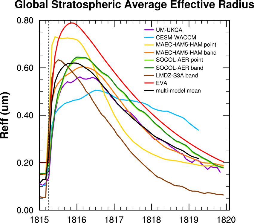
M. Clyne et al.: Model physics and chemistry causing intermodel disagreement 3319
tion. We end by providing possible ways to move forward to
address these uncertainties in future intercomparison studies.
2 Methods
The protocol for the VolMIP-Tambora ISA ensemble (Ta-
ble 5 of Zanchettin et al., 2016) called for an equato-
rial injection of 60 Tg of SO2 (equivalent to ∼ 30 TgS) on
1 April 1815 for a 24 h eruption with 100 % of the mass in-
jected between 22 and 26 km, increasing linearly with height
from zero at 22 km to max at 24 km, and then decreas-
ing linearly to zero at 26 km. Modeling groups injected at
the nearest corresponding vertical levels available on their
model vertical grid. This SO2 emission estimate is roughly
in agreement with prior petrological and ice core estimates
(e.g., Self et al., 2004; Gao et al., 2008). The 60 Tg injec-
tion also agrees with the subsequent estimate of Toohey and
Sigl (2017), who provide an uncertainty estimate of ±9 Tg
SO2 (4.5 TgS). Further explanation about the decision of the
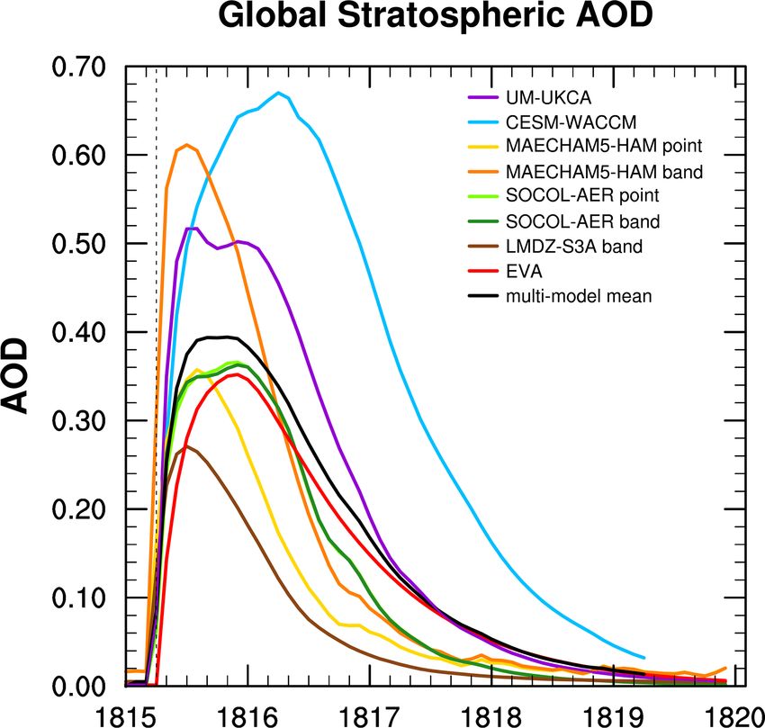
Figure 1. Ensemble mean global mean stratospheric AOD in injection parameter values used for the experimental pro-
the visible spectrum of participating models. The black line (the
tocol can be found in Marshall et al. (2018). Ensembles
VolMIP-Tambora ISA ensemble mean) is the mean of CESM-
with five members were run for 5 years producing monthly
WACCM (blue), UM-UKCA (purple), SOCOL-AER point (green),
MAECHAM5-HAM point (gold), LMDZ-S3A band (dark brown), average outputs and were started at the easterly phase of
and EVA (red) models. SOCOL-AER and MAECHAM5-HAM the quasi-biennial oscillation (QBO). Radiative forcings for
band injection experiments are in green and orange respectively. CO2 , other greenhouse gases, and tropospheric aerosols (and
Vertical dotted line marks date of injection of SO2 , which is slightly O3 if specified in the model) were set to the values each
offset from the zero AOD in the models due to the temporal reso- model uses to define preindustrial (1850) climate conditions.
lution of the model output and curve smoothing in the plotting pro- In the Community Earth System Model Whole Atmosphere
gram. Community Climate Model (CESM-WACCM), the simu-
lations were run with a preindustrial coupled atmosphere
and ocean. In the Laboratoire de Météorologie Dynamique-
Zoom Sectional Stratospheric Sulfate Aerosol (LMDZ-
suggested general reasons for the intermodel disagreement S3A) model, ECHAM-HAM in the middle-atmosphere ver-
in sulfate deposition to be MAECHAM5-HAM’s use of sion (MAECHAM5-HAM), the modeling tool for studies of
prescribed OH, intermodel differences in simulated strato- SOlar Climate Ozone Links Atmospheric and Environmen-
spheric aerosol transport that are in part due to simulated tal Research (SOCOL-AER), and the Unified Model United
stratospheric winds and horizontal model resolution, and dif- Kingdom Chemistry and Aerosol (UM-UKCA), simulations
ferences in stratosphere–troposphere exchange of aerosols did not include interactive coupling between atmosphere and
that are in part due to different deposition and sedimentation ocean but instead were run with prescribed sea-surface tem-
schemes and vertical model resolution. peratures from a previous coupled atmosphere–ocean prein-
The LMDZ-S3A model was not added to the VolMIP- dustrial control integration.
Tambora ISA ensemble until recently, after the Marshall et Some characteristics of the VolMIP-Tambora ISA models
al. (2018) paper was published. Now, our goal is to iden- are included in Table 1. One important difference between
tify and understand the causes of intermodel disagreement in the simulations is how some of the modeling groups included
the AOD itself. In this paper we go further than Marshall et additional runs with an artificial longitudinal spread of the
al. (2018) by pinpointing the primary sources of intermodel volcanic cloud. The cloud from an equatorial injection of this
inconsistencies in volcanic aerosol formation, evolution, and size into the stratosphere will fully encircle the globe within
duration in the stratosphere that largely contribute to the in- the tropics in a few weeks, spreading (in this case) westward
consistencies in modeled global stratospheric AOD. We ex- with the zonal winds from the easterly phase of the QBO
plain where and why these specific differences matter for (Robock and Matson, 1983; Baldwin et al., 2001). To investi-
AOD. We illustrate how the sources of disagreement in AOD gate the potential impact of beginning with a 2-D zonal injec-
that we identify in this paper, most crucially those relating to tion of SO2 instead of a 3-D injection that incorporates longi-
aerosol particle size whose importance was not analyzed in tude as a dimension, the MAECHAM5-HAM and SOCOL-
Marshall et al. (2018), also apply to volcanic sulfate deposi- AER modeling groups performed both “point” and “band”
https://doi.org/10.5194/acp-21-3317-2021 Atmos. Chem. Phys., 21, 3317–3343, 2021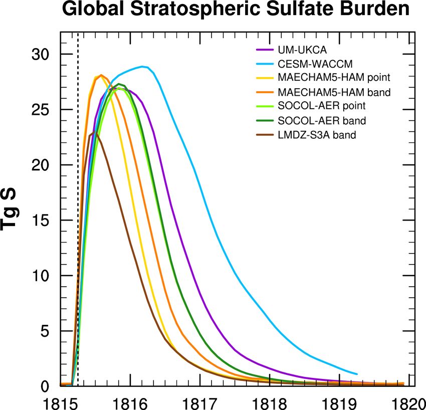
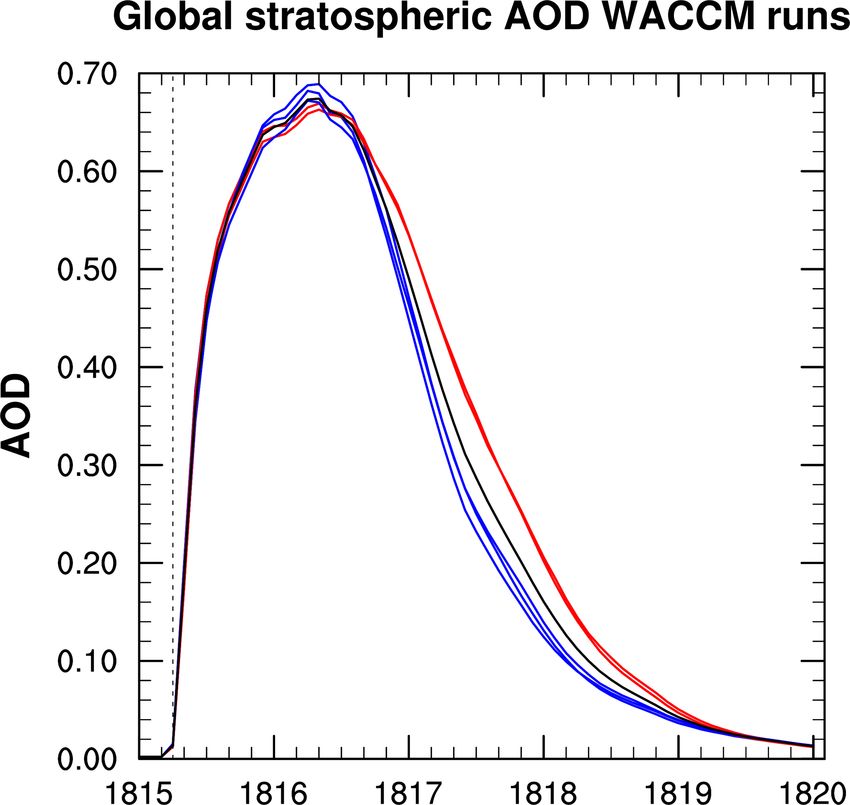
3320                                        M. Clyne et al.: Model physics and chemistry causing intermodel disagreement

experiments. We refer to a “point” injection as a grid cell at     QBO strength observed after El Chichón starting in 1982.
the Equator at the longitude of Tambora, which is located          MAECHAM5-HAM does not generate a QBO at the reso-
at 8◦ S, 118◦ E, and a “band” injection as a zonal injection       lution used here: equatorial winds are persistently easterly.
of the 60 Tg of SO2 spread evenly across all longitudes at         EVA does not account for the QBO in its transport scheme.
the grid latitude nearest to the Equator. CESM-WACCM and              After SO2 is injected in the manner described by the ex-
UM-UKCA injected the 60 Tg of SO2 as point injections.             perimental protocol, it is converted to H2 SO4 gas (sulfu-
LMDZ-S3A performed a band injection. As a 2-D scaling-             ric acid vapor) with the rate-limiting step being the reac-
based forcing generator, EVA does not follow the injection         tion with photochemically produced OH (Bekki, 1995). The
from its origins for stratospheric transport and instead uses a    strong volcanic source of H2 SO4 gas nucleates to produce an
three-box model to produce the zonally averaged spatiotem-         aerosol cloud that initially comprises very small particles (a
poral structure of the cloud. In EVA, SO2 is converted to sul-     few tens of nanometers). These then rapidly coagulate with
fate based on a fixed timescale, and effective radius is taken     each other and grow also from acid vapor condensation, to
to be proportional to aerosol mass following the observed ef-      submicrometer-sized particles (English et al., 2011; Seinfeld
fective radius evolution after Pinatubo. EVA does not take         and Pandis, 2016). In this paper we write the particle form
into account the stratospheric sulfur injection height, nor        of H2 SO4 as “SO4 ” to distinguish between the vapor phase
does it account for vertical variations in stratospheric dynam-    and the particle phase. Sulfate aerosol (SO4 ) is the species of
ics (Toohey et al., 2016). The term “VolMIP-Tambora ISA            sulfur directly relevant to AOD. More detailed descriptions
ensemble mean” refers to the average of all models except          of the sulfur chemistry can be found in the model overview
for the MAECHAM5-HAM band and SOCOL-AER band                       references cited in Table 1. The stratospheric residence time
injection experiments to avoid double counting of the same         of the sulfate is controlled by advective transport, which is
model with its point injection experiment. The postprocess-        independent of particle size, and by vertical fall velocity,
ing methods to obtain the monthly stratospheric global mean        which depends on particle size. In Sect. 3.1–3.3, we provide
values of AOD, sulfur species burdens, and effective radius        an overview of the results from the different models, focus-
are detailed in Appendix A. e-Folding lifetimes are calcu-         ing on the global mean values of stratospheric AOD, sulfate
lated as the time elapsed after reaching the maximum value         burden, and effective radius.
when the quantity crosses 1/e of its maximum. The preci-              MAECHAM5-HAM and LMDZ-S3A do not interactively
sion of these e-folding rates is limited by the time resolution    calculate OH and instead prescribe OH concentrations (Ta-
of the results, which are output every month.                      ble 2). In LMDZ-S3A, the OH fields give a stratospheric
   The models provided AOD in the visible spectrum at the          mean lifetime of about 36 d for SO2 . Because it was not in-
wavelength λ = 550 nm. The exception was SOCOL-AER,                cluded in the injection experimental protocol, none of the
which calculated the AOD output over a wider band (λ = 440         models considered an injection of water, which could im-
to 690 nm) but is still in the visible spectrum (Table 1). While   pact the OH mixing ratios, or ash which could be important
different wavelengths were used, they still fall within the Mie    for photolysis (Sect. 4.4). The impact of band injections and
scattering regime for volcanic sulfate aerosols, because the       OH chemistry on AOD, sulfate burden, and effective radius
optical size parameter of α = 2πr   λ remains within the order     are discussed in Sect. 4.2.
of 1–10 for particles of radius 0.1–1 µm. SOCOL-AER and
LMDZ-S3A use sectional size distribution schemes. The rest
of the models use modal size distribution schemes. Further         3     Results
details about the size distribution schemes used by the mod-
els can be found in Table 2 and Appendix B.                        3.1    Global-mean stratospheric AOD
   UM-UKCA produces an internally generated QBO (Ta-
ble 2) so each of its five runs has a slightly different QBO       Ensemble means of global mean stratospheric AOD outputs
strength even though they all inject the volcanic SO2 with         from participating models are plotted in Fig. 1. They are
an easterly phase in the 6 months after the injection. In          wide-ranging both in magnitude and time. For global mean
LMDZ-S3A, winds and temperatures are nudged towards                stratospheric AOD, the peak values of the models vary by
ERA-Interim reanalyses, treating the Tambora period as the         65 % above to 19 % below the multi-model mean maximum
Mt. Pinatubo period, which begins during the easterly phase        value for the original VolMIP-Tambora ISA ensemble mod-
of the QBO (i.e., starting with 1991 being 1815 and so on).        els that were included in Marshall et al. (2018), and the
SOCOL-AER and CESM-WACCM nudge the QBO to be                       peak values vary by 63 % above and 34 % below the multi-
in the easterly phase at the time of injection by nudging          model mean maximum when LMDZ-S3A is included. The
the winds in the tropics to historical observations. SOCOL-        model outputs with higher-than-average AOD are CESM-
AER uses the QBO strength observed during and after                WACCM, MAECHAM5-HAM band, and UM-UKCA. We
1991 Mt. Pinatubo. Three of the ensemble runs in CESM-             will refer to this group as “Group AODHigh”. The model
WACCM use the QBO observed after Mt. Pinatubo starting             outputs with lower than average AOD (“Group AODLow”)
in 1991, and two CESM-WACCM ensemble runs use the                  are MAECHAM5-HAM point, EVA, SOCOL-AER point,

Atmos. Chem. Phys., 21, 3317–3343, 2021                                              https://doi.org/10.5194/acp-21-3317-2021
M. Clyne et al.: Model physics and chemistry causing intermodel disagreement                                                                                                 3321

Table 1. Model overview.

     Model                          Type                Horizontal        Model top                     Injection           Optical       Reference
                                                        resolution:       (no. of levels)               region              depth λ
                                                         lat × long                                                           (nm)
     CESM-WACCM                     CCM       0.95◦ × 1.25◦ 4.5 × 10⁻⁶ hPa (70) point                                          550        Mills et al. (2016)
     UM-UKCA                        CCM      1.25◦ × 1.875◦ 0.004 hPaa (85)           point                                    550        Dhomse et al. (2014)
     SOCOL-AER                      CCM          2.8◦ × 2.8◦ 0.01 hPa (39)            point, band                          440–690        Sheng et al. (2015)
     MAECHAM5-HAM                   AGCM         2.8◦ × 2.8◦ 0.01 hPa (39)            point, band                              550        Niemeier et al. (2009)
     LMDZ-S3A                       CTM       1.89◦ × 3.75◦ 0.0148 hPa (79)           band                                     550        Kleinschmitt et al. (2017)
     EVA                                2-D scaling-based idealized volcanic forcing modelb                                    550        Toohey et al. (2016)
   a 85 km. Converted in this table to pressure using 1976 US Standard Atmosphere. b EVA output used here is at 1.8◦ latitude resolution with 31 altitude-defined vertical
   levels.

Table 2. Physics and chemistry differences of the interactive aerosol models.

                        Model                          Interactive       Aerosol size dist.                  Photorates       QBO
                                                       OH                                                    include
                                                                                                             aerosols
                        CESM-WACCM                     Yes               modal, 3 modesc                     Noi              Nudged
                        UM-UKCA                        Yes               modal, 4 modesd                     Noj              Internally generated
                        SOCOL-AER                      Yes               sectional, 40 size binse,f          Nok              Nudged
                        MAECHAM5-HAM                   Noa               modal, 3 modesg                     Nol              None
                        LMDZ-S3A                       Nob               sectional, 36 size binsh,f          Nom              Nudged
                     a Climatological concentrations of background OH values have been taken from Timmreck et al. (2003). In the stratosphere, OH,
                     NO2 , and O3 concentrations are prescribed from a climatology of the chemistry climate model MESSy (Jöckel et al., 2005).
                     b OH chemistry is not included in the model. In the stratosphere, OH concentrations are prescribed from a climatology of a
                     2-D stratospheric chemistry climate model (Bekki et al., 1993), giving a stratospheric mean lifetime of about 36 d for SO2 .
                     c CESM-WACCM modes {name, radius limits (nm), standard deviation}: {Aitken, (4.35, 26), 1.6}; {accumulation, (26.75, 240), 1.6};
                     {coarse, (200, 20000), 1.2}. Modes are composed of internal mixtures of soluble and insoluble components (“mixed/soluble”).
                     d UM-UKCA modes {name, radius limits (nm), standard deviation}: {nucleation, (, 5), 1.59}; {Aitken, (5, 50), 1.59}; {Accumulation,
                     (50, 500), 1.4}; {accumulation insoluble, (–, –), 1.59}. For volcanic stratospheric aerosols, only mixed/soluble modes are used except
                     for the accumulation-insoluble mode. See Appendix B. e From 0.39 nm to 3.2 µm. f Neighboring size bins differ by volume
                     doubling, meaning that the radius of bin i is equal to 21/3 times the radius of bin i − 1. g MAECHAM5-HAM modes {name, radius
                     limits (nm), standard deviation}: {nucleation: (, 5), 1.59}; {Aitken, (5, 50), 1.59}; {accumulation, (50, 500), 1.2}. For volcanic
                     stratospheric aerosols, only mixed/soluble modes are used. h With a dry radius ranging from 1 nm to 3.3 µm (for particles at 293 K
                     consisting of 100 % H2 SO4 ). i CESM-WACCM uses a lookup table for H2 SO4 photolysis by visible light from Feierabend et
                     al. (2006), and H2 SO4 photolysis by Lyman α from Lane and Kjaergaard (2008). j UM-UKCA uses a Fast-JX photolysis scheme by
                     Wild et al. (2000), Neu et al. (2007), and Prather et al. (2012) but does not enact the effects of volcanic aerosol on the FAST-JX
                     photolysis rate calculations. k SOCOL-AER uses a lookup table for H2 SO4 photolysis by visible light from Vaida et al. (2003) with
                     corrections from Miller et al. (2007) and H2 SO4 photolysis by Lyman α from Lane and Kjaergaard (2008). l Photolysis rates of OCS,
                     SO2 , SO3 , and O3 are prescribed based on zonal and monthly mean datasets from a climatology of the chemistry climate model
                     MESSy (Jöckel et al., 2005). m LMDZ-S3A does not include photolysis in its stratospheric chemistry (Kleinschmitt et al., 2017).

SOCOL-AER band, and LMDZ-S3A band. The mean AOD                                            CESM-WACCM are the two models that reached the high-
values for Group AODHigh and Group AODLow for the first                                    est magnitudes for stratospheric global mean AOD, CESM-
year after the injection (April 1815–March 1816) are 0.49                                  WACCM remains at AOD levels above an arbitrary value
and 0.28 respectively. The ensemble mean AOD lies between                                  of 0.1 for almost a year and a half longer than MAECHAM5-
these two subsets and is 0.36 for the first year.                                          HAM band (38 vs. 21 months). Once AOD begins to de-
   The injection of SO2 occurred on 1 April 1815. The                                      cline, CESM-WACCM and UM-UKCA have AOD e-folding
LMDZ-S3A band and MAECHAM5-HAM band injections                                             times of 17 months; EVA has 15 months; SOCOL-AER
reach their peak AOD in July 1815, with values of 0.27                                     point, SOCOL-AER band, and MAECHAM5-HAM band
and 0.61 respectively. MAECHAM5-HAM point and UM-                                          have 11 months; and MAECHAM5-point and LMDZ-S3A
UKCA peak a month later with AOD values of 0.36 and 0.53                                   band have 10 months (Table 3). Interestingly, the band injec-
respectively. SOCOL-AER point, SOCOL-AER band, and                                         tion for MAECHAM5-HAM produces twice the peak AOD
EVA peak at 0.37, 0.36, and 0.35 in December 1815, and                                     of its point injection. However, within the SOCOL-AER runs
CESM-WACCM finally peaks at 0.67 in April 1816, a full                                     there is little difference in AOD between the band and point
year after the injection. While MAECHAM5-HAM band and

https://doi.org/10.5194/acp-21-3317-2021                                                                           Atmos. Chem. Phys., 21, 3317–3343, 2021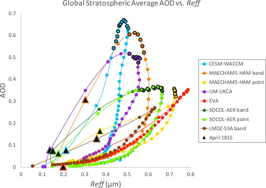
3322                                         M. Clyne et al.: Model physics and chemistry causing intermodel disagreement

                                                                    verted by the time of the first month’s output. MAECHAM5-
                                                                    HAM gives the quickest conversion time from SO2 to sulfate,
                                                                    as indicated by the short (< 1-month) e-folding stratospheric
                                                                    lifetime of SO2 and by the earliest peak in sulfate, which oc-
                                                                    curs in August 1815.
                                                                        In Table 3 we see that MAECHAM5-HAM produces
                                                                    the shortest perturbation of sulfate in the stratosphere, with
                                                                    an e-folding time of 8 months for the point injection and
                                                                    10 months for the band injection after peaking early (in
                                                                    August 1815). Sulfate burdens of the other models con-
                                                                    tinue to rise after the MAECHAM5-HAM burden has al-
                                                                    ready begun to decrease. With a longer SO2 e-folding time
                                                                    of 2 months, SOCOL-AER reaches its peak sulfate burden
                                                                    in November 1815, after which sulfate is removed at the
                                                                    same rate as in MAECHAM5-HAM’s band injection. Fig-
                                                                    ure 2 indicates that large global stratospheric burden val-
                                                                    ues of the perturbed volcanic sulfate are more stable within
                                                                    UM-UKCA and CESM-WACCM than in the other models.
                                                                    Both models give 2-month e-folding times for SO2 . Unlike
                                                                    MAECHAM5-HAM and SOCOL-AER, whose sulfate bur-
Figure 2. Global stratospheric burden of SO4 in TgS vs. time. The   dens rapidly increase until reaching a peak value, the sul-
vertical dashed black line indicates month of injection.            fate burdens of UM-UKCA and CESM-WACCM begin to
                                                                    plateau roughly 4–5 months after the injection and then in-
                                                                    crease more gradually before finally reaching their peak val-
experiments. We have detailed discussions on band and point         ues in October 1815 for UM-UKCA and March 1816 for
injections in Sect. 4.2.2.                                          CESM-WACCM (Fig. 2). The decay rate of the sulfate bur-
                                                                    den that follows is 4 months longer in UM-UKCA than
3.2     Stratospheric sulfate burden
                                                                    in MAECHAM5-HAM band and SOCOL-AER. In addi-
We split the following description of the results on strato-        tion to taking the longest time to reach its peak sulfate bur-
spheric sulfate burden into two parts. In Sect. 3.2.1 we            den value, CESM-WACCM has the longest duration of in-
present the results without including LMDZ-S3A, and then            creased sulfate burden, with an e-folding time twice that of
we separately explain the LMDZ-S3A results in Sect. 3.2.2.          MAECHAM5-HAM point. Marshall et al. (2018) find that
This is because the LMDZ-S3A sulfate burden results are             35 % of the global sulfate deposition in MAECHAM5-HAM
very different from the other models, and we do not want an         point occurs in 1815, and 60 % occurs in 1816. In SOCOL-
analysis of the variation between the remaining models to be        AER deposition starts after MAECHAM5-HAM and 75 %
overwhelmed by discussion about the differences of a single         of global sulfate deposition occurs in 1816. Only 9 % occurs
model.                                                              in UM-UKCA during 1815, and then 55 % in 1816 and 29 %
                                                                    in 1817. No sulfate deposition occurs in CESM-WACCM un-
3.2.1    Stratospheric sulfate burden without LMDZ-S3A              til 1816, when 35 % of global sulfate deposition occurs fol-
                                                                    lowed by 46 % in 1817 and 17 % in 1818, with deposition
Mass of global stratospheric sulfur is conserved in the mod-        still occurring above background levels at the end of the sim-
els with sulfur aerosol chemistry within the first several          ulation (Marshall et al., 2018).
months following the injection of SO2 , as the sums of their
volcanic sulfur species burdens (SO2 + H2 SO4 + SO4 ) sta-          3.2.2   Stratospheric sulfate burden of LMDZ-S3A
bilize at ∼ 30 TgS but then decay at different rates (Fig. S1
in the Supplement). The relevant form of volcanic sulfur for        The global stratospheric sulfate burden is noticeably lower
AOD is sulfate aerosol (SO4 ), whose global stratospheric           in LMDZ-S3A than in all of the other models (Fig. 2) and
burden time series (in TgS) is shown in Fig. 2. All of the          reaches a maximum of only 23 TgS in the band injection.
models produce peak sulfate global burdens of 27–29 TgS,            Unlike the other models, the mass of global stratospheric
but these peak values are reached at different times, and sul-      sulfur in LMDZ-S3A is not stable within the first several
fate is removed from the stratosphere at different rates.           months following the injection of SO2 ; sulfate is crossing
   Table 3 provides more insight on the sulfate burden. All         from the stratosphere into the troposphere, where it is quickly
models peak in SO2 burden at the first month of the exper-          removed. The sum of the volcanic sulfur species strato-
iment, which is in April 1815. Model outputs are provided           spheric burden (SO2 +H2 SO4 +SO4 ) exceeds 29 TgS for the
monthly, so some SO2 has already been removed or con-               first 2 months in the LMDZ-S3A band injection experiment

Atmos. Chem. Phys., 21, 3317–3343, 2021                                              https://doi.org/10.5194/acp-21-3317-2021
M. Clyne et al.: Model physics and chemistry causing intermodel disagreement                                                                                     3323

Table 3. Maximum values of global stratospheric burdens of sulfur species (TgS) and AOD: max value, month of injection experiment at
which it peaked, e-folding time in months from peak value. n/a stands for not applicable.

                                                            SO2                                     SO4                                   AOD
                                              Maxa       Monthb        e-foldc           Max       Month       e-fold         Max       Month       e-fold
          CESM-WACCM                          25.74          1              2           28.87           12         16          0.67          13       17
          UM-UKCA                             26.99          1              2           26.90            7         14          0.53           5       17
          SOCOL-AER band                      25.24          1              2           27.30            8         10          0.36           9       11
          SOCOL-AER point                     25.27          1              2           26.94            8         10          0.37           9       11
          MAECHAM5-HAM band                   19.55          1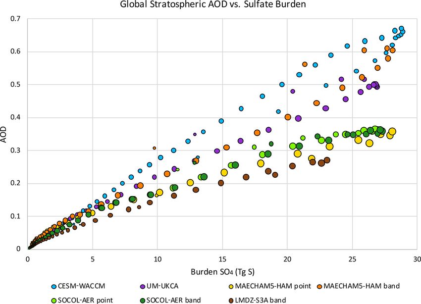
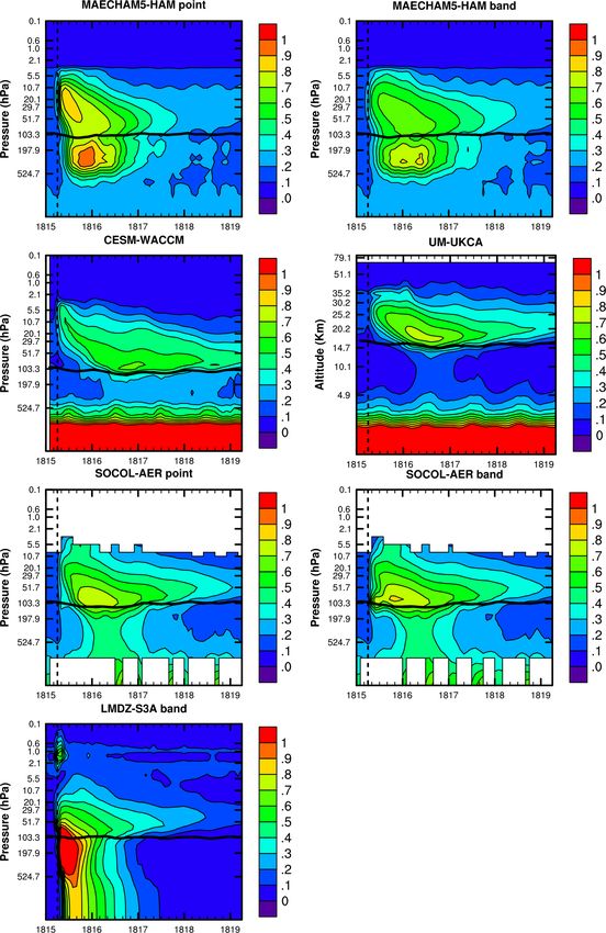
3324                                          M. Clyne et al.: Model physics and chemistry causing intermodel disagreement

Figure 4. Vertical profile of tropical mean [23◦ S, 23◦ N] effective radius contours in units of micrometers (µm) marked by the color bar. A
vertical dashed line marks the April 1815 injection. A horizontal solid black line marks tropopause height. The large particles in the lower
troposphere in this figure (CESM-WACCM and UM-UKCA) are due to background particles such as sea spray and dust.

Atmos. Chem. Phys., 21, 3317–3343, 2021                                                    https://doi.org/10.5194/acp-21-3317-2021
M. Clyne et al.: Model physics and chemistry causing intermodel disagreement                                                  3325

4     Discussion                                                  the H2 O−H2 SO4 aerosol droplet; and q is the extinction ef-
                                                                  ficiency, which is a unitless function of the ratio of effective
This VolMIP-Tambora ISA ensemble study of an idealized            radius to wavelength, and the optical constants of sulfuric
equatorial large stratospheric injection of SO2 based on the      acid water solutions (of which the refractive index changes
1815 eruption of Mt. Tambora provides insight into sig-           with ω). Equations (1) and (2) are basically exact for spheres
nificant gaps between models. These gaps are not random,          in the limit in which the particles are all the same size and
nor are they related to small details in differences between      uniformly distributed over the planet. The purpose of Eqs. (1)
models. Rather they are related to first-order differences in     and (2) is to develop a simple analysis method to under-
the physics and chemistry in the models (to be further de-        stand why the various models differ so much in computed
scribed in the following sections). One could argue that one      AOD, which is output either directly or as extinction values
should not derive a volcanic forcing parameter for global         at each level that are integrated to get AOD (Appendix A).
aerosol optical depth by averaging models which lack im-          The climate models are very complex, but the underlying
portant physics with those that have more complete physics,       physics relating the computed parameters of mass, optical
particularly when the impacts of those simplifications are        depth, and effective radius is relatively simple. A derivation
not understood. While the Marshall et al. (2018) study in-        of how Eqs. (1) and (2) are adapted from the expressions
cludes a comparison of the model results to observations of       in Seinfeld and Pandis (2016) is provided in the supplemen-
the 1815 Mt. Tambora ice core sulfate deposits, conclusions       tary info of this paper. Evidence that this simplified model
on model performance should not be drawn based on which           for global stratospheric AOD works is presented in the sec-
model or models within this VolMIP-Tambora ISA ensemble           tion called “Comparing model results of AOD to AOD re-
best simulate impacts from the eruption compared to obser-        constructed from Eqs. (1) and (2)”.
vations because there are large uncertainties for the actual         In Eq. (2), ω is present because we are tracking the mass
volcanic injection parameters. In addition, this experiment       of sulfate in the models, but the particles also contain water,
does not include volcanic injections of water or ash, which       which makes them larger. The density is present because the
can impact the volcanic forcing. This VolMIP-Tambora ISA          optics depend on the physical size of the particles rather than
ensemble uses a single prescribed set of injection parameters,    their mass. There is a large vertical gradient in ρ and ω in the
which prevents individual models from choosing their injec-       stratosphere due to the variation of the absolute amount of
tion parameters to make their results match a desired set of      water with altitude. As particles fall from the initial injection
observations. As an idealized experiment, this study serves       altitude near 26 km to the tropopause, they pick up water due
best to compare models with models. The goal of this paper        to the increasing amount of water vapor, making them less
is to understand the reasons for the intermodel disagreement      concentrated, but they also become less dense. Both changes
in both magnitude and timescale of stratospheric global AOD       make the particles larger as they drift downward. An exam-
shown in Fig. 1.                                                  ple showing the variation of ρ and ω with altitude is in the
                                                                  supplementary info of this paper (Fig. S2).
4.1    Key output variables defining AOD magnitude                   Global stratospheric mean AOD vs. global stratospheric
                                                                  sulfate burden (M) is shown in Fig. 5. Within each model,
The simulated values of AOD and Reff show that global             larger sulfate burden leads to higher AOD, which is as ex-
stratospheric average AOD is proportional to its aerosol mass     pected from Eq. (1). If ρ and ω were constant and Reff was
burden divided by effective radius. Equation (1), which is        fixed, AOD would be a linear function of sulfate burden.
adapted from Seinfeld and Pandis (2016), describes this re-       However, Fig. 5 shows that within the same model, AOD
lationship.                                                       values can vary by up to ∼ 0.1 for the same sulfate burden
             M                                                    before and after the month of peak AOD. This AOD variation
AOD = ψ ·         ,                                        (1)    is because Reff changes with time, and ρ and ω are varying
             Reff
                                                                  with the altitude of the cloud. As sulfate burden increases, the
where M is the global stratospheric mass burden of sulfate        intermodel spread of AOD grows. When the global strato-
in TgS, which is the quantity plotted in Fig. 2. The propor-      spheric sulfate burden is greater than 25 TgS different mod-
tionality scalar, ψ, is                                           els give corresponding AOD values ranging widely from 0.34
                                                                  to 0.63 (Table 4). LMDZ-S3A never reaches a global strato-
        3q (molec. weight H2 SO4 )                                spheric sulfate burden of 25 TgS (Table 3). The particles in
ψ=                                 .                       (2)    LMDZ-S3A grow large quickly and fall out of the strato-
       4ρA (molec. weight S) · ω
                                                                  sphere (Fig. 4) too early to reach a global sulfate burden near-
Here A is the surface area of the Earth, ρ is the vol-            ing those of the other models (Fig. 2). It is unclear at this time
ume density of a sulfate aerosol particle (H2 O−H2 SO4 ) in       why the particles in LMDZ-S3A grow so large in this exper-
units of grams of aerosol per volume; the molecular weight        iment. Our hypothesis is that the particles in LMDZ-S3A are
of H2 SO4 = 98.079 g mol−1 ; the molecular weight of S =          growing so large because of the equations for nucleation rates
32.065 g mol−1 ; ω is the mass fraction of sulfuric acid within   used in the model, which, compared to some of the equations

https://doi.org/10.5194/acp-21-3317-2021                                           Atmos. Chem. Phys., 21, 3317–3343, 2021
3326 M. Clyne et al.: Model physics and chemistry causing intermodel disagreement
Table 4. Global stratospheric mean when SO4 > 25 TgS. show that during the first year after the eruption (April 1815–
March 1816), intermodel variance of AOD is primarily due to
Effective AOD variance of Reff . When models agree on sulfate burden, they
radius disagree on Reff . After the first year after the injection (i.e.,
(µm) after roughly March 1816), intermodel disagreement in AOD
CESM-WACCM 0.47 0.63 is primarily due to differences in the simulated sulfate bur-
UM-UKCA 0.54 0.50 den. This narrative is seen more clearly via the dashed lines
MAECHAM5-HAM band 0.55 0.58 in Fig. 7, where LMDZ-S3A is excluded from the intermodel
SOCOL-AER point 0.62 0.36 variance, and the remaining models have a brief period when
SOCOL-AER band 0.63 0.36 they intersect in global stratospheric sulfate burden around
MAECHAM5-HAM point 0.73 0.34 October 1815. In LMDZ-S3A, much of the sulfur falls out
of the stratosphere early in the experiment due to the higher
falling velocity of the large particles that are produced in the
model. The sulfate burden in LMDZ-S3A that remains in the
used by the other models, leads to lower nucleation rates (Ap- stratosphere is much lower than the other models, which ad-
pendix C). ditionally contributes to the intermodel variance of the sulfate
Larger Reff corresponds to lower AOD (Eq. 1). In burden and the AOD (solid line in Fig. 7).
the applicable visible wavelength of 550 nm, the value In this experiment, Group AODHigh all yield smaller Reff ,
of q/Reff decreases as effective radius increases above so the aerosol particles which they produce are more opti-
0.3 µm (Fig. S3). Global stratospheric mean AOD vs. effec- cally efficient at scattering light. As a result, they all have
tive radius is shown in Fig. 6. Circles outlined in black in- higher AOD values when the sulfate burden is the same for
dicate the months for each model at which the global bur- all models (Figs. 5 and 6) than do Group AODLow. This
den of sulfate exceeds 25 TgS. During this period, the mean explains the spread in AOD magnitudes of Fig. 1, vs. the
effective radius of Group AODHigh (CESM-WACCM, UM- proximity of sulfate burden magnitudes along the same time-
UKCA, MAECHAM5-HAM band) is 0.52 µm, with a mean line in Fig. 2. For example, the UM-UKCA and SOCOL-
AOD of 0.57. The mean effective radius of Group AODLow AER models differ in magnitude by ∼ 1.4× for AOD and
without EVA or LMDZ-S3A (SOCOL-AER point, SOCOL- ∼ 0.1 µm for Reff , but they have similar sulfate burdens and
AER band, MAECHAM5-HAM point) is 0.66 µm with a closely matching rates of rise and decay of AOD and Reff .
mean AOD of 0.35. Although SOCOL-AER calculated AOD CESM-WACCM and UM-UKCA aerosols never grow past a
over the range λ = 440 to 690 nm, instead of at λ = 550 nm, global stratospheric mean effective radius of 0.5 and 0.56 µm,
the different wavelength is not very important for comparing which contributes to their longer e-folding times for sulfate
AOD magnitudes across models because of the Mie scatter- burden and AOD compared to the other models. The sulfate
ing properties. The value of q (and q/Reff ) for a given ef- burden e-folding time is longer because smaller particles will
fective radius at λ = 550 nm falls in the middle of the values not sediment as quickly as larger particles.
between λ = 440 and λ = 690 nm.
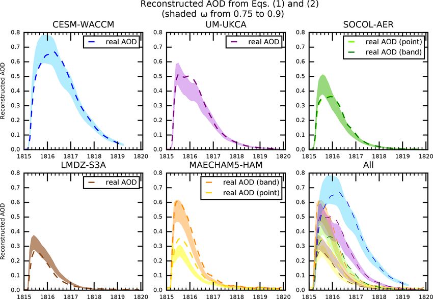
VolMIP-Tambora ISA ensemble models agree relatively Comparing model results of AOD to AOD reconstructed
well on sulfate burden during the first year after the injec- from Eqs. (1) and (2)
tion, especially toward the end of 1815, but largely disagree
on AOD. If LMDZ-S3A is excluded, the spread of the peak Operationally, ω is the only unknown value when recon-
global mean stratospheric values from individual models is structing AOD using Eqs. (1) and (2) for the VolMIP models.
only 8 % above to 1 % below the multi-model mean maxi- Values of M and Reff are known outputs from the VolMIP
mum for sulfate burden, vs. 56 % above to 19 % below the models. Values of q are calculated by Mie theory using in-
multi-model mean maximum for AOD. Figure 5 emphasizes puts of effective radius, wavelength set at 550 nm, and ω (to
the disagreement between models on global AOD values for determine the complex refractive index of the aerosol). The
a given sulfate burden. Therefore, Reff , which is the other global stratospheric average values of q are then calculated
major component of the AOD equation, Eq. (1), must be a in the same weighted average method as is done for Reff
key contributing factor to this intermodel disagreement dur- in Eq. (A3). Myhre et al. (2003) show that ρ can be cal-
ing the first year after the injection. The peak Reff values from culated using a polynomial expansion equation with inputs
the individual models vary by 25 % above to 20 % below of ω and temperature. In the applicable temperature range
the maximum value of the multi-model mean. When LMDZ- for the stratosphere and locations of the volcanic aerosol,
S3A is included these values change to 12 % above to 11 % ρ is primarily a function of ω. Plots of reconstructed global
below for sulfate burden, to 63 % above to 34 % below for stratospheric average AOD using Eqs. (1) and (2) are shown
AOD, and remain the same for Reff . The time series showing by the shaded regions in Fig. 8. The actual ω values were
how the models differ on AOD, sulfate burden, and Reff is not output by the VolMIP models at the time, so the recon-
plotted in Fig. 7. The plots of normalized intermodel variance structions in Fig. 8 were instead made using a single value
Atmos. Chem. Phys., 21, 3317–3343, 2021 https://doi.org/10.5194/acp-21-3317-2021M. Clyne et al.: Model physics and chemistry causing intermodel disagreement 3327 Figure 5. Global stratospheric AOD in the visible vs. sulfate burden from VolMIP-Tambora ISA ensemble means. Circle size is scaled by π(Reff )2 . Figure 6. Global stratospheric mean AOD in the visible vs. effective radius (µm). Points are connected in order (clockwise) of monthly values from January 1815–April 1819. Circles with black outlines are for months when global stratospheric sulfate burden > 25 TgS. The injection date of April 1815 is indicated by triangles. for ω prescribed throughout the stratosphere. The shading Fig. 8. CESM-WACCM and SOCOL-AER follow the lower in Fig. 8 for each VolMIP model encompasses the recon- part of the shaded region in the first few months, and then structed AOD calculated using ω ranging from 0.9 (lower the upper part later. This behavior is consistent with the bulk edge of the shading) to ω = 0.75 (upper edge of the shad- of the aerosols having a high weight of sulfuric acid per- ing). For comparison, the actual AOD from the VolMIP mod- cent initially, and then a lower weight percent as they fall els (i.e., the AOD in Fig. 1) is plotted as the dashed lines in downward into air with higher water concentration. Even https://doi.org/10.5194/acp-21-3317-2021 Atmos. Chem. Phys., 21, 3317–3343, 2021
3328                                             M. Clyne et al.: Model physics and chemistry causing intermodel disagreement

                                                                          aerosol (ω), the number of optically active particles should
                                                                          vary by a factor of 13 . For the Reff difference between
                                                                                                 Reff
                                                                          Groups AODHigh and AODLow, this translates to about a
                                                                          factor of 2. The global aerosol mass is almost the same for
                                                                          the various models 6 months after the eruption except for
                                                                          LMDZ-S3A (Figs. 2 and 7b), but the effective radius varies
                                                                          from about 0.7 µm for MAECHAM5-HAM point to about
                                                                          0.45 µm for CESM-WACCM (Fig. 3). It thus follows that
                                                                          either the width of the size distributions is highly variable
                                                                          between models (Sect. 4.3.1), or the number of particles is
                                                                          highly variable. More, smaller particles could be generated
                                                                          by a faster nucleation rate, a more prolonged period of new
                                                                          particle formation (Sect. 4.2.1), or a slower coagulation rate
                                                                          perhaps due to more rapid dispersion of the cloud over the
                                                                          planet (Sect. 4.2.2). Unfortunately, it is difficult to use parti-
                                                                          cle number, which was not a variable output by the models in
                                                                          this experiment, as a parameter to understand optical proper-
                                                                          ties because there can be large numbers of particles in freshly
                                                                          nucleating clouds that are optically ineffective. A third op-
                                                                          tion is that the models differ in their handling of ω, which is
                                                                          discussed in Sect 4.3.3.

                                                                          4.2.1   Interactive OH

                                                                          The rate at which SO2 is converted to sulfate, which is con-
                                                                          trolled by the OH abundance, impacts the particle effective
                                                                          radius in a number of ways. Rapid production of sulfuric acid
                                                                          leads to high nucleation rates and high growth rates, which
                                                                          ultimately lead to larger particles. Slow production of sulfu-
Figure 7. Variance between VolMIP-Tambora ISA ensemble mod-               ric acid reduces the nucleation and growth rates, generally
els for global mean stratospheric (a) AOD, (b) sulfate burden, and        leading to smaller particles. Table 2 shows which models in-
(c) effective radius. All models are included in the solid line. All
                                                                          clude interactive OH chemistry. After a large volcanic erup-
models except for LMDZ-S3A are included in the dashed line. In
                                                                          tion, the reaction of SO2 with OH locally depletes the con-
both cases (solid and dashed lines), the plots have been normal-
ized to the maximum value of the intermodel variance of all models        centration of OH, which is a limiting reactant in the conver-
(including LMDZ-S3A) at each corresponding variable. The peak             sion from SO2 to H2 SO4 . These reductions are not small.
values for the dashed line which are therefore slightly cut off from      Zhu et al.’s (2020) WACCM simulations have a reduction
view by the y axis of the subplots for the sulfate burden and effective   of a factor of 2 in OH in the volcanic plume one day after
radius are (b) 1.03 and (c) 1.16. Sulfate burden and effective radius     the small 2014 Mt. Kelut eruption (VEI of 4, stratospheric
are two of the key output variables dominating the AOD equation,          injection of ∼ 0.2–0.3 Tg SO2 ), while Mills et al. (2017;
Eq. (1), which generate intermodel variance of AOD.                       Michael Mills, personal communication, 2020) find a > 95 %
                                                                          reduction in OH in the first weeks of the evolving Pinatubo
                                                                          plume. However, although the chemistry is simple, there are
with using global stratospheric average values for M, Reff ,              no measurements of the OH depletion in volcanic clouds,
q, and (prescribed) ω, Eqs. (1) and (2) do surprisingly well              and for that matter OH is not directly measured in the lower
to match the AOD that was derived by the VolMIP models.                   stratosphere. LeGrande et al. (2016) suggested that volcanic
This gives credibility to the discussions comparing and con-              water injections could be important for OH. The reaction of
trasting global stratospheric average values of sulfate burden            O1 (D) with water frees OH and counteracts the OH depletion
and effective radius across models in the results (Sect. 3).              by SO2 . By supplementing OH mixing ratios, an injection of
                                                                          water into the stratosphere from an eruption could reduce the
4.2    Major simplifying assumptions made in models                       impact of limited OH on stratospheric chemistry. However,
       which caused these differences                                     in modeling studies of the Toba supervolcano eruption for
                                                                          a SO2 injection roughly 10 times that of Tambora, Bekki et
Next, we look at why the models disagree on sulfate bur-                  al. (1996) show that an injection of water does not completely
den and effective radius. For a fixed size distribution, mass             counteract the OH depletion by SO2 . Zhu et al. (2020) find
burden, and mass fraction of sulfuric acid within the sulfate             that a water injection orders of magnitude greater than ob-

Atmos. Chem. Phys., 21, 3317–3343, 2021                                                     https://doi.org/10.5194/acp-21-3317-2021
M. Clyne et al.: Model physics and chemistry causing intermodel disagreement 3329
Figure 8. Reconstructed global stratospheric AOD time series using Eqs. (1) and (2). Shaded regions for each model are from ω = 0.9 (lower
edge of shaded region) to 0.75 (upper edge of shaded region). The real AOD from each model is also shown (dashed lines). The dashed
lines in this plot are equivalent to the lines in Fig. 1. For this plot, the corresponding values of ρ from ω used for Eq. (2) are calculated
using the relationship described by Myhre et al. (2003). The light and dark green dashed lines (and shading) for the SOCOL-AER real (and
reconstructed) AOD plot are indistinguishable from each other because the values from the point and band injections are overlapping.
served from Kelut is needed to provide enough OH to coun- for SO2 oxidation was significantly prolonged. We infer
teract the loss from SO2 chemistry. Interactive OH is still that the lack of interactive OH in MAECHAM5-HAM and
needed in models regardless of whether or not an injection LMDZ-S3A is a significant cause of why the global sulfate
of water also occurs. In the VolMIP-Tambora ISA ensemble peaks at least 3 months earlier in them than in any of the
experiment there is no injection of water to limit the impact other models. In Sect. 4.2.2 we discuss the impacts that an
of SO2 depleting OH. Instead of comparing models to ob- earlier production of sulfate has on Reff in a band vs. point
servations, we compare model outputs with each other. In injection.
the VolMIP-Tambora ISA ensemble experiment, local de-
pletion of OH occurs in all of the models that have inter- 4.2.2 Grid cell (“point”) vs. zonal (“band”) injections
active OH chemistry: CESM-WACCM, SOCOL-AER, and
UM-UKCA (Marshall et al., 2018). EVA is not an interactive
The inclusion of band injections was performed to determine
aerosol model and thus does not include full sulfur chem-
if the initial spatial distribution of the volcanic injection mat-
istry, and OH chemistry is not applicable. In MAECHAM5-
ters. The degree to which spatial distribution matters depends
HAM and LMDZ-S3A, the OH is prescribed in background
on whether the oxidation rate for SO2 is longer or shorter
climatological concentrations and is thus not depleted from
than the several weeks needed for the SO2 to be transported
the eruption. In studies of the Toba eruption, when interactive
around the Earth and become partially homogenized. If the
stratospheric OH chemistry was included, the transition from
SO2 oxidation time is short, then the nucleation rate, coag-
SO2 to H2 SO4 was delayed, yielding a longer-lasting peak
ulation rate, and growth rate would also need to be fast for
concentration of sulfate. The limited OH resulted in a longer
there to be a difference between the results of point and band
lifetime of the volcanic cloud (Robock et al., 2009; Bekki et
injections. Since we see the sulfate forming soon after the
al., 1996; Bekki 1995; Pinto et al., 1989). A study based on
SO2 is lost in the VolMIP models, the nucleation rate, coagu-
Mt. Pinatubo by Mills et al. (2017) using CESM/WACCM
lation rate, and growth rate are rapid because the bulk of the
supported the idea that if local depletion of OH occurred
sulfur is not sitting in the H2 SO4 vapor phase. The difference
within the volcanic cloud of SO2 , the e-folding decay time
between point and band injections in SOCOL-AER is in-
https://doi.org/10.5194/acp-21-3317-2021 Atmos. Chem. Phys., 21, 3317–3343, 20213330 M. Clyne et al.: Model physics and chemistry causing intermodel disagreement
significant, probably because the SO2 stratospheric lifetime 4.3 Other model uncertainties
in the experiment in this model is longer (2-month e-folding
decay time) than the time needed to transport the SO2 . As a The CESM-WACCM, SOCOL-AER point, and UM-UKCA
result, the gas from a point injection can form a band before models do have interactive OH chemistry and do not use
much sulfate is produced from the oxidation of SO2 . How- band injections. Yet, their results still vary in AOD, sulfate
ever, in MAECHAM5-HAM the band injection experiment mass, and effective radius. Further explanations are there-
has an AOD twice as high as its point injection, which is ul- fore needed to understand these disparities. Table 2 shows a
timately due to the short stratospheric lifetime of the SO2 in number of additional differences between the models, which
this model (< 1-month e-folding time), which is on the same relate to the setup of the model’s size distribution, to photol-
timescale as the transport time. For the band injection, the ysis, and to stratospheric meridional transport and may con-
lower concentration of sulfuric acid and water vapor presum- tribute to remaining inconsistencies.
ably causes less nucleation and condensational growth than
for the point injection, and the corresponding lower concen- 4.3.1 Size distribution scheme
tration of the sulfate aerosols leads to less coagulation. As a
First, there are differences in the ways in which the mod-
result, the band injection experiment in MAECHAM5-HAM
els treat the aerosol size distribution (Table 2, Appendix B).
produces aerosol particles with smaller effective radii, which
Modal models assume a lognormal size distribution, whose
are more efficient optically and have lower falling velocity,
mean size is allowed to vary, but whose width is fixed. Sec-
thus resulting in higher AOD with a longer e-folding time.
tional models define the size distribution using a fixed set of
The geoengineering studies by Niemeier et al. (2011)
size bins, usually resolved over a logarithmic grid, and allow
and Niemeier and Timmreck (2015) using ECHAM5-HAM
the number concentration within each size bin to vary. Modal
reached the opposite conclusion; they found that increas-
models suffer from sensitivity to choice in mode width, and
ing the injection area by using a band injection instead of a
sectional models may not resolve the distributions well by
point injection resulted in larger Reff and lower AOD. These
having too few bins. Kokkola et al. (2009) found the differ-
geoengineering studies noted that the lower concentration
ences in results arising from these limitations to be enhanced
of SO2 and more equally distributed H2 SO4 in their band
with larger volcanic injections of SO2 . In a separate study,
injection (interactive OH was not included in their simula-
Weisenstein et al. (2007) performed a global 2-D intercom-
tions) led to condensation occurring on pre-existing parti-
parison of sectional and modal aerosol models by contrast-
cles rather than to nucleation, causing lower particle num-
ing 20-, 40-, and 150-bin sectional models with 3- and 4-
bers with larger Reff . However, the geoengineering studies
mode modal models in simulations for ambient stratospheric
were for continuously emitted SO2 at rates of 4 and 10 TgS
sulfate, and for the Pinatubo volcanic cloud. They found sig-
of SO2 per year, which is much lower in concentration than
nificant errors in using modal models unless care was taken
the 60 TgS of SO2 injected over 24 h in this VolMIP-Tambora
in the width of the modes, and that none of the modal mod-
ISA study, and still lower in concentration than more com-
els considered compared well with the sectional model for
mon Pinatubo-sized volcanic events due to the temporal
effective radius. English et al. (2013) explored the variation
emission scale. Continuously emitting SO2 instead of inject-
of lognormal fits to simulated size distribution and found that
ing SO2 in pulses can significantly affect the size of the sul-
the widths change with size of eruption, time, and location. A
fate particles (Heckendorn et al., 2009) because they add to
new aerosol microphysics model, SALSA2.0 (Kokkola et al.,
the particles already present rather than making many more.
2008, 2018), was implemented in another study (Kokkola et
Similarly, a volcanic injection into high sulfate background
al., 2018) as an alternative microphysics model to the default
levels would result in larger particles (Laakso et al., 2016).
modal scheme in ECHAM-HAMMOZ. They found that the
Volcanic eruption studies such as this VolMIP-Tambora ex-
sectional model was able to reproduce the observed time evo-
periment inject SO2 into low sulfate background concentra-
lution of the global sulfate burden and stratospheric aerosol
tions. Thus, the use of geoengineering studies as an analog
effective radius slightly better compared to the modal aerosol
for volcanic eruptions should be taken with care. Generaliza-
scheme in their simulations of the 1991 Pinatubo eruption.
tions from geoengineering studies in terms of the results of
We suggest, for each model in this VolMIP-Tamborra ISA
horizontal injection area should not be applied to modeling
ensemble that has the option to use a sectional or modal
volcanic events, as we find that volcanic injections of SO2
model in its aerosol size distribution scheme, running this
into low sulfate background concentrations give opposite re-
same Tambora experiment using its counterpart, so that the
sults between using band injections compared to point injec-
differences in produced Reff from the choice of aerosol size
tions than do geoengineering studies of continuously injected
distribution scheme might be further assessed. At this time,
SO2 .
we cannot make any conclusions about whether the use of
modal vs. sectional size distribution schemes plays a role in
the intermodel disagreement of the VolMIP-ISA models in
this experiment.
Atmos. Chem. Phys., 21, 3317–3343, 2021 https://doi.org/10.5194/acp-21-3317-2021You can also read