MOMSO 1.0 - an eddying Southern Ocean model configuration with fairly equilibrated natural carbon - Geosci. Model Dev.
←
→
Page content transcription
If your browser does not render page correctly, please read the page content below
Geosci. Model Dev., 13, 71–97, 2020
https://doi.org/10.5194/gmd-13-71-2020
© Author(s) 2020. This work is distributed under
the Creative Commons Attribution 4.0 License.

MOMSO 1.0 – an eddying Southern Ocean model configuration
with fairly equilibrated natural carbon
Heiner Dietze1,2 , Ulrike Löptien1,2 , and Julia Getzlaff1
1 GEOMAR,        Helmholtz Centre for Ocean Research Kiel, Düsternbrooker Weg 20, Kiel, Germany
2 Institute   of Geosciences, University of Kiel, Kiel, Germany

Correspondence: Heiner Dietze (hdietze@geomar.de)

Received: 23 November 2018 – Discussion started: 11 January 2019
Revised: 6 November 2019 – Accepted: 28 November 2019 – Published: 9 January 2020

Abstract. We present a new near-global coupled biogeo-            Subantarctic waters. This definition is straightforward be-
chemical ocean-circulation model configuration. The config-       cause it characterizes the transition from one oceanographic
uration features a horizontal discretization with a grid spac-    regime to another distinctly different one. However, because
ing of less than 11 km in the Southern Ocean and gradu-           the position of the front varies with time, the definition adds
ally coarsens in meridional direction to more than 200 km at      complexity to certain analyses such as oceanic inventories. A
64◦ N, where the model is bounded by a solid wall. The un-        pragmatic solution is to define a fixed latitude as the northern
derlying code framework is the Geophysical Fluid Dynam-           boundary. We choose 40◦ S in order to facilitate a comparison
ics Laboratory (GFDL)’s Modular Ocean Model coupled to            with, e.g., Lovenduski et al. (2013) and Dietze et al. (2017).
the Biogeochemistry with Light, Iron, Nutrients and Gases            The atmospheric conditions in the Southern Ocean are
(BLING) ecosystem model of Galbraith et al. (2010). The           characterized by frequent cyclonic storms that travel east-
configuration is unique in that it features both a relatively     ward around the Antarctic continent and high-pressure ar-
equilibrated oceanic carbon inventory and an eddying ocean        eas over the poles. This averages to a strong westerly wind
circulation based on a realistic model geometry/bathymetry        belt between 40 and 60◦ S, and rather weak and irregular
– a combination that has been precluded by prohibitive com-       polar easterlies from 60◦ S on southwards. The dominant
putational cost in the past. Results from a simulation with       low-frequency mode of atmospheric variability is summa-
climatological forcing and a sensitivity experiment with in-      rized by the Southern Annular Mode (Limpasuvan and Hart-
creasing winds suggest that the configuration is sufficiently     mann, 1999; Marshall, 2003) which essentially describes the
equilibrated to explore Southern Ocean carbon uptake dy-          strength and position of the westerly wind belt.
namics on decadal timescales. The configuration is dubbed            The strong westerly wind belt drives the Antarctic Circum-
MOMSO, a Modular Ocean Model Southern Ocean configu-              polar Current (ACC), the “mightiest current in the oceans”
ration.                                                           (Pickard and Emery, 1990), which is unobstructed by conti-
                                                                  nents. The ACC circumnavigates the globe zonally and thus
                                                                  links the Atlantic, Pacific and Indian oceans. Northward Ek-
                                                                  man transport (also driven by the westerlies) drives up- and
1   Introduction                                                  downwelling (Marshall and Speer, 2012) and is part of a
                                                                  meridional overturning circulation. Among the major pro-
The Southern Ocean, also known as the Antarctic Ocean,            cesses controlling the net overturning is the so-called “eddy
comprises the southernmost waters of the world oceans. Its        compensation” which largely cancels changes in wind-driven
southern boundary is set by the Antarctic continent. With re-     overturning (see Marshall and Radko, 2003; Viebahn and
gard to its northern boundary to the Atlantic, Pacific and In-    Eden, 2010; Abernathey et al., 2011, 2016; Hallberg and
dian oceans, there is no consensus. One common definition         Gnanadesikan, 2006; Thompson et al., 2014; Tamsitt et al.,
is the location of the Subtropical Front (STF), which sepa-       2017). Further complexity is added by sea ice which modu-
rates the relatively saline subtropical waters from the fresher

Published by Copernicus Publications on behalf of the European Geosciences Union.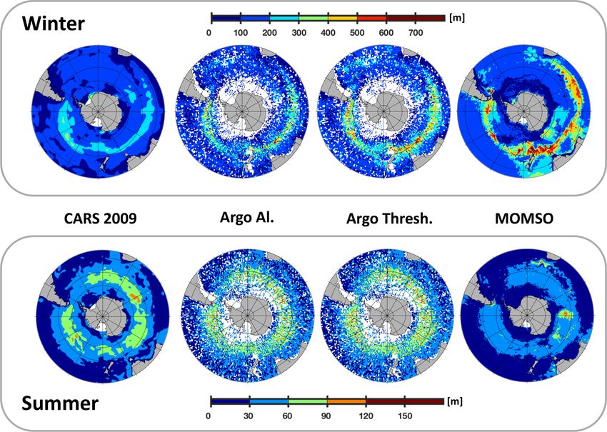
72                                                                                               H. Dietze et al.: MOMSO 1.0

lates air–sea buoyancy fluxes and thus exerts control on con-     2002) that this model behavior is a spurious consequence
vection, a prerequisite for Antarctic Bottom Water (AABW)         of the underlying eddy parameterization in coarse-resolution
formation.                                                        models which cannot afford to resolve mesoscale dynam-
   Being one of the few places worldwide where deep wa-           ics explicitly. Supporting evidence came from Munday et al.
ter (such as AABW) is formed, the Southern Ocean plays a          (2014), who showed that mesoscale eddies indeed reduce the
major role in the global carbon budget. Convection events         sensitivity of oceanic carbon sequestration towards changing
tap into the abyssal ocean and modulate the difference be-        wind stress in an idealized model.
tween atmospheric and oceanic CO2 concentrations which               To date, we know that very different state-of-the-art ap-
drive net air–sea fluxes. A comprehensive quantitative un-        proaches to parameterize eddies yield surprisingly similar
derstanding has not been reached yet, but there is consensus      sensitivities of oceanic carbon inventories to changing winds
that the variability in the extent to which deep-water masses     (Dietze et al., 2017). Further, it has been demonstrated that
in the Southern Ocean are isolated from the atmosphere is         “the conversion of dense waters back to light waters is sen-
among the major drivers regulating atmospheric CO2 vari-          sitive to the degree of parameterization of mesoscale eddies
ability (e.g., Anderson et al., 2009; van Heuven et al., 2014;    in models” (Spence et al., 2010, 2009). The question, how-
Ritter et al., 2017). Consequently, the Southern Ocean has        ever, as to how a realistic (as opposed to one featuring an
shifted into the limelight of climate research (DeVries et al.,   idealized geometry) high-resolution coupled biogeochemi-
2017; Tamsitt et al., 2017; Langlais et al., 2017, and many       cal ocean-circulation model that actually resolves eddies and
more).                                                            carbon dynamics explicitly compares to a coarse-resolution
   To date, the Southern Ocean accounts for almost half of the    model has not been answered yet. Among the reasons is the
global oceanic CO2 uptake from the atmosphere (Takahashi          prohibitive computational cost that is associated with equili-
et al., 2012). But there is concern that anticipated climate      brating simulated dissolved inorganic carbon concentrations
change (e.g., via changes of atmospheric circulation and sea      specifically in the deep ocean.
ice cover) may trigger substantial changes in the Southern           In this model description paper, we present the realis-
Ocean carbon budget (e.g., Heinze et al., 2015; Abernathey        tic high-resolution Modular Ocean Model Southern Ocean
et al., 2016) such that the current rate of uptake may well       model configuration (MOMSO 1.0). The configuration fea-
decline in decades to come. Indications for the existence of      tures a realistic topography and simulated levels of eddy ki-
such potential triggers have been revealed by observation-        netic energy which do not undercut observed values. The lat-
based atmospheric reanalysis products which show an ongo-         ter suggests that the configuration explicitly resolves a sub-
ing strengthening and a poleward shift of the southern west-      stantial part of mesoscale-related variability rather than rely-
erly winds starting from the 1970s (Thompson and Solomon,         ing on parameterizing their effect. MOMSO is designed to
2002).                                                            explore the sensitivity of the Southern Ocean carbon uptake
   This observed trend is projected by climate scenarios to       to atmospheric changes on decadal scales. The configuration
intensify (e.g., Simpkins and Karpechko, 2012), and it is         is rendered feasible by recent advances in compute hardware
straightforward to assume that the associated wind-driven         and by its similarity to a spun-up coarse-resolution model
circulation affects biogeochemical dynamics and, eventually,      which delivered the initial conditions for the biogeochemical
the oceanic carbon budget. A comprehensive understanding          module. (Note that module refers to the algorithmic entity
of the link between changing winds and oceanic upwelling of       that calculates the local biogeochemical sources and sinks
carbon-rich deep water (which, in turn, affects surface satu-     of the prognostic biogeochemical variables such as nutrients
ration and net air–sea CO2 exchange) has, however, not been       and carbon. The algorithmic entity comprises both the un-
achieved yet. To this end, the role of mesoscale ocean ed-        derlying partial differential equations and their approximated
dies is especially uncertain: the current generation of coarse-   representation within the numerical solver.) More specifi-
resolution (non-mesoscale-resolving) models suggests that a       cally, we will showcase that the “level of equilibration” of
poleward shift and an intensification of the Southern Ocean       simulated dissolved inorganic carbon allows us to test the
westerlies results in a strengthening of the subpolar merid-      sensitivity of the Southern Ocean carbon budget to antici-
ional overturning cell (e.g., Saenko et al., 2005; Hall and       pated climate change patterns.
Visbeck, 2002; Getzlaff et al., 2016) and, consequently, in          In summary, this model description paper aims to (1) de-
increased upwelling of deep water south of the circumpo-          scribe a new eddying coupled ocean-circulation biogeochem-
lar flow, which is rich in dissolved inorganic carbon (e.g.,      ical model configuration of the Southern Ocean and (2) out-
Zickfeld et al., 2007; Lenton and Matear, 2007; Lovenduski        line research questions for which MOMSO may serve as the
et al., 2008; Verdy et al., 2007). The net effect here is that    base of a tool bench.
changes of the atmospheric circulation reduce the capabil-           The project is dubbed MOMSO, a configuration of the
ity of the Southern Ocean to sequester carbon away from the       Geophysical Fluid Dynamics Laboratory (GFDL)’s Modu-
atmosphere. Early on, however, there were indications (e.g.,      lar Ocean Model version 4p1 with enhanced resolution in the
Böning et al., 2008; Hallberg and Gnanadesikan, 2006; Hogg        Southern Ocean. The naming is a homage to the underlying
et al., 2008; Screen et al., 2009; Thompson and Solomon,          framework, the MOM4p1 release of NOAA’s GFDL Mod-

Geosci. Model Dev., 13, 71–97, 2020                                                   www.geosci-model-dev.net/13/71/2020/
H. Dietze et al.: MOMSO 1.0                                                                                                         73

ular Ocean Model (Griffies, 2009). The ocean-circulation              varies with time:
model is coupled to a sea ice model and the Biogeochem-
                                                                                z−η
istry with Light, Iron, Nutrients and Gases (BLING) model             z? = H                                                       (1)
from Galbraith et al. (2010).                                                   H +η
                                                                      (Eq. 6.6 in Griffies, 2009). The approach overcomes the
                                                                      problem with vanishing surface grid boxes which appears in
                                                                      generic z-level discretization when sea surface height varia-
2     Model setup
                                                                      tions are of similar magnitude to the thickness of the upper-
                                                                      most grid box.
This model description paper describes simulations with the
Modular Ocean Model (MOM), version MOM4p1 coupled                     2.2   Ocean circulation
to the Sea Ice Simulator (SIS) (Griffies, 2009). The config-
uration is near global, bounded by Antarctica and 64◦ N. In           MOM4p1 is a z coordinate, free-surface ocean general circu-
the Southern Ocean, the horizontal resolution is higher than          lation model which discretizes the ocean’s hydrostatic primi-
11 km. From 40◦ S, the meridional grid resolution coarsens            tive equations on a fixed Eulerian grid. The vertical mixing of
towards the north (Fig. 1). There are no open boundaries and          momentum and scalars is parameterized by the k-profile pa-
there is no tidal forcing.                                            rameterization approach of Large et al. (1994) with the same
   The biogeochemical model BLING (Galbraith et al., 2010)            parameters applied in eddy-permitting global configurations
is coupled online to the ocean–sea ice model. Atmospheric             of Dietze and Kriest (2012), Dietze and Loeptien (2013), Di-
CO2 concentrations are prescribed to a pre-industrial level of        etze et al. (2014), and Liu et al. (2010). The relevant param-
278 ppmv. The respective carbon inventories and fluxes are            eters are (1) a critical bulk Richardson number of 0.3 and
referred to as “natural carbon”.                                      (2) a constant vertical background diffusivity and viscosity
                                                                      of 10−5 m2 s−1 . These background values apply also below
2.1    Grid and bathymetry                                            the surface mixed layer throughout the water column. Both
                                                                      parameterizations of the non-local and the double diffusive
The underlying bathymetry is ETOPO5 (see Data Announce-               (vertical) scalar tracer fluxes are applied.
ment 88-MGG-02, Digital relief of the Surface of the Earth.              We apply a state-dependent horizontal Smagorinsky vis-
NOAA, National Geophysical Data Center, Boulder, Col-                 cosity scheme (Griffies and Hallberg, 2000; Smagorinski,
orado, 1988). Using a bilinear scheme, the bathymetry is              1963, 1993) to keep friction at the minimal level necessitated
interpolated onto an Arakawa B grid (Arakawa and Lamp,                by numerical stability. We apply a respective coefficient that
1977) with 2400 × 482 tracer grid boxes in the horizontal.            sets the scale of the Smagorinsky isotropic viscosity to 0.01.
The ocean-circulation and sea ice models share the same hor-          Note that this value is much smaller than the range between 2
izontal grid.                                                         and 4 recommended by Griffies and Hallberg (2000) for sta-
    The vertical discretization comprises a total of 55 levels.       bility reasons. The rationale behind our choice is to minimize
Figure 1 shows the nominal depth and thickness of each                friction which has little physical justification and at the same
level. The model bathymetry is smoothed with a filter similar         time has been shown to degrade the performance of ocean-
to the Shapiro filter (Shapiro, 1970). The filter weights are         circulation models (e.g., Jochum et al., 2008).
0.25, 0.5 and 0.25. The filtering procedure can only decrease            We use the PPM (piecewise parabolic method) advection
the bottom depth; i.e., essentially, it fills rough holes. The fil-   scheme (Colella and Woodward, 1984) for active tracers be-
ter is applied three times consecutively because we found this        cause it has been shown to perform well in treating sharp
to be a good compromise between unnecessary smoothing on              gradients in small-scale circulation (e.g., Carpenter Jr. et al.,
the one hand and numerical instabilities introduced by overly         1989). For the biogeochemical tracers, we use a flux-limited
steep topography on the other hand in other high-resolution           scheme following Sweby (1984) because we experienced
model configurations (Dietze and Kriest, 2012; Dietze et al.,         problems in the past with other configurations where negative
2014). The resulting bathymetry contained lakes which we              values occurred for biogeochemical tracers when using non-
filled after visual inspection. In addition, we filled narrow in-     flux-limited schemes. The choice of two different advection
lets which had a width of less than three grid boxes. In total,       schemes may have repercussions. For example, Lévy et al.
MOMSO has 42 429 759 wet tracer grid boxes.                           (2001) have shown that the choice spuriously affects biogeo-
    We use the zstar coordinate in the vertical (Stacey et al.,       chemistry in regions of sharp vertical macronutrient gradi-
1995; Adcroft and Campin, 2004) which is essentially an               ents such as in oligotrophic regions. We expect that this is not
extension of the non-linear free-surface method of Campin             so much an issue in MOMSO because the Southern Ocean
et al. (2004) to all model levels. The algorithm is well-             vertical nutrient gradients are smoother. Further, we argue
established for its very accurate conservation of tracers. zstar      that all advection schemes introduce spurious errors (either
(z? ) is calculated as a function of nominal depth (z), respec-       of diffusive or dispersive nature). These are directly related
tive water depth (H ) and the free sea surface height (η) which       to the respective property gradient in flow direction. Since

www.geosci-model-dev.net/13/71/2020/                                                          Geosci. Model Dev., 13, 71–97, 2020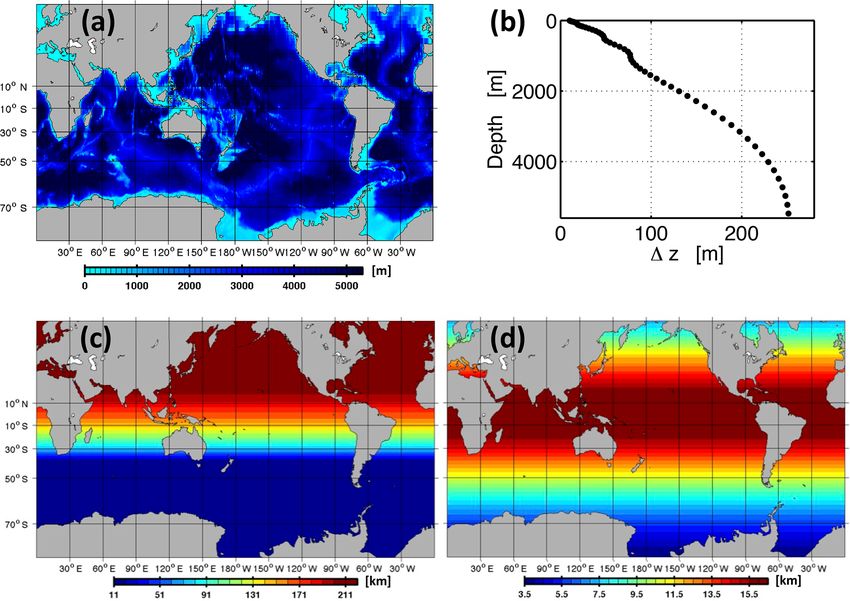
74                                                                                                         H. Dietze et al.: MOMSO 1.0

Figure 1. MOMSO model domain and spatial (finite difference) discretization. Panel (a) shows the model bathymetry. Panels (b), (c) and
(d) show the vertical, meridional and zonal resolutions, respectively. In total, there are 2400 × 482 × 55 grid boxes in zonal, meridional and
vertical directions, respectively.

all properties (such as temperature, salinity and biogeochem-            the model domain. This kept the respective oscillations in
ical variables) feature differing gradients, they are affected to        check. In addition, we added Laplacian viscosity at the exit
a differing degree by the spurious behavior of the advection             of the Drake Passage (Fig. 2).
scheme. Hence, even when using the same advection scheme
for all properties, the actual transport of properties is still in-
                                                                         2.3    Sea ice
consistent in that they are all affected by differing degrees
by spurious errors. This inconsistency can be larger than the
inconsistency introduced by switching from one advection                 The ocean component is coupled to a dynamical sea ice mod-
scheme to another. Note in this context that we do not apply             ule, the GFDL SIS. SIS uses elastic–viscous–plastic rhe-
an explicit horizontal background diffusivity other than the             ology adapted from Hunke and Dukowicz (1997). In the
contribution that is implicit to the advection scheme.                   standard version, the simulated sea ice impacts sea sur-
   Several decades into the spin-up, our configuration be-               face height. This led to a vicious cycle at some places
came unstable in coarsely resolved places where strong cur-              where sea ice attracted ever more sea ice, resulting in un-
rents met rough topography. This may well have been the                  realistic anomalies in sea surface height and finally in a
result of our very low choice of the Smagorinsky isotropic               numerical blow-up of the simulation. Because of the as-
viscosity (as reviewer 1 suspected). Our fix to the insta-               sociated computational cost, we did not investigate thor-
bility problem was to set an additional horizontal isotropic             oughly into this but – instead – switched to levitating sea
Laplacian viscosity of 600 m2 s−2 from 10◦ S to 50◦ N, of                ice by deleting line 1353 in the file ice_model.F90, which
1200 m2 s−2 above 50◦ N and 1800 m2 s−2 above 60◦ N out-                 reads Ice%p_surf(i,j) = Ice%p_surf(i,j) +
side the Southern Ocean towards the northern boundary of                 grav*x(i,j). Note that this is now also used, e.g., in Hor-
                                                                         doir et al. (2019), which is based on the Nucleus for Euro-

Geosci. Model Dev., 13, 71–97, 2020                                                             www.geosci-model-dev.net/13/71/2020/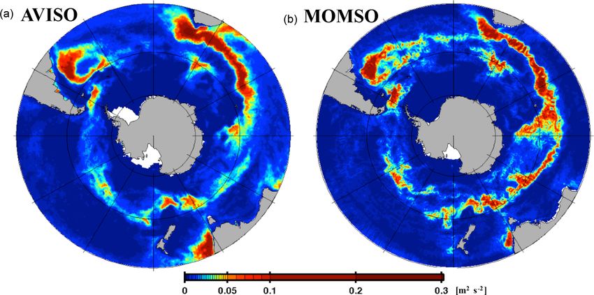
H. Dietze et al.: MOMSO 1.0                                                                                                           75

                                                                         macronutrients, two phytoplankton species, zooplankton and
                                                                         detritus) are hard to constrain with available observations al-
                                                                         ready (cf. Löptien and Dietze, 2015, 2017, 2019) – a diffi-
                                                                         culty that increases with the number of tracers. As a favorable
                                                                         side effect, the reduced number of prognostic tracers reduces
                                                                         the computational cost.

                                                                         2.5   Initial conditions and spin-up procedure

                                                                         The circulation model starts from rest (i.e., initial velocities
                                                                         are nil) with initial values for temperature and salinity taken
                                                                         from the World Ocean Atlas (WOA) 2009 (Locarnini et al.,
                                                                         2010; Antonov et al., 2009, respectively,). After 20 years of
                                                                         physics-only spin-up, the biogeochemical model is hooked
                                                                         on. In contrast to the physics, we do not use an observational
                                                                         product to initialize the prognostic variables of the biogeo-
                                                                         chemical model – also because the observations of dissolved
                                                                         iron are so sparse that Orr et al. (2017) suggest not to use
                                                                         them for model initialization. Instead, the initial conditions
                                                                         for the biogeochemical tracers are interpolated from the fully
                                                                         spun-up coarse-resolution configuration used by Dietze et al.
                                                                         (2017) (their “FMCD” simulation). This coarse-resolution
                                                                         configuration is, apart from the spatial discretization (and
                                                                         related parameters in the physical parameterizations of un-
                                                                         resolved processes), identical to the MOMSO configuration.
                                                                         A beneficial aspect of this spin-up is that it accelerates the
Figure 2. Close-up of MOMSO bathymetry in the Drake Passage.             equilibration of the carbon dynamics substantially compared
The color denotes depths in meters. The red rectangle denotes the        to initializing with an observational products. After a sub-
area where, from 3250 m down to the bottom, an additional Lapla-
                                                                         sequent 60-year spin-up with online biogeochemistry, the
cian horizontal viscosity of 1000 m2 s−2 is applied for stability rea-
sons.
                                                                         model allows already (as we will put forward in Sect. 4) for
                                                                         an investigation of circulation-driven decadal changes of the
                                                                         Southern Ocean carbon budget.
pean Modelling of the Ocean (NEMO) framework (Robinson
Hordoir, personal communication, 2019).                                  2.6   Boundary conditions and sponges

2.4   Biogeochemistry                                                    The boundaries towards the Arctic (i.e., the northern end of
                                                                         the model domain shown in Fig. 1) are closed (i.e., they
In our setup, the ocean–sea ice module is coupled to the                 are represented by solid and flat walls). Temperature and
BLING ecosystem model of Galbraith et al. (2010). BLING                  salinity are restored to climatological annual mean estimates
is a prognostic model that, in the basic version, explicitly re-         (Locarnini et al., 2010; Antonov et al., 2009) in so-called
solves only four biogeochemical tracers: dissolved inorganic             “sponge zones” located in the coarse-resolution domain. The
phosphorous, dissolved organic phosphorous, dissolved iron               sponge zones along with restoring timescales are shown in
and dissolved oxygen. Here, we use BLING in conjunction                  Fig. 3. The purpose of these sponges is to ensure realistic
with a carbon module that explicitly resolves dissolved inor-            deep-water characteristics even though Northern Hemisphere
ganic carbon and alkalinity as described, e.g., in Bernadello            deep-water formation processes are handicapped by the com-
et al. (2014).                                                           bination of coarse resolution with the absence of eddy param-
   The design idea behind the “reduced-tracer” model                     eterizations.
BLING is, on the one hand, to minimize the number of                        At the air–sea boundary, we apply climatological atmo-
prognostic tracers that are actually advected by the ocean-              spheric conditions taken from the Corrected Normal Year
circulation model and, on the other hand, to explicitly re-              Forcing (COREv2; Large and Yeager, 2004). In addition,
solve the most influential environmental processes that con-             we apply a surface salinity restoring to climatological val-
trol the net biotic carbon uptake (macro- and micronutrients             ues (Antonov et al., 2009) with a timescale of half a year
phosphorous and iron; oxygen which controls heterotrophic                throughout the model domain.
respiration). The rationale behind minimizing the number of                 Atmospheric CO2 concentrations are prescribed to a pre-
prognostic tracers is that even simple models (resolving only            industrial level of 278 ppmv. Thus, the simulated oceanic car-

www.geosci-model-dev.net/13/71/2020/                                                            Geosci. Model Dev., 13, 71–97, 2020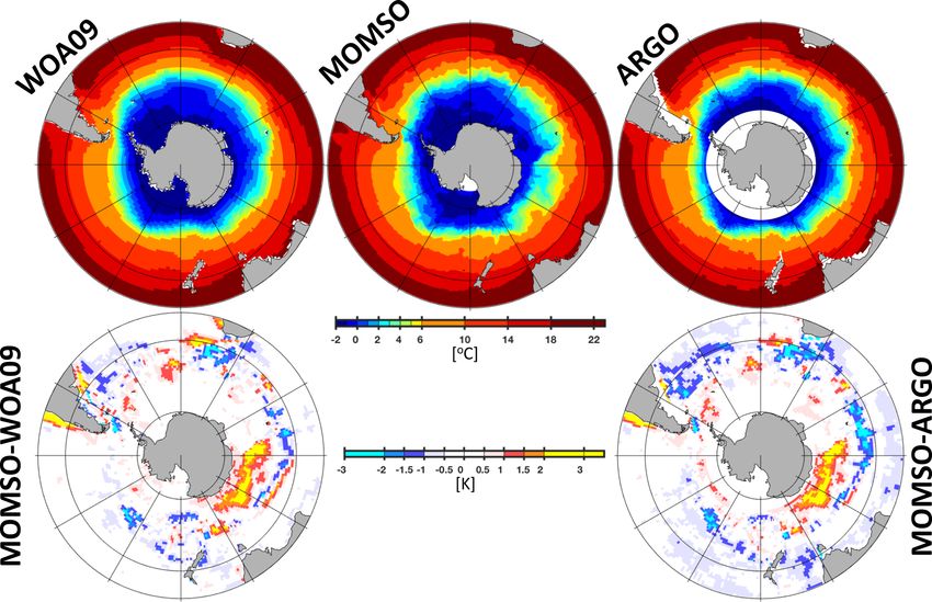
76                                                                                                 H. Dietze et al.: MOMSO 1.0

                                                                    gridded data product. Binning the observational data of sev-
                                                                    eral years or even decades into one product closes spatial data
                                                                    gaps, but then this blurs the referencing to an ever-changing
                                                                    (anthropogenically driven) system state. This problem is es-
                                                                    pecially pronounced in the Southern Ocean where in situ data
                                                                    acquisition is complicated by hostile environmental condi-
                                                                    tions.
                                                                       The climatological atmospheric boundary conditions
                                                                    which drive our ocean model are representative of the pe-
                                                                    riod 1958–2000. Climatological data products are typically
                                                                    biased in that they contain more recent observations, being
                                                                    the result of recent technological advances (such as the de-
Figure 3. MOMSO domains where temperature and salinity are re-      velopment of autonomous platforms). Hence, a model evalu-
stored to observed climatological values (Locarnini et al., 2010;   ation is not straightforward and it is difficult to define mean-
Antonov et al., 2009, respectively) throughout the water column.    ingful model–data misfit metrics. Further complexity comes
The red and blue patches denote e-folding restoring timescales of   from the fact that misfit metrics must be tailored to the actual
10 and 5 years, respectively.                                       application of the model in order to be meaningful.
                                                                       A potential application for the model configuration pre-
                                                                    sented here is to explore the role of mesoscale features, or ed-
bon is also referred to as “natural carbon”. Biogeochemical         dies, in determining the CO2 uptake of the Southern Ocean.
air–sea fluxes (of iron) are identical to the ones applied in       One hypothesis this model is set up to test is whether spa-
Galbraith et al. (2010) and Dietze et al. (2017).                   tially unresolved dynamics in IPCC-type coarse-resolution
   This paper refers to output from two simulations dubbed          models bias their oceanic carbon uptake sensitivity. In or-
REF and WIND. Both simulations share the same 80-year               der to come to a meaningful conclusion on this, our high-
spin-up described in Sect. 2.5. WIND branches off from              resolution model has to perform with a fidelity similar or
REF during the nominal year 1980 and is exposed to ever-            superior to that of IPCC-type coarse-resolution models. In
increasing wind speeds south of 40◦ S. The increase is linear       the following, we list and explain our choice of model as-
at a rate of 14 % in 50 years, consistent with results from         sessments which we deem relevant in this respect. Wherever
a reanalysis of the period 1958 to 2007 (Lovenduski et al.,         applicable, we will follow the approach taken by Sallée et al.
2013). The rationale behind presenting results from the sen-        (2013a, b), who assessed the performance of CMIP5 models,
sitivity experiment WIND in this model description paper is         and Russell et al. (2018), who suggested evaluation metrics
that they serve as a reference point against which the remain-      for the Southern Ocean in coupled climate models and Earth
ing model drift in REF (which is there since we cannot af-          system models.
ford thousands of years of spin-up) can be compared. Based             Please note that we refrain from using state estimates
on this comparison, Sect. 4 sketches – very briefly – research      based on data assimilation such as the Biogeochemical
questions that may be tackled with MOMSO.                           Southern Ocean State Estimate (B-SOSE) (Verdy and Ma-
   IO-related hardware problems caused data loss such that          zloff, 2017) for biogeochemical parameters. On the one hand,
REF covers the period from 1980 to 2024, while WIND cov-            these state estimates are especially useful in the Southern
ers 1980 to 2022 only.                                              Ocean, where observational data are particularly sparse. On
   Please note that a comprehensive analysis of the sensitiv-       the other hand, these estimates rely – especially when ob-
ity experiment WIND is beyond the scope of this model de-           servational data are sparse – on the realism of the underly-
scription paper. Our major aim here is to show that REF is          ing ocean-circulation biogeochemical model framework. In
sufficiently equilibrated so that trends affected by decadal-       the case of B-SOSE, the underlying model framework is so
scale changes in winds can clearly be distinguished against         similar to our model configuration (high-resolution ocean-
the background trend that is still persistent.                      circulation model coupled to the biogeochemical model of
                                                                    Galbraith et al., 2010) that we essentially would assess the
                                                                    benefit of the assimilation scheme in fitting observational
3    Results                                                        data rather than assessing our model configuration.
                                                                       The model–data comparison is divided into the following
In the following, we evaluate our model (simulation REF) by         subsections:
comparing our climatological results from the nominal years
1980–2024 to observational data. One problem is the tradeoff          – Ocean circulation (Sect. 3.1), e.g., affects the transport
between data coverage and the length of the period the data             of carbon-rich deepwater to the surface, shapes the lo-
are representative of. For any given year, the data coverage            cations of fronts and constitutes a major pathway for
is insufficient to compile a comprehensive three-dimensional            nutrients that are essential for phytoplankton growth.

Geosci. Model Dev., 13, 71–97, 2020                                                     www.geosci-model-dev.net/13/71/2020/
H. Dietze et al.: MOMSO 1.0                                                                                                77

    For the evaluation of surface currents, we use exem-           temperature (SST) can be directly observed from space
    plary snapshots showcasing main circulation paths and          and therefore is available in an unrivaled (compared to
    spatial variability, along with climatological sea surface     in situ measured properties) spatial and temporal res-
    height which is indicative of the barotropic circulation.      olution. In contrast, temperature observations at depth
    More quantitative measures of transport characteristics        are unfortunately much sparser even though deep tem-
    are provided for the ACC (Drake Passage transport) and         peratures determine important processes, e.g., for basal
    the Southern Ocean meridional overturning circulation.         melting, and thus are related to the formation rate of
    Further, we assess the strength of the cyclonic Ross and       Antarctic Bottom Water (AABW). AABW formation,
    Weddell polar gyres which are formed by interactions           in turn, affects the solubility and biotic pump of carbon.
    between the ACC and the Antarctic continental shelf.
    Special emphasis is here on the larger Weddell Gyre.         – Salinity (Sect. 3.5) is related to the density of seawa-
    This gyre entrains heat and salt from the ACC and car-         ter. Saltening by brine rejection can cause convection;
    ries them to the Antarctic continental shelves, where          meltwater, on the other hand, can form buoyant lenses,
    deep and bottom waters are produced and thus estab-            thus increasing the local stability of the water column
    lish an intermittent connection between the atmosphere         which prevents vertical mixing. Spatial salinity gradi-
    (surface ocean) and the deep oceanic carbon (nutrient)         ents are associated with geostrophic circulation (if they
    pool.                                                          are not temperature compensated). Vertical salinity gra-
                                                                   dients affect the stability of the water column and pre-
  – Eddy kinetic energy (EKE; Sect. 3.2) is an important           condition vertical mixing.
    measure for the mesoscale activity and thus a key proxy
    for realistically reproduced eddy dynamics. At the sur-      – Sea ice (Sect. 3.6) caps the direct exchange between at-
    face, the EKE can be derived from the variability of the       mosphere and ocean and thus controls the air–sea gas
    sea surface height (SSH), a measure that can be directly       exchange of CO2 . It also modulates the air–sea buoy-
    observed from space by satellite altimetry.                    ancy forcing by, e.g., insulating the surface from heat
                                                                   loss or by brine rejection during ice formation. Further,
  – Surface mixed layer depth (MLD; Sect. 3.3) is deter-           it shields the surface water from solar irradiance and
    mined by (1) the stability of the water column (i.e.,          hampers the assimilation of CO2 by autotrophic plank-
    the vertical density gradient), (2) wind-induced turbu-        ton.
    lence which provides energy for eroding the stability
    and thereby deepens the MLD and (3) air–sea buoy-            – Nutrients (Sect. 3.7) are essential to the growth of au-
    ancy fluxes which can, depending on their sign, increase       totrophic plankton, and their availability exerts a ma-
    or decrease the stability of the water column and thus         jor control on the biological pump. The most impor-
    shallow or deepen the MLD. The MLD is an impor-                tant macronutrient is bioavailable phosphorous (such
    tant concept or metric because it locates that fraction        as phosphate, PO4 ), because its availability is essential
    of the upper water column that is in direct contact with       to all phytoplankton (and cyanobacteria). The distribu-
    the atmosphere and sets air–sea gradients of tempera-          tion of PO4 is determined by the interplay between the
    ture and partial pressure of gases (such as carbon diox-       ocean circulation (transporting PO4 dissolved in sea-
    ide or oxygen). Further, changes in MLD modulate the           water) and marine biota which utilize phosphorous to
    level of average light levels experienced by phytoplank-       build biomass (typically at the surface) and release PO4
    ton: deep MLDs define conditions where phytoplankton           in the course of degradation of organic material (typ-
    spend more time mixed downwards away from the sun-             ically at depth). In addition, we assess simulated iron
    lit surface. This reduces phytoplankton growth and as-         concentrations since the Southern Ocean is well known
    sociated biotic carbon uptake. Antagonistic to this light      for being a site where iron is limiting the growth of au-
    deprivation, however, deepening MLDs are typically as-         totrophs (e.g., Boyd and Ellwood, 2010). Further, in or-
    sociated with transports of nutrients (essential for phy-      der to guide the interpretation of simulated PO4 concen-
    toplankton) from depth to the sunlit nutrient-depleted         trations at depth, we include a meridional section of dis-
    surface.                                                       solved oxygen in this section: oxygen is reset to values
                                                                   close to saturation at the surface, while its sinks in the
  – Temperatures (Sect. 3.4), which influence the rate of bi-      interior are typically assumed to be linearly linked to in-
    ological turnover, affect the solubility pump of carbon        terior sources of PO4 (which is not reset at the surface).
    and the density of seawater. Cooling typically results in      Hence, cases where biases in simulated PO4 concentra-
    a reduction of buoyancy and causes convection. Spatial         tions are inconsistent with biases in simulated oxygen
    temperature gradients are associated with geostrophic          concentrations contain information on what exactly is
    circulation (if they are not salinity compensated). Verti-     the cause for the simulated biases within the interplay
    cal temperature gradients affect the stability of the wa-      of ocean circulation and biogeochemistry.
    ter and precondition vertical mixing. The sea surface

www.geosci-model-dev.net/13/71/2020/                                                  Geosci. Model Dev., 13, 71–97, 2020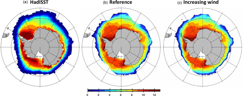
78                                                                                                    H. Dietze et al.: MOMSO 1.0

Figure 4. Climatological mean sea surface height in units of centimeters. Panel (a) shows a 1993 to 1998 climatological average observed
from space (Maps of Absolute Geostrophic Current (MADT) Aviso data). Panel (b) shows a 6-year average (nominal years 1993 to 1998)
simulated with the reference simulation. The white patches in panels (a) and (b) indicate missing data and (spurious) model land mask,
respectively.

3.1   Ocean circulation                                               (Fig. 6), which is located right in the transition zone from
                                                                      very high to very coarse resolution (see Fig. 1c), highlights
Figure 4 shows simulated climatological SSH, along with an            that the realism of simulated patterns is sustained right up
estimate based on observations from space (Maps of Abso-              into the transition to coarser, non-eddy-resolving resolution.
lute Geostrophic Current (MADT) Aviso). The model cap-                   Figure 7 features the simulated transport through the
tures the main features of the global barotropic circulation,         Drake Passage. (Here, we refer to the reference simulation
even in the coarsely resolved domain north of 40◦ S, such as          only; simulation WIND is discussed in Sect. 4.) The sim-
in the subtropical gyres in both hemispheres north and south          ulated Drake Passage transport averages to 99 Sv (nominal
of the Equator (positive SSH anomalies) and in the subpolar           years 1980–2023). This is biased low compared to available
gyres around 50 and 60◦ N in the Pacific and Atlantic (neg-           observational estimates that range from 110 to 170 Sv (With-
ative SSH anomalies), respectively. Further, as indicated by          worth, 1983 for 1979; Cunningham et al., 2003 for 1993–
the transition from yellow to blue in the Southern Ocean in           2000; Chidichima et al., 2014 for 2007–2011). Note that sim-
Fig. 4, the model reproduces the northern boundary of the             ilar biases have been reported in other high-resolution con-
Antarctic Circumpolar Current (ACC), also referred to as the          figurations and may, according to Dufour et al. (2015), be
northern edge of the Subantarctic Front (SAF).                        related to a deficient representation of the overflow of dense
   A quantitative numerical comparison of observed (Aviso)            waters formed along the Antarctic coasts. If so, the ACC bias
and simulated climatologic surface speeds yields a spatial            may well be endemic to z-level models which struggle to rep-
correlation of 0.6 in the high-resolution domain south of             resent complex topography (in comparison to more elaborate
40◦ N. The spatial variance in the speed of simulated sur-            numerical approaches, e.g., finite elements). A comprehen-
face currents is typically 30 % higher than the observational         sive investigation is beyond the scope of this paper. But, still,
estimate and the respective simulated mean is 20 % higher             the problem is an intriguing one – especially since, histori-
than in the observations. Apparently, a (yet-to-be-quantified)        cally, (coarse-resolution) models started out from an oppos-
fraction of this misfit is attributable to errors in the estimates    ing bias dubbed “Hidaka’s dilemma” (Hidaka and Tsuchiya,
from space (cf. Fratantoni, 2001).                                    1953), where an excessive ACC transport could only by ap-
   Figure 5 shows exemplary snapshots of the surface veloci-          plication of unrealistically high friction be fenced into real-
ties as observed from space (Fig. 5a, MADT Aviso) and sim-            istic bounds.
ulated (Fig. 5b, MOMSO). The boundary conditions of the                  In terms of Eulerian meridional overturning in the South-
model are not identical to the atmospheric boundary condi-            ern Ocean, our model values are consistent with the South-
tions on that specific day, and the highly non-linear charac-         ern Ocean state estimate of Mazloff et al. (2010): Mazloff
teristics of eddy dynamics render an “eddy-to-eddy” similar-          et al. (2010) find a surface meridional overturning cell across
ity without data assimilation impossible. So the purpose of           32◦ S of 12 ± 12 Sv and an abyssal cell of 13 ± 6 Sv. We find
Fig. 5 is to demonstrate the similarity of patterns and the ma-       a climatological mean value for the upper cell of 12 ± 4 and
jor transport pathways in the high-resolution domain south            8 ± 3 Sv for the lower cell. Please note that more elaborate
of 40◦ N. The close-up into the Agulhas retroflection zone            measures such as the physically more meaningful overturn-

Geosci. Model Dev., 13, 71–97, 2020                                                         www.geosci-model-dev.net/13/71/2020/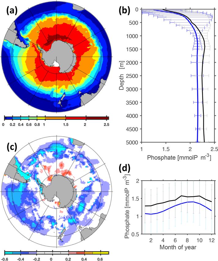
H. Dietze et al.: MOMSO 1.0                                                                                                                79

Figure 5. Magnitude of surface velocities. Panels (a) and (b) show typical snapshots as observed from space (Aviso, 3 May 1995) and as
simulated (MOMSO, 3 May of nominal year 2020), respectively.

                                                                        Figure 7. Simulated volume transport of the Antarctic Circumpo-
                                                                        lar Current through the Drake Passage in units of 106 m3 s−1 . The
                                                                        black (red) line refers to the reference (increasing wind) simulation.

                                                                        ing calculated on density coordinates or its approximation
                                                                        given by the residual mean streamfunction (cf. McIntosh and
                                                                        McDougall, 1996; Viebahn and Eden, 2010) are beyond the
                                                                        scope of this paper (which is intended to serve as a model
                                                                        description only).
                                                                           In terms of transports of the Weddell and Ross gyres, our
Figure 6. Magnitude of surface velocities. Panels (a) and (b) show      simulation is slightly biased high. In the Weddell Gyre, we
typical snapshots as observed from space (Aviso, 3 May 1995) and        simulate 70 Sv, while published estimates range from 40 ±
as simulated (MOMSO, 3 May of nominal year 2020), respectively.         8 Sv (Southern Ocean state estimate; Mazloff et al., 2010) to
This is a close-up from Fig. 5, focusing on those latitudes where the
                                                                        56 ± 10 Sv (recent SODA estimate Yongliang et al., 2016),
meridional resolution transitions from eddy permitting in the south
to eddy prohibiting in the north.
                                                                        55.9 ± 9.8 and 61–66 Sv (Schröder and Fahrbach, 1999). In
                                                                        the Ross Gyre, we simulate 35 Sv, while published estimates
                                                                        range from 20±5 Sv (Mazloff et al., 2010) to 15–30 Sv (Chu
                                                                        and Fan, 2007) and 37 ± 6 Sv (Yongliang et al., 2016).

www.geosci-model-dev.net/13/71/2020/                                                              Geosci. Model Dev., 13, 71–97, 2020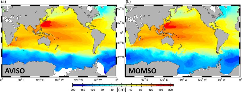
80                                                                                                         H. Dietze et al.: MOMSO 1.0

Figure 8. Eddy kinetic energy. Panel (a) is calculated from 1993–1998 satellite altimetry (Maps of Sea Level Anomalies and Geostrophic
Velocity Anomalies (MSLA) Aviso data) observations. Panel (b) corresponds to a 6-year average (nominal years 1993 to 1998) calculated
from daily averaged surface velocities from the reference simulation. The white patches in the left and right panels indicate missing data and
(spurious) model land mask, respectively.

3.2   Eddy kinetic energy and sea surface height

Figure 8 shows that the simulated climatological EKE re-
produces the amplitudes and spatial pattern observed from
space (Maps of Sea Level Anomalies and Geostrophic Veloc-
ity Anomalies (MSLA) Aviso data) as can be expected from
high-resolution configurations (e.g., Delworth et al., 2012;
Barnier et al., 2006). This applies especially in the high-
resolution region south of 40◦ S, where typical deviations in
simulated EKE are rather small (< 0.03 m2 s−2 ) compared
to the maximum values found in the ACC (> 0.3 m2 s−2 ; cf.
Fig. 9). The correlation coefficient between simulated and
observed EKE patterns is 0.7. The simulated EKE features
7 % more spatial variance and an average of 8 % more en-
ergy within the high-resolution domain south of 40◦ S. By
averaging all simulated values with their immediate spatial
neighbors two times consecutively, the simulated variance
levels become more similar to observed values and the re-
spective correlation increases to 0.71. We interpret this as an
indication that the model resolution is higher than the effec-
tive spatial resolution of the MSLA Aviso data. This may also
explain why simulated EKE amplitudes are generally higher                Figure 9. Difference between observed and simulated eddy kinetic
                                                                         energy. Blue colors denote regions where the observed levels cal-
than estimates from space (cf. Fratantoni, 2001).
                                                                         culated from 1993–1998 satellite altimetry (MSLA Aviso data) ob-
   We conclude that we found no evidence of an underesti-                servations are lower than simulated levels. The region outside the
mation of simulated mesoscale activity. This, in turn, implies           high-resolution nest (north of 40◦ S) is masked by a white patch.
that our combination of spatial resolution and (parameteriza-
tion of) friction in the Southern Ocean is suitable to allow for
investigations into eddy-driven processes.                               3.3    Surface mixed layer depth

                                                                         MLD is a concept that locates that fraction of the up-
                                                                         per water column that is well mixed. MLD is typically
                                                                         derived from vertical profiles of temperature and salinity

Geosci. Model Dev., 13, 71–97, 2020                                                             www.geosci-model-dev.net/13/71/2020/
H. Dietze et al.: MOMSO 1.0 81
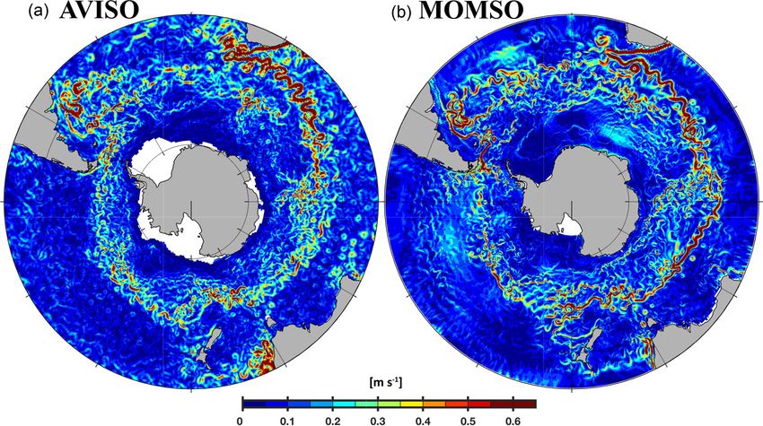
Figure 10. Surface mixed layer depth in units of meters. The upper (lower) line refers to austral winter (summer). The columns refer to
(observed) CARS 2009 climatology based on Condie and Dunn (2006), Argo Al. and Argo Thresh. computed from (observed) profiles of
Argo floats using two different methods by Holte et al. (2017) and our simulation (MOMSO). White patches in Argo Al. and Argo Thresh.
denote missing data.
rather than from direct measurements of mixing intensity both winter and summer – irrespective of algorithm). Argo
(i.e., turbulence). As a consequence, algorithms calculat- Thresh. is closest to our simulated pattern (fourth row in
ing MLDs struggle with distinguishing between identifying Fig. 10), and we find correlations of 0.5 and 0.6 in summer
actively mixed layers and those which have been actively and winter, respectively.
mixed in the past but are no longer fed by energy fuel- In summary (cf. winter statistics in Fig. 11), we find that
ing actual turbulence and associated mixing. The first three the average of variance in simulated MLDs is higher than in
columns of Fig. 10 provide a comparison between contem- the observations and that the differences in correlation from
porary (in the sense that they are still used in current peer- one MLD product to another are comparable to our model–
reviewed literature) databases and algorithms to compute observation misfit. In terms of bias, we find that our sim-
MLD: CARS 2009 distributed by CSIRO http://www.marine. ulated winter MLD is, on average, 18 m deeper than Argo
csiro.au/~dunn/cars2009/ (last access: 1 November 2019) Thresh. This is a major improvement compared to (coarse-
and introduced by Condie and Dunn (2006) is predominantly resolution and fully coupled) CMIP5 models which feature
based on historical conductivity–temperature–depth (CTD) similar correlations but winter mixed layer depths biased low
observations, while both Argo Al. and Argo Thresh. are by typically 50–100 m (Sallée et al., 2013a, their Fig. 4a).
based on observations from Argo floats. The difference be-
tween Argo Al. and Argo Thresh. is the algorithm used to de- 3.4 Temperature
rive MLDs in Holte et al. (2017). We find a high correlation
between the different algorithms Argo Al. and Argo Thresh.
Figure 12 shows a comparison of the simulated SST
in the region south of 40◦ S (0.98 and 0.91 in summer and
with WOA09 (Locarnini et al., 2010) and Argo-float-based
winter, respectively). The correlation from one database to
(Roemmich and Gilson, 2009) observations. The overall pat-
another (i.e., Argo vs. CARS 2009) is much lower (≈ 0.7 for
tern is well reproduced – an exception being a local high bias
www.geosci-model-dev.net/13/71/2020/ Geosci. Model Dev., 13, 71–97, 202082 H. Dietze et al.: MOMSO 1.0
bias of an ensemble mean bias of 3.5 ◦ C in CMIP5 mod-
els (Sallée et al., 2013b).
– Intermediate water (IW) is a denser type of MW which
ventilates the thermocline and is sequestered away from
the atmosphere longer than MW because it protrudes
deeper into the water column. MOMSO’s IW is biased
warm by ≈ 1.1 ◦ C (Fig. 15), which compares favorably
against the 3.5 ◦ C warm bias in CMIP5 models (Sallée
et al., 2013b).
– During its formation at the surface, circumpolar deep
water (CDW) taps into the abyssal waters rich in nat-
ural carbon. Hence, it plays a key role for the oceanic
sequestration of natural carbon dioxide (e.g., Le Quéré
et al., 2009). MOMSO overestimates the CDW tem-
perature by ≈ 1 ◦ C. This is substantially more than the
0.4 ◦ C overestimation of the CMIP5 ensemble mean but
still within the envelope of the ensemble, which peaks
at an overestimation of 1.5 ◦ C (Sallée et al., 2013b).
Figure 11. Taylor diagram of surface mixed layer depth in austral – MOMSO overestimates Antarctic Bottom Water (BW)
winter referred to as Argo Thresh. observational data compiled by temperatures by 1 ◦ C, while the CMIP5 ensemble mean
Holte et al. (2017). The units for the standard deviation and root compares more favorably with an underestimation of
mean square deviations are meters. Argo Al. refers also to obser- only 0.4 ◦ C. These biases are consistent with MOMSO
vational data compiled by Holte et al. (2017) but based on a differ- featuring too much sea ice coverage which caps the
ent algorithm. CARS 2009 is a climatology based on observations ocean from the cooling atmosphere (cf. Sect. 3.6). Like-
compiled by Condie and Dunn (2006), and MOMSO refers to the wise, CMIP5 models tend to underestimate sea ice cov-
high-resolution reference simulation presented in this study. erage (Turner et al., 2013), which may overly expose the
ocean to the cooling atmosphere and thereby cause the
of about 3 ◦ C close to the Antarctic coast (between 120 and respective cold bias in BW temperature.
160◦ E). Averaged over the Southern Ocean (Fig. 13), the
simulated SSTs are within the observational range (although 3.5 Salinity
at the lower edge) of the years 1960 to 2010 (Fig. 14 calcu-
lated from HadISST; Rayner et al., 2003). Figure 16 shows a comparison of the simulated climatolog-
Figure 15 summarizes the fidelity of simulated tempera- ical mean sea surface salinity (SSS) with three observation-
tures in the interior. Following Sallée et al. (2013b) and their based products (WOA09, Antonov et al., 2009; Argo, Roem-
density-based water mass criteria, we discuss the five major mich and Gilson, 2009; and SMOS, Köhler et al., 2015).
water masses (subtropical water, mode water, intermediate Within the spatially highly resolved Southern Ocean, the
water, circumpolar deep water, bottom water) separately: simulated sea surface salinity is in good agreement with
– With subtropical water (TW), MOMSO features a slight the observations. Towards the north, where the resolution
cold bias at the surface (less than 0.5 ◦ C) and a warm coarsens, the model fidelity disintegrates; particularly in the
bias of ≈ 1 ◦ C in the interior (Fig. 15). This is appar- Atlantic and Indian sectors, the model is biased low.
ently very good when compared against the 2.7◦ warm Averaged over the Southern Ocean, the simulated SSS
bias in the CMIP5 models (Sallée et al., 2013b). There is biased low (compare reference in Fig. 17) compared to
are, however, indications that the 2.7◦ bias is a con- recent observational estimates during 2005–2017 (Fig. 18).
sequence of biased air–sea heat fluxes in the Southern Figure 17 suggests that increasing winds can increase simu-
Hemisphere in the coupled models rather than the con- lated SSSs up to observed values. This could be interpreted
sequence of an unrealistic oceanic circulation. as a mismatch between the climatological forcing (represent-
ing the years 1958–2000) and the observation period. (Please
– The subduction of surface waters is dominated by mode note that a comprehensive analysis is beyond the scope of
water (MW) in the Southern Ocean. Hence, MW is an this model description paper.) Figure 17 suggests further that
important agent in sequestering anthropogenic carbon the surface salinity restoration (cf. Sect. 2.6) is weak enough
away from the atmosphere. MOMSO’s MW is too warm to allow for substantial SSS dynamics in response to, e.g.,
by ≈ 1 ◦ C, which compares favorably to the much larger increasing winds.
Geosci. Model Dev., 13, 71–97, 2020 www.geosci-model-dev.net/13/71/2020/H. Dietze et al.: MOMSO 1.0 83
Figure 12. Climatological mean sea surface temperature. WOA09 and Argo (2004–2017 period) refer to observations compiled by Locarnini
et al. (2010) and Roemmich and Gilson (2009), respectively. MOMSO refers to an average over the nominal 1993–1998 period of the
reference simulation. The upper (lower) panels show sea surface temperature (differences).
Figure 13. Simulated sea surface temperature averaged over the Figure 14. Observational estimate of annual mean sea surface tem-
Southern Ocean (i.e., south of 40◦ S). The black (red) line refers peratures south of 40◦ S calculated from HadISST (Rayner et al.,
to the reference (increasing wind) simulation. 2003).
Figure 19 summarizes the fidelity of simulated salinities in
the interior. Following Sallée et al. (2013b) and their density- els which is – in contrast to MOMSO – enhanced, in
based water mass criteria, we discuss the five major water terms of biasing the density towards smaller values, by
masses (subtropical water, mode water, intermediate water, a 2.7 ◦ C warm bias.
circumpolar deep water, bottom water) separately:
– For TW, MOMSO is biased low by 0.5 at the surface, – For MW, MOMSO is biased low by 0.1 at the surface
and this makes the simulated TW too light in compari- and high by 0.1 in the interior. This is in line with the
son with WOA09 observations. Sallée et al. (2013b) find overall poor performance of CMIP5 models in repre-
a smaller ensemble mean bias of 0.2 in the CMIP5 mod- senting the MW (Sallée et al., 2013b). Coincidentally,
www.geosci-model-dev.net/13/71/2020/ Geosci. Model Dev., 13, 71–97, 202084 H. Dietze et al.: MOMSO 1.0
3.6 Sea ice
Figure 20 shows a comparison of the simulated number of
sea-ice-covered months per year with an observation esti-
mate (HadISST; Rayner et al., 2003). Overall, the agreement
is good, with the following two exceptions: (1) in the Weddell
and Ross seas, the period of ice coverage is underestimated
by 2 months. We speculate that this triggers elevated air–sea
momentum fluxes and, eventually, biases the respective gyre
strengths high (cf. Sect. 3.1). (2) Overall, the simulated ice
extent is biased high (compare Fig. 21, black line, to Fig. 22).
Following Russell et al. (2018) we compare the data, in ad-
dition, against the fractional sea ice coverage obtained from
the National Snow and Ice Data Center (NSIDC; ftp://sidads.
colorado.edu/pub/DATASETS/NOAA/G02202_v2/, last ac-
Figure 15. Zonally averaged meridional section of temperature in
units of ◦ C. Panel (a) refers to simulated concentrations averaged cess: 1 September 2019). The comparison in Fig. 23 confirms
over the nominal 1993–1998 period of the reference simulation; the impression that the model overestimates sea ice coverage.
(b) refers to observed climatological values (WOA09); (c) refers Figure 21 suggests that increasing the wind speeds to levels
to the difference between simulated and observed values, with blue that are more representative of the time period of observa-
colors denoting simulated temperatures that are biased low. The tions shown in Fig. 22 alleviates this model bias. In addition,
thick black, red, cyan, blue and green contours refer to mean densi- Fig. 23 reveals that the model bias features a seasonality with
ties (Sallée et al., 2013b, their Table 2) of subtropical water, mode underestimation in January until March and an overestima-
water, intermediate water, circumpolar deep water and bottom wa- tion of ice coverage from May to December. Ranked against
ter, respectively. the current generation of IPCC models, MOMSO fits well
into the envelope of the ensemble reported by Turner et al.
(2013).
the ensemble mean over all the CMIP5 models averages
to a very small fresh bias of 0.02. 3.7 Nutrients
– For IW, MOMSO is, again, biased low by 0.1 at the sur- Simulated Southern Ocean PO4 surface concentrations are
face and high by 0.1 in the interior. This dampens the biased low, locally down to 0.6 mmol P m−3 (Fig. 24a, c).
equatorward protruding of IW’s salinity-minimum sig- The reason is not straightforward to identify because it could
nature. Compared against the high bias of only 0.008 be associated with a deficient physical module, a deficient
in the ensemble mean over all the CMIP5 models, biogeochemical module or both. In the following, we will
MOMSO’s bias appears substantial. Compared, how- present an indication that the problem is associated with a
ever, against individual CMIP5 models whose charac- deficient formulation of iron limitation, argue why the for-
teristics vary widely (Sallée et al., 2013b), MOMSO is mulation of light limitation is unlikely to be the main prob-
comparable (i.e., within the envelope spanned by the lem and put the model–data misfit into perspective.
CMIP5 models). Southern Ocean uptake of PO4 in the sunlit surface by au-
totrophic phytoplankton is known to be limited by the avail-
– For CDW, MOMSO is biased high by 0.07 south of ability of light and the availability of the micronutrient iron.
75 ◦ S at the surface and less than 0.02 equatorwards. Figure 25 features a comparison of simulated iron concentra-
These small biases are well within the range set by the tions with observations. Even though the spatial and tempo-
CMIP5 models and of the same order of magnitude as ral coverage of iron measurements is still sparse, the emerg-
the bias of 0.02 of the CMIP5 ensemble. ing pattern is one where the simulated biotic iron drawdown
at the surface appears to be too strong. Surface iron con-
– For BW, MOMSO’s bias is identical to the high bias of centrations are biased low, just like the PO4 concentrations,
0.06 in the CMIP5 ensemble mean (Sallée et al., 2013b) and they appear so throughout an annual cycle. Such de-
and much better than the up-to-0.5 biases of many indi- ficient model behavior can be caused by insufficient throt-
vidual CMIP5 members. The bias is consistent with the tling of phytoplankton growth by both iron and light limi-
bias in sea ice: an overestimated ice production releases tation. Looking closer at seasonal model–data misfits, how-
too much brine and shields the ocean from atmospheric ever, suggests that a deficient iron limitation is more likely
cooling. This drives spuriously elevated salinities and to be the cause: the dependency of growth (and associated
temperatures. micro- and macronutrient drawdown at the surface) is known
to be a highly non-linear function of environmental drivers.
Geosci. Model Dev., 13, 71–97, 2020 www.geosci-model-dev.net/13/71/2020/H. Dietze et al.: MOMSO 1.0 85 Figure 16. Climatological mean sea surface salinity in psu. WOA09, Argo (2004–2017 period) and SMOS in the upper panels refer to observations compiled by Antonov et al. (2009), Roemmich and Gilson (2009) and Köhler et al. (2015), respectively. MOMSO in the lower panel refers to an average over the nominal 1993–1998 period of the reference simulation. MOMSO-WOA09 and MOMSO-Argo refer to sea surface salinity differences between the reference simulation and respective observations. Figure 17. Simulated sea surface salinity averaged over the South- Figure 18. Observed sea surface salinity averaged over the Southern ern Ocean (i.e., south of 40◦ S) for the nominal years 1980–2024. Ocean (i.e., south of 40◦ S) based on Argo data (Roemmich and The black (red) line refers to the reference (increasing wind) simu- Gilson, 2009). lation. We find that the bias in surface PO4 concentrations is almost the result of non-linear forcing modulating a deficient non- constant over the course of a seasonal cycle (Fig. 24d), even linear formulation of PO4 limitation such that the model bias though the photosynthetically available radiation varies dra- stays constant over a wide range of environmental conditions matically from season to season in the respective latitudes (here seasons). But this is unlikely. Looking into the seasonal (also because radiation experienced by phytoplankton cells bias of simulated iron concentrations (Fig. 25d), we find that dispersed in surface waters is a function of the seasonally it varies substantially from season to season compared to the varying surface mixed layer depth). By chance, this could be respective PO4 variability (Fig. 24d) – just as is expected www.geosci-model-dev.net/13/71/2020/ Geosci. Model Dev., 13, 71–97, 2020
You can also read