Multi-source global wetland maps combining surface water imagery and groundwater constraints
←
→
Page content transcription
If your browser does not render page correctly, please read the page content below
Earth Syst. Sci. Data, 11, 189–220, 2019
https://doi.org/10.5194/essd-11-189-2019
© Author(s) 2019. This work is distributed under
the Creative Commons Attribution 4.0 License.

          Multi-source global wetland maps combining surface
               water imagery and groundwater constraints
                                    Ardalan Tootchi, Anne Jost, and Agnès Ducharne
             Sorbonne Université, CNRS, EPHE, Milieux environnementaux, transferts et interaction dans les
                                  hydrosystèmes et les sols, Metis, 75005 Paris, France
                          Correspondence: Ardalan Tootchi (ardalan.tootchifatidehi@upmc.fr)

                                   Received: 26 July 2018 – Discussion started: 22 August 2018
                       Revised: 13 December 2018 – Accepted: 9 January 2019 – Published: 6 February 2019

      Abstract. Many maps of open water and wetlands have been developed based on three main methods: (i) com-
      piling national and regional wetland surveys, (ii) identifying inundated areas via satellite imagery and (iii) de-
      lineating wetlands as shallow water table areas based on groundwater modeling. However, the resulting global
      wetland extents vary from 3 % to 21 % of the land surface area because of inconsistencies in wetland defini-
      tions and limitations in observation or modeling systems. To reconcile these differences, we propose composite
      wetland (CW) maps, combining two classes of wetlands: (1) regularly flooded wetlands (RFWs) obtained by
      overlapping selected open-water and inundation datasets; and (2) groundwater-driven wetlands (GDWs) derived
      from groundwater modeling (either direct or simplified using several variants of the topographic index). Wet-
      lands are statically defined as areas with persistent near-saturated soil surfaces because of regular flooding or
      shallow groundwater, disregarding most human alterations (potential wetlands). Seven CW maps were gener-
      ated at 15 arcsec resolution (ca. 500 m at the Equator) using geographic information system (GIS) tools and by
      combining one RFW and different GDW maps. To validate this approach, these CW maps were compared with
      existing wetland datasets at the global and regional scales. The spatial patterns were decently captured, but the
      wetland extents were difficult to assess compared to the dispersion of the validation datasets. Compared with
      the only regional dataset encompassing both GDWs and RFWs, over France, the CW maps performed well and
      better than all other considered global wetland datasets. Two CW maps, showing the best overall match with the
      available evaluation datasets, were eventually selected. These maps provided global wetland extents of 27.5 and
      29 million km2 , i.e., 21.1 % and 21.6 % of the global land area, which are among the highest values in the litera-
      ture and are in line with recent estimates also recognizing the contribution of GDWs. This wetland class covers
      15 % of the global land area compared with 9.7 % for RFW (with an overlap of ca. 3.4 %), including wetlands
      under canopy and/or cloud cover, leading to high wetland densities in the tropics and small scattered wetlands
      that cover less than 5 % of land but are highly important for hydrological and ecological functioning in temperate
      to arid areas. By distinguishing the RFWs and GDWs based globally on uniform principles, the proposed dataset
      might be useful for large-scale land surface modeling (hydrological, ecological and biogeochemical modeling)
      and environmental planning. The dataset consisting of the two selected CW maps and the contributing GDW and
      RFW maps is available from PANGAEA at https://doi.org/10.1594/PANGAEA.892657 (Tootchi et al., 2018).

Published by Copernicus Publications.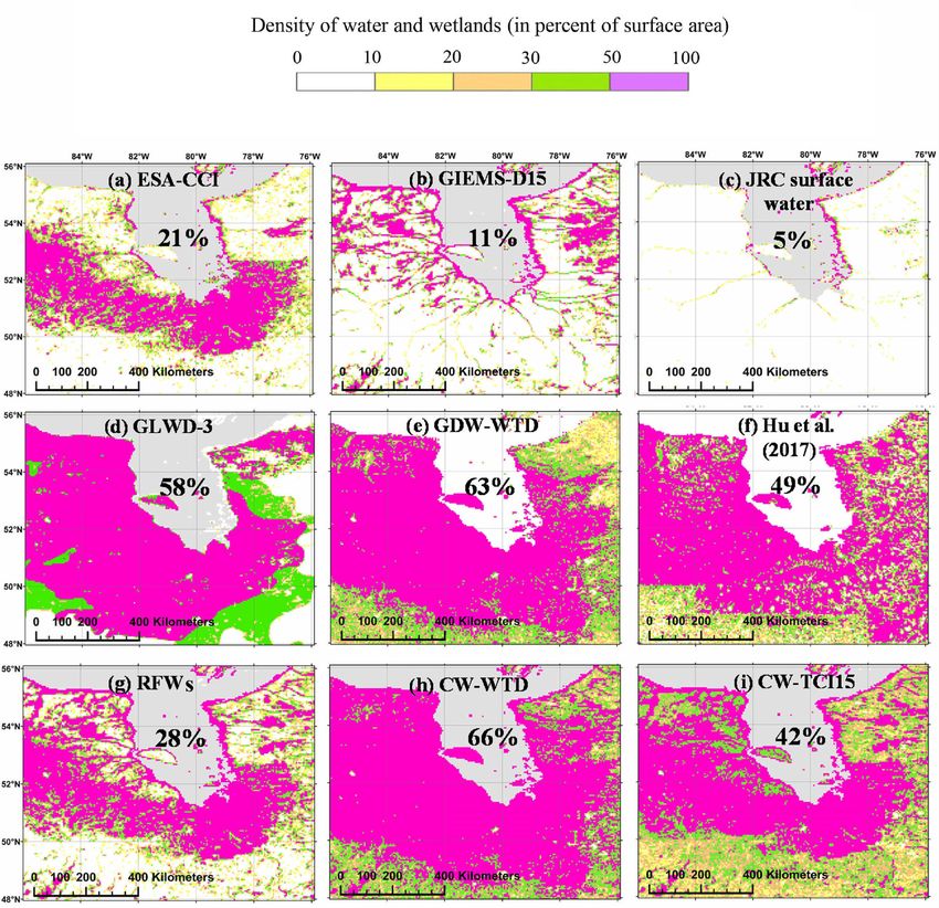
190                                         A. Tootchi et al.: Combining surface water imagery and groundwater constraints

1   Introduction                                                   mation. Fluet-Chouinard et al. (2015) developed the global
                                                                   inundation product GIEMS-D15 by downscaling the 0.25◦
Wetlands are valuable ecosystems with a key role in carbon,        multi-satellite wetland fractions of Prigent et al. (2007) us-
water and energy cycles (Matthews and Fung, 1987; Richey           ing 15 arcsec topography, with a global long-term maximum
et al., 2002; Repo et al., 2007; Ringeval et al., 2012). Wa-       inundation fraction of 13 %. Poulter et al. (2017) corrected
ter retention in wetlands leads to lower and delayed runoff        the wetland fractions of the surface water microwave product
peaks, higher base flows and evapotranspiration, which di-         series (SWAMPS; Schroeder et al., 2015) by merging them
rectly influence climate (Bierkens and van den Hurk, 2007;         with those obtained at 30 arcsec from GLWD.
Lin et al., 2016). Wetlands also serve to purify pollution            However, regardless of the wavelengths, wetlands derived
from natural and human sources, thus maintaining clean             from satellite imagery almost always represent inundated ar-
and sustainable water for ecosystems (Billen and Garnier,          eas and overlook other types of wetlands where soil mois-
1999; Dhote and Dixit, 2009; Curie et al., 2011; Passy et          ture is high but the surface is not inundated (Maxwell and
al., 2012). Despite their widely recognized importance, no         Kollet, 2008; Lo and Famiglietti, 2011; Wang et al., 2018).
consensus exists on wetland definitions and their respective       The method most frequently used to delineate these wet-
areal extents among the reviewed literature (Table 1). Based       lands is water table depth (WTD) modeling. Direct ground-
on several definitions, the extents range from regions with        water (GW) modeling (e.g., Miguez-Macho and Fan, 2012)
relatively shallow water tables (National Research Council,        requires in-depth knowledge of the physics of water move-
1995; Kutcher, 2008; Ramsar, 2009) to areas with permanent         ment, topography at a sufficiently high resolution, climate
inundation such as lakes (lacustrine wetlands) with depths of      variables, subsurface characteristics and observational con-
several meters. The reasons for this ambiguity are a diversity     straints (Fan et al., 2013; de Graaf et al., 2015). Simplified
of scientific points of views as well as the complexity of clas-   GW models based on the topographic index (TI) of TOP-
sification in transitional land features and temporally varying    MODEL (Beven and Kirkby, 1979) require less extensive
land features under human influences (Mialon et al., 2005;         input, and they have also been used to map wetlands (e.g.,
Papa et al., 2010; Ringeval et al., 2011; Sterling et al., 2013;   Gedney and Cox, 2003). Using the topography, the TI can be
Hu et al., 2017; Mizuochi et al., 2017).                           calculated as follows:
   The first global wetland maps were developed based on
                                                                                 a

a compilation of regional archives and estimates. Matthews         TI = ln             ,                                      (1)
                                                                              tan(β)
and Fung (1987) developed a 1◦ resolution wetland map
based on vegetation, soil properties and inundation fractions      where a(m) is the drainage area per unit contour length and
that covered ca. 4 % of the land. Finlayson et al. (1999)          tan(β) is the local slope at the desired pixel. The TI is often
based their estimates on surveys and the Ramsar global in-         presented as a wetness index (Wolock and McCabe, 1995;
ventory in which wetlands cover 9.7 % of the land area. Later,     Sørensen et al., 2006) because high values are found over flat
the Global Lakes and Wetlands Database (GLWD) was de-              regions, with large drainage areas corresponding to a high
veloped at 30 arcsec resolution (∼ 1 km at the Equator) by         propensity for saturation. Other environmental characteris-
compiling several national and regional wetland maps with          tics such as climate and soil or underground properties can
a global cover of 6.9 % of the land area, excluding Antarc-        also be used in the TI formulation to detect wetlands in ar-
tica and glaciated lands (Lehner and Döll, 2004). Because          eas where topography is not the primary driver of the water
satellite imagery permits homogeneous observation of land          budget, such as wetlands in uplands and over clayey soils or
characteristics, this method has been favored for mapping of       thin active layers in the permafrost region (e.g., Saulnier et
water-related features in recent decades. Satellite imagery at     al., 1997; Mérot et al., 2003; Hu et al., 2017).
visible wavelengths reports that 1.6 % to 2.3 % of Earth’s            A major challenge in the identification of wetlands through
land is permanently under water (Verpoorter et al., 2014;          GW modeling is the definition of thresholds on TI or WTD
Feng et al., 2015; Yamazaki et al., 2015; Pekel et al., 2016),     for separation of wetland from non-wetland areas. The
but with large disagreements (Nakaegawa, 2012), and inun-          thresholds are often calibrated to reproduce the extent of doc-
dations under densely vegetated and clouded areas are often        umented wetlands in a certain region and are subsequently
missed (Lang and McCarty, 2009). Longer wavelengths in             extrapolated for larger domains. This strategy was proven
the microwave band (e.g., L and C bands) penetrate better          successful at the basin scale (e.g., Curie et al., 2007), but it
through the cloud and vegetation layer and supply dynamic          has been shown to be ineffective at larger scales because it is
observations of inundated zones, usually with a trade-off be-      not possible to uniquely link TI values to soil saturation lev-
tween high resolution with a low revisit rate or domain extent     els across different landforms and climates (Marthews et al.,
(Li and Chen, 2005; Hess et al., 2015) and coarse resolution       2015). Hu et al. (2017) produced a global wetland map by
with a high revisit rate up to global coverage (Prigent et al.,    calibrating TI thresholds for every large basin of the world
2007; Papa et al., 2010; Schroeder et al., 2015; Parrens et al.,   based on land cover maps, as pioneered over France due to
2017). Recent progress has been achieved by downscaling or         independent TI threshold calibration in 22 hydro-ecoregions
correcting the latter products using higher-resolution infor-      using soil type datasets (Berthier et al., 2014). Uniform WTD

Earth Syst. Sci. Data, 11, 189–220, 2019                                            www.earth-syst-sci-data.net/11/189/2019/
A. Tootchi et al.: Combining surface water imagery and groundwater constraints                                                                                                           191

Table 1. Summary of water body, wetland and related proxy maps and datasets from the literature. The wet fractions indicated in % in the
last column are those indicated in the reference paper or data description for each study.

                                                                                                                                                          Wetland extent
   Name and reference                     Resolution                               Type of acquisition
                                                                                                                                               (million km2 )         % of the landa
   Maltby and Turner (1983)               –                                        Based on Russian geographical studies                                     8.6                 6.6 %
   Matthews and Fung (1987)               1◦                                       Development from soil, vegetation and                                    5.3b                 4.0 %
                                                                                   inundation maps
   Mitsch and Gosselink                   Polygons                                 Gross estimates, combination of estimates                             ∼ 20b              ∼ 15.3 %
   (2000)                                                                          and maps
   GLWD-3 (Lehner and                     30 arcsec, ∼ 1 km                        Compilation of national/international maps                        8.3–10.2c          6.2 %–7.6 %
   Döll, 2004)
   GLC2000 (Bartholomé and                1 km at Equator                          SPOT vegetation mission satellite observa-                                4.9                 3.4 %
   Belward, 2005)                                                                  tions
   GIEMS (Prigent et al.,                 0.25◦ , ∼ 25 km                          Multi-sensor: AVHRR, SSM/I, Scatterome-                              2.1–5.9            1.4 %–4 %
   2007)                                                                           ter ERS
   Fan et al. (2013)                      30 arcsec, ∼ 1 km                        Groundwater modeling                                                ∼ 19.3b                 ∼ 17 %
   GLOWABO (Verpoorter et                 Shapefiles of lakes larger               Satellite imagery: Landsat and SRTM                                          5                3.7 %
   al., 2014)                             than 0.002 km2                           topography
   SWAMPS (Schroeder et al.,              25 km                                    Modeling using multi-sensor info: SSM/I,                         7.7–12.5d           5.2 %–8.5 %
   2015)                                                                           SSM/S, QuikSCAT, ASCAT
   ESA-CCI land cover                     10 arcsec, ∼ 300 m                       Multi-sensor: SPOT vegetation, MERIS                                      6.1                 4.7 %
   (Herold et al., 2015)                                                           products
   GIEMS-D15                              15 arcsec, ∼ 460 m                       Multi-sensor: SSM/I, ERS-1, AVHRR,                                 6.5–17.3         5.0 %–13.2 %
   (Fluet-Chouinard et al.,                                                        downscaled from a 0.25◦ wetland map
   2015)
   G3WBM (Yamazaki et al.,                3 arcsec, ∼ 90 m                         Satellite imagery: Landsat                                                3.2                 2.5 %
   2015)
   Satellite imagery: Landsat,            2.8–4.4                                  2.1 %–3.4 %
   including maximum water
   extent and interannual
   occurrence
   HydroLAKES (Messager et                Shapefiles of lakes larger               Multiple inventory compilation including                                  2.7                 1.8 %
   al., 2016)                             than 0.1 km2                             Canadian hydrographic dataset and SWBD
   Hu et al. (2017)                       1 km                                     Development based on topographic wetness                               29.8e                22.5 %
                                                                                   index and land cover
   Poulter et al. (2017)                  0.5◦ , ∼ 50 km                           Merging SWAMPS and GLWD-3                                                10.5                 7.1 %
 a Percentages are those from the corresponding journal article or book. If no mention of percentage coverage exists, the value is calculated by dividing the wetland area by the land
 surface area excluding Antarctica, glaciated Greenland and lakes. b Excluding Caspian Sea and large lakes. c Excluding Antarctica, glaciated Greenland, lakes and Caspian Sea.
 Additionally the range in GLWD is different based on interpretation of fractional wetlands. d Excluding large water bodies. e Including the Caspian Sea.

thresholds (0 cm for inundated areas and 25 cm for wetlands)                                      eled WTD and TI, always implies subjective choices and can
are applied in the only example (to the best of our knowl-                                        result in over- or underestimation of wetland extents or unre-
edge) of direct global GW modeling for wetland delineation                                        alistic wetland distribution patterns.
(Fan and Miguez-Macho, 2011; Fan et al., 2013). All these                                            The scientific objective of the current work is to develop
datasets based on GW modeling estimate the wetland frac-                                          a comprehensive global wetland dataset based on a unique
tion as being much higher than those based on inventories                                         and applicable wetland definition for use in hydrological and
and satellite imagery (Hu et al., 2017: 22.6 %, Fan et al.,                                       land surface modeling. Based on the above analysis, our ra-
2013: 15 % of the land surface area). It must be emphasized                                       tionale is that inundated and groundwater-driven wetlands
that adjustment of wetland thresholds, both for directly mod-                                     must both be considered to realistically capture the wet-

www.earth-syst-sci-data.net/11/189/2019/                                                                                    Earth Syst. Sci. Data, 11, 189–220, 2019
192                                           A. Tootchi et al.: Combining surface water imagery and groundwater constraints

land patterns and extents. This approach leads to a definition         In this process, many layers were developed and are sum-
of wetlands as areas that are persistently saturated or near-       marized in Table 2 and detailed in Sect. 3. The map and
saturated because they are regularly subject to inundation or       methods to exclude lakes from all layers are explained in
shallow water tables. This definition is focused on hydro-          Sect. 2.2. Input datasets to RFWs and GDWs are presented
logical functioning, and is not restricted to areas with typ-       in Sect. 2.3 and 2.4, respectively, and several independent
ical wetland vegetation. In this context, although inundated        validation datasets, global and regional, are presented in
areas and zones with shallow groundwater partially overlap          Sect. 2.5. It should be noted that in the remainder of this pa-
and share similar environmental properties, they cannot be          per, the wetland percentages of the land surface area always
detected using a single method. Thus, we rely on data fu-           exclude lakes (Sect. 2.2), the Caspian Sea, the Greenland ice
sion methods, which have proven advantageous in develop-            sheet and Antarctica (unless otherwise mentioned). For this
ing high-quality products by merging properties from vari-          reason, these percentages and areas might be different from
ous datasets (Fritz and See, 2005; Jung et al., 2006; Schep-        those shown in Table 1, which are indicated for each original
aschenko et al., 2011; Pérez-Hoyos et al., 2012; Tuanmu and         paper or data description.
Jetz, 2014), including wetland mapping (Ozesmi and Bauer,
2002; Friedl et al., 2010; Poulter et al., 2017). In this frame-    2.2     Lakes
work, we tested several composite wetland (CW) maps, all
constructed at 15 arcsec resolution, by merging two comple-         To distinguish large permanent lakes and reservoirs from
mentary classes of wetlands: (1) regularly flooded wetlands         wetlands, we used the HydroLAKES database (Messager
(RFWs), where surface water can be detected at least once           et al., 2016), which was developed by compiling national,
a year through satellite imagery, and (2) groundwater-driven        regional and global datasets (Fig. 1a). This database con-
wetlands (GDWs) based on groundwater modeling.                      sists of more than 1.4 million individual polygons for lakes
   The main assumptions underlying the composite wetland            with a surface area of at least 10 ha, covering 1.8 % of the
maps are detailed in Sect. 2, together with the datasets in-        land surface area. It also classifies artificial dam reservoirs
volved. Subsequently, Sect. 3 sequentially presents the con-        which amount to 300 × 103 km2 (Messager et al., 2016). The
struction of the RFW, GDW and CW maps, with prelimi-                lakes’ extent in HydroLAKES is smaller than in other re-
nary analyses of their features and uncertainties. In Sect. 4,      cent databases that account for smaller water bodies: 2.5 %
we compare the CW maps with several validation wetland              in G3WBM (Yamazaki et al., 2015) for water bodies above
datasets, globally and in several areas with contrasting cli-       0.8 ha and 3.5 % in GLOWABO (Verpoorter et al., 2014)
mates and wetland fractions, to show that the combination of        for those above 0.2 ha. These two datasets do not differ-
RFWs and GDWs provides a consistent wetland description             entiate lakes from other surface water elements, and using
throughout the globe. This comparison allows us to select           them as a mask would lead to the exclusion of shallow in-
two CW maps with better overall performances, used to dis-          undated portions of wetlands (e.g., Indonesian mangroves or
cuss the role of GDWs in Sect. 5. Finally, the availability and     Ganges floodplains). It must also be noted that the small wa-
potential applications of the composite maps are presented in       ter bodies tend to be overlooked after dominant resampling
Sect. 6, while Sect. 7 summarizes the advantages and limita-        to 15 arcsec resolution (Sect. 2.6), unless they are sufficiently
tions of the approach and gives perspectives on future devel-       numerous in a pixel. Therefore, the lake mask covers 1.7 %
opments.                                                            of the land area compared with 1.8 % in the original Hydro-
                                                                    LAKES database. This map also shows that most of the lakes
                                                                    are located in the northern boreal zones (more than 60 % of
2     Datasets
                                                                    lakes area are located north of 50◦ N), in agreement with the
                                                                    other lake databases.
2.1    Mapping strategy and requirements
Based on the inclusive assumptions for wetland mapping in           2.3     Input to RFW map: inundation datasets
this study, we use GIS tools to construct several composite
wetland maps as the overlap (union) of the following:               2.3.1    ESA-CCI land cover

    – one RFW map developed by overlapping three sur-               This dataset succeeds the GlobCover dataset based on the
      face water and inundation datasets derived from satel-        data from the MERIS sensor (onboard ENVISAT) collected
      lite imagery in an attempt to fill the observation gaps       at high resolution for surface water detection, together with
      (Sect. 3.1);                                                  the SPOT-VEGETATION time series (Herold et al., 2015) to
                                                                    aid in distinguishing wetlands from other vegetation covers.
    – one GDW map out of seven, all derived from GW mod-            Global land cover maps at approximately 300 m (10 arcsec)
      eling (either direct or simplified based on several TI ver-   resolution deliver data for three 5-year periods (1998–2002,
      sions) and meant to sample the uncertainty of the GDW         2003–2007 and 2008–2012). The extents of water bodies
      contribution (Sect. 3.2).                                     slightly changed between the first 5-year period and the third
                                                                    one (such as shrinking of the Aral Sea area by more than

Earth Syst. Sci. Data, 11, 189–220, 2019                                             www.earth-syst-sci-data.net/11/189/2019/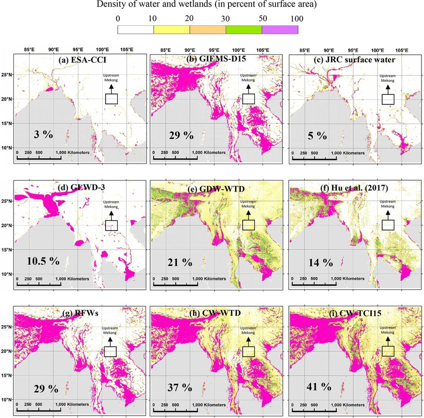
A. Tootchi et al.: Combining surface water imagery and groundwater constraints                                                            193

Table 2. Layers of wetlands constructed in the paper, their definitions and the subsections in which they are explained. The total land area
for wetland percentages excludes lakes, Antarctica and the Greenland ice sheet.

                                                                                                                 Wetland    Explained
        Layer                                     Definition
                                                                                                               percentage   in
        RFWs (regularly flooded wetlands)         Union of three inundation datasets (ESA-CCI, GIEMS-              9.7 %    Sect. 3.1
                                                  D15, JRC surface water)
                                 WTD              Pixels with water table depth less than 20 cm (Fan et al.,        15 %    Sect. 3.2.1
                                                  2013)
                                 TI          6    Pixels with highest TIs, covering 15 % of total land               6%
                                                  when combined with RFWs
        GDWs                                15    Pixels with highest TIs values covering 15 % of land              15 %
        (groundwater-driven      TCI        6.6   Pixels with highest TCIs, covering 15 % of total land            6.6 %    Sect. 3.2.2
        wetlands)                                 when combined with RFWs
                                            15    Pixels with highest TCI values covering 15 % of land              15 %
                                 TCTrI       6    Pixels with highest TCTrI, covering 15 % of total land             6%
                                                  when combined with RFWs
                                            15    Pixels with highest TCTrI values covering 15 % of land            15 %
                                 WTD              Union of RFW and GDW-WTD                                        21.1 %
                                 TI          6    Union of RFW and GDW-TI6                                         15 %
        CW                                  15    Union of RFW and GDW-TI15                                       22.2 %
        (composite wetland)      TCI        6.6   Union of RFW and GDW-TCI6.6                                       15 %    Sect. 3.3
                                            15    Union of RFW and GDW-TCI15                                      21.6 %
                                 TCTrI       6    Union of RFW and GDW-TCTrI6                                      15 %
                                            15    Union of RFW and GDW-TCTrI15                                    22.3 %

55 %), but the extent of wetland classes (permanent wetlands             respectively). In this study, we assumed that the mean an-
and flooded vegetation classes) did not change significantly             nual maximum extent was the best representative measure
(the variation in wetland classes throughout these periods is            for wetlands. In the following, GIEMS-D15 always indicates
less than 3 % of the total wetlands area). We acquired the last          the mean annual maximum of GIEMS-D15 (Fig. 1c). Higher-
epoch data to represent the current state of wetlands (Fig. 1b).         resolution (3 arcsec) downscaling of GIEMS has been re-
In ESA-CCI, wetlands are mixed classes of flooded areas                  cently developed (Aires et al., 2017), but we overlooked this
with tree covers, shrubs or herbaceous covers plus inland wa-            source because we focused our study on 15 arcsec resolution.
ter bodies, covering 3 % of the Earth land surface overall.
                                                                         2.3.3    JRC surface water (Pekel et al., 2016)
2.3.2    GIEMS-D15 (Fluet-Chouinard et al., 2015)                        The JRC surface water products are a set of high-resolution
                                                                         maps (1 arcsec, ∼ 30 m) for permanent water and also for
Prigent et al. (2007) used multi-sensor satellite data, includ-
                                                                         seasonal and ephemeral water bodies. These products are
ing passive and active microwave measurements, together
                                                                         based on analysis of Landsat satellite images (Wulder et al.,
with visible and near-infrared reflectance to map the monthly
                                                                         2016) over a period of 32 years (1984–2015). Each pixel was
mean inundated fractions at 0.25◦ resolution for a 12-year pe-
                                                                         classified as open water, land or a nonvalid observation. Open
riod (1993–2004). This dataset (GIEMS) gives the minimum
                                                                         water is defined as any pixel with standing water, including
and maximum extent of the inundated area (including wet-
                                                                         fresh and saltwater. The study also quantifies the conversions,
lands, rivers, small lakes and irrigated rice). Fluet-Chouinard
                                                                         mostly referring to changes in state (lost or gained water ex-
et al. (2015) used the GLC2000 land cover map (Bartholomé
                                                                         tents, conversions from seasonal to permanent, etc.) during
and Belward, 2005) to train a downscaling model for GIEMS
                                                                         the observation period. In this study, we used the maximum
at 15 arcsec resolution based on the HydroSHEDS digital
                                                                         surface water extent, which consists of all pixels that were
elevation model (Lehner et al., 2008) and developed three
                                                                         under water at least once during the entire period, covering
static datasets for mean annual minimum, mean annual max-
                                                                         almost 1.5 % of the Earth land surface area (Fig. 1d).
imum and long-term maximum extent of the inundated areas
(covering 3.9 %, 7.7 % and 10.3 % of the land surface area,

www.earth-syst-sci-data.net/11/189/2019/                                                      Earth Syst. Sci. Data, 11, 189–220, 2019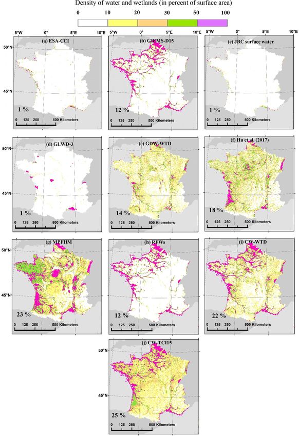
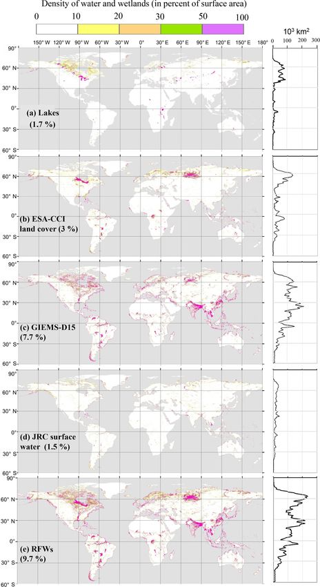
194                                             A. Tootchi et al.: Combining surface water imagery and groundwater constraints

Figure 1. Density of lakes, regularly flooded wetlands and components of the latter (percent area in 3 arcmin grid cells). For zonal wetland
area distributions (right-hand charts), the area covered by wetlands in each 1◦ latitude band is displayed.

Earth Syst. Sci. Data, 11, 189–220, 2019                                                     www.earth-syst-sci-data.net/11/189/2019/
A. Tootchi et al.: Combining surface water imagery and groundwater constraints                                               195

2.4     Input to GDW maps                                         land delineation by including other environmental factors or
                                                                  modifying the formulation of the wetness index (Rodhe and
2.4.1    Water table depth estimates (Fan et al., 2013)
                                                                  Seibert, 1999; Mérot et al., 2003; Manfreda et al., 2011).
Fan et al. (2013) performed global GW modeling to esti-           Therefore, we used the global TI dataset of Marthews et
mate the water table depth at 1 km resolution. This model         al. (2015) to supply the original TI, and also as a base map to
assumes a steady flow, and lateral water fluxes are calculated    derive two other variants of the index.
using Darcy’s law and the Dupuit–Forchheimer approxima-              The first variant index is the TCI (topography–climate
tion for 2-D flow. Elevation is described at 30 arcsec reso-      wetness index, inspired by Mérot et al., 2003):
lution (by HydroSHEDS south of 60◦ N and otherwise by
                                                                               a · Pe

ASTER/NASA-JPL), and the recharge rates were modeled at           TCI = ln              = TI + ln(Pe ),                       (2)
                                                                              tan(β)
0.5◦ resolution using the WaterGAP model (Döll and Fiedler,
2008) based on contemporary meteorological forcing (1979–         where Pe is the mean annual effective precipitation (in
2007). To estimate subsurface transmissivity, the soil hy-        meters). The effective precipitation is first defined at the
draulic conductivities were derived from the global Food and      monthly time step as the monthly precipitation Pm,y (in me-
Agriculture Organization (FAO) digital soil maps (5 arcmin        ters) for month m and year y that is not evaporated or tran-
resolution) and US Department of Agriculture (USDA) soil          spired using the monthly potential evapotranspiration EPm,y
maps over the United States (30 arcsec resolution) and sub-       (in meters) as a proxy for total evapotranspiration:
sequently assumed to decay exponentially with depth from           e
                                                                  Pm,y = max(0, Pm,y − EPm,y ).                               (3)
the thin soil layer (2 m) down as a function of the local to-
                                                                  Pe is subsequently calculated as the sum of the 12 pluri-
pographic slope. The decay factor is also adjusted for the
                                                                  annual means of monthly effective precipitation. The re-
permafrost region using an additional thermic factor (smaller
                                                                  quired climatic variables are taken from the CRU monthly
transmissivity in permafrost areas). The modeled WTD was
                                                                  meteorological datasets (Sect. 2.2.3) for 1980–2016 to repre-
compared to observations available to the authors (more than
                                                                  sent the contemporary period.
1 million observations, with 80 % of them located in North
                                                                     The second variant index (known as TCTrI, topography–
America). The resulting dataset suggests vast areas with a
                                                                  climate–transmissivity index) is constructed by combining
shallow water table over the tropics, along the coastal zones
                                                                  the effect of heterogeneous transmissivity (Rodhe and Seib-
and in boreal areas of North America and Asia (almost 15 %
                                                                  ert, 1999) with the above TCI:
of the land area for WTD ≤ 20 cm).
                                                                                   a · Pe
                                                                  TCTrI = ln                   = TI + ln(Pe ) − ln(Tr),     (4)
2.4.2    Three maps of topographic wetness indices                               Tr · tan(β)
                                                                  where Tr (m2 s−1 ) is the transmissivity calculated by verti-
Flat downstream areas display a marked propensity to be sat-
                                                                  cally integrating a constant Ks (saturated hydraulic conduc-
urated, which explains the wide use of topographic indices to
                                                                  tivity in m s−1 ) from GLHYMPS over the first 100 m below
delineate wetlands. Here, we use the global map of TI pro-
                                                                  the Earth’s surface (Sect. 2.4.4).
duced by Marthews et al. (2015) at 15 arcsec resolution. It re-
lies on the original formulation of Beven and Kirkby (1979),
as in Eq. (1), and on two global high-resolution digital el-      2.4.3   CRU climate variables
evation models (DEMs), viz. HydroSHEDS (Lehner et al.,            To assess the impact of climate on wetlands, we used
2008) and Hydro1k (US Geological Survey, 2000) at 15 and          the Climatic Research Unit (CRU) monthly meteorological
30 arcsec resolution, respectively. Hydro1k is used to fill the   datasets. These datasets cover all land area from the be-
lack of information in HydroSHEDS north of 60◦ N, which           ginning of the twentieth century (Harris et al., 2014). CRU
is outside of the SRTM (Shuttle Radar Topography Mis-             climate time series are gridded to 0.5◦ resolution based on
sion) coverage. Because index values depend on pixel size,        more than 4000 individual weather station records. To in-
which varies with latitude, those researchers also applied        clude a climate factor in the TI formulations, the time series
the dimensionless topographic wetness index correction of         of selected climate variables (i.e., precipitation and potential
Ducharne (2009) to transform the index values to equivalents      evapotranspiration based on the Penman–Monteith equation)
for a 1 m resolution.                                             are extracted for the contemporary period (1980–2016).
   Topography, however, is often not sufficient for wetland
identification because climate and subsurface characteristics
                                                                  2.4.4   GLHYMPS (Gleeson et al., 2014)
also control water availability and vertical drainage. Using
the original TI formulation in Eq. (1), high index zones might    GLHYMPS is a global permeability and porosity map
coincide with flat arid areas, or inversely, low index values     based on high-resolution lithology (Hartmann and Moos-
might occur at wetland zones with small upstream drainage         dorf, 2012). The permeability dataset and its derived hy-
areas over a shallow impervious layer. Several studies have       draulic conductivity (Ks ) estimates are given in vector for-
focused on improving the topographic wetness index for wet-       mat, with an average polygon size of approximately 100 km2 .

www.earth-syst-sci-data.net/11/189/2019/                                            Earth Syst. Sci. Data, 11, 189–220, 2019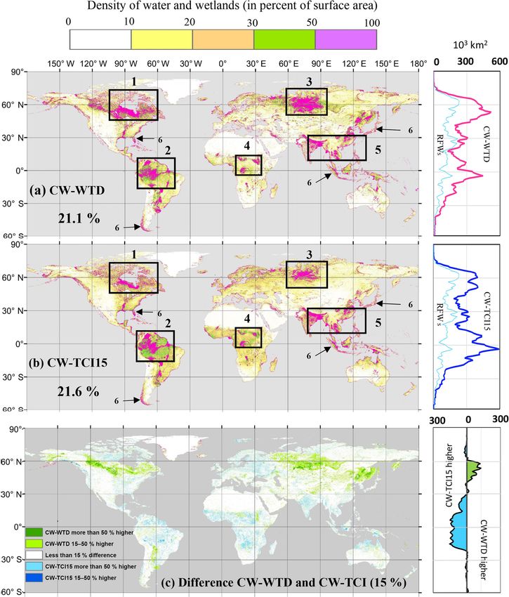
196                                          A. Tootchi et al.: Combining surface water imagery and groundwater constraints

As noted by the developers of GLHYMPS (Gleeson et al.,              2.5.2   Global wetland potential distribution (Hu et al.,
2011, 2014), “lithology maps represent the shallow subsur-                  2017)
face (on the order of 100 m)”, and thus hydraulic conduc-
                                                                    Hu et al. (2017) proposed a potential wetland distribution us-
tivity estimates are valid for the first 100 m of the subsur-
                                                                    ing a precipitation topographic wetness index based on a new
face layer. Thus, we estimated transmissivity as the integral
                                                                    TI formulation in which the drainage area is multiplied by
of this constant Ks over these 100 m and used it to check
                                                                    the mean annual precipitation. This formulation is based on
whether use of the available transmissivity datasets in TI
                                                                    the concept of the topography–climate wetness index (Mérot
formulations can improve global wetland identification. It
                                                                    et al., 2003) in which the effective precipitation was intro-
should be noted that the hydraulic conductivity dataset has
                                                                    duced as the climate factor. The new index is calculated at
two versions: with and without the permafrost effect. To con-
                                                                    1 km resolution using GTOPO30 elevation data developed by
sider the permafrost effect, Gleeson et al. (2014) used maps
                                                                    the USGS. Wetlands are categorized into “water” and “non-
of the permafrost zonation index (PZI) from Gruber (2012)
                                                                    water” wetlands based on regionally calibrated thresholds for
and homogenously assigned a rather low hydraulic conduc-
                                                                    each large basin of the world (level-1 drainage area of Hy-
tivity (Ks = 10−13 m s−1 ) for areas with PZI > 0.99, i.e.,
                                                                    dro1k) using a sample trained adjustment model. The water
in Siberian taiga forests and tundra, the Canadian Arctic
                                                                    classes of several land cover datasets are used to train the
Archipelago and Greenland. This choice leads to a very large
                                                                    model for the water threshold, and the model for the non-
contrast of Ks and transmissivity between permafrost and
                                                                    water wetland threshold is trained on the regularly flooded
non-permafrost zones, which largely overrules the effects of
                                                                    tree cover and herbaceous cover categories (additional details
lithology, so the high TI values (potential wetlands) become
                                                                    are available in the Supplement, Sect. S1 and Fig. S2). The
concentrated in permafrost areas. To preserve the influence
                                                                    global coverage of the water and non-water wetland classes
of lithology, we rasterized the vector polygons of Ks without
                                                                    in Hu et al. (2017) is 22.6 % of the Earth land surface area
the permafrost effect to 15 arcsec resolution.
                                                                    (excluding lakes, Antarctica and the Greenland ice sheet),
                                                                    considering no loss due to human influence. This dataset
2.5     Validation datasets                                         gives the largest wetland extent within the accessible liter-
Two global and two regional wetland datasets were used to           ature, with notably large water wetlands in South America
assess the validity of the CW maps, and none of them were           and large non-water wetlands in central Asia and the North
used as inputs to the composite wetland maps to ensure an           American continent. In this paper, we used the union of the
independent evaluation of the strengths and weaknesses of           water and non-water wetland classes of this dataset for fur-
the CW maps.                                                        ther evaluations.

2.5.1    GLWD-3 (Lehner and Döll, 2004)                             2.5.3   Amazon basin wetland map (Hess et al., 2015)

The GLWD, the Global Lakes And Wetlands Dataset, is                 Hess et al. (2015) used the L-band synthetic aperture radar
based on the aggregation of regional and global land cover          (SAR) data from the Japanese Earth resources satellite
and wetland maps. This dataset contains three levels of in-         (JRES-1) imagery scenes at a 100 m resolution to map wet-
formation, and the most inclusive one is GLWD-3, which is           lands during the period 1995–1996 for high and low water
in raster format. This dataset has an original 30 arcsec resolu-    seasons. The studied domain excludes zones with altitudes
tion and contains 12 classes for lakes and wetlands (maps and       higher than 500 m and corresponds to a large fraction of
details are given in the Supplement, Sect. S1 and Fig. S1).         the Amazon basin (87 %). Wetlands are defined as the sum
For large zones prone to water accumulation but without             of lakes and rivers (both covering 1 % of the basin area)
solid information on existing wetlands, fractional wetland          and other flooded areas plus zones not flooded but adjacent
classes are defined (together they cover 4 % of the land sur-       to flooded areas and sharing wetland geomorphology. The
face area). This is particularly the case within the Prairie Pot-   flooded fraction of wetlands varies considerably (from 38 %
hole Region in North America and the Tibetan Plateau in             to 75 %) between the low and high water season. The total
Asia. Depending on the interpretation of fractional wetlands        maximum mapped wetland area extends over 0.8 million km2
(by taking either the minimum, mean or maximum fraction             and is used in the evaluation of CW maps in this study.
of the ranges), wetlands cover between 5.8 % and 7.2 % of
the land surface area. In this paper, we take the mean fraction     2.5.4   Modeled potentially wet zones of France
in these areas, leading to a total wetland extent of 6.3 % of
                                                                    The map of potentially wet zones in France (les Milieux
the land surface area.
                                                                    Potentiellement Humides de France Modélisée, MPHFM;
                                                                    Berthier et al., 2014) constructed at a 50 m resolution is based
                                                                    on the topo-climatic wetness index (Mérot et al., 2003) and
                                                                    the elevation difference to streams using the national high-
                                                                    resolution DEMs. Meteorological data for the calculation of

Earth Syst. Sci. Data, 11, 189–220, 2019                                             www.earth-syst-sci-data.net/11/189/2019/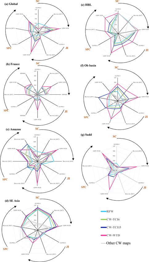
A. Tootchi et al.: Combining surface water imagery and groundwater constraints                                                 197

the topo-climatic index (precipitation and potential evapora-           Based on this definition, another feature of the proposed
tion rates; see further details in Sect. 3.2.2) are taken from the   wetland maps is that they are static. As stated in Prigent
SAFRAN atmospheric reanalysis (Vidal et al., 2010) at 8 km           et al. (2007), the maps represent the “climatological max-
resolution. Index thresholding for wetland delineation is per-       imum extent of active wetlands and inundation” (for CWs
formed independently in 22 hydro-ecoregion units and de-             and RFWs, respectively), i.e., the areas that happen to be
limited based on lithology, drainage density, elevation, slope,      saturated or near-saturated sufficiently frequently to develop
precipitation rate and temperature. The wet fraction defin-          specific features of wetlands (high soil moisture over a sig-
ing the threshold in each hydro-ecoregion is the fraction            nificant period of the year, potentially leading to reducing
of hydromorphic soils (extrapolated from local soil maps             conditions in selected horizons and specific flora and fauna).
to almost 18 % of the area of metropolitan France) taken
from national soil maps at 1 : 250 000 (InfoSol, 2013). Ad-
                                                                     3.1.2    Data processing
ditionally, the elevation difference between land pixels and
natural streams was used to separate large streambeds and            To project, resample, intersect/overlap and convert different
plain zones, which are difficult to model with indices based         datasets used in wetland mapping in this study, we relied
on topography. Based on MPHFM, potential wetlands ex-                on ArcMap software (Esri, ArcGIS Desktop: Release 10.3.1
tend over almost 130 000 km2 of France (23 % of the area             Redlands, CA) and its different tools. All datasets were pro-
of metropolitan France). The dataset was validated against           jected to a WGS84 equi-rectangular coordination system and
available pedological point data (based on profiles or sur-          subsequently resampled to a single resolution for facilitated
veys) available over France. These point data are classified         fusion and comparison. The resulting raster datasets were
into wetlands and non-wetlands for the validation procedure.         processed with ArcMap tools available in almost any GIS
This procedure used statistical criteria such as spatial coinci-     software such as QGIS (Table 3).
dence (SC; number of correctly diagnosed points over total               The final resolution of the maps is targeted to 15 arcsec
number of points) and the kappa coefficient (modeling error          (∼ 500 m at the Equator) for consistency with the avail-
compared with a random classification error).                        able water datasets. Therefore, all datasets were resampled
                                                                     to 15 arcsec resolution, which is within the resolution range
3     Construction of composite wetland maps                         of state-of-the-art wetland-related datasets. For datasets at
                                                                     coarser resolutions, each coarse pixel is disaggregated to
3.1     Definitions and layer preparation                            15 arcsec while retaining the same value. We used an “all-or-
                                                                     nothing” approach; i.e., the pixels are either fully recognized
3.1.1    Wetland definition
                                                                     as wetland (or lake) or not at all, based on the dominant type
The wetland definition behind the composite maps is focused          if the input data are finer than 15 arcsec (ESA-CCI land cover
on hydrological functioning, and we aim to include both sea-         and JRC surface water).
sonal and permanent wetlands as well as shallow surface wa-              Eventually, each 15 arcsec global raster contains more than
ter bodies (including rivers, both permanent and intermit-           80 000 pixels along a circle of 360◦ of longitude, and wet-
tent). Surface water bodies and wetlands are often hydro-            lands can exhibit notably small-scale patterns (e.g., patchy
logically connected, and the transition between them is not          or river-like). To facilitate visual inspection, we calculated
sharp and varies seasonally. Moreover, these features are dif-       the mean wetland densities in 3 arcmin grids for most of the
ficult to separate based on observations (either in situ or re-      maps presented in this work. The same 3 arcmin resolution
mote), and no dedicated exhaustive dataset is currently avail-       (∼ 6 km at the Equator) was used in calculating the spatial
able (Raymond et al., 2013; Schneider et al., 2017). Inclu-          correlations. For zonal wetland area distributions, the area
sion of the shallow surface water bodies (in the RFW map)            covered by wetlands in each 1◦ latitude band is displayed.
is compatible with the Ramsar classification, but we depart
from this approach with respect to large permanent lakes,
                                                                     3.2     Regularly flooded wetland (RFW) maps
which are excluded from all input datasets to RFW and GDW
maps (Sect. 2.2) because of their distinct hydrology and             3.2.1    Mapping by data fusion
ecology compared with wetlands. In contrast, groundwater-
driven wetlands can remain wet without inundation due to             To identify the RFWs, we overlapped carefully selected
the presence of shallow water tables. As further discussed in        datasets of surface water, land cover and wetlands, namely,
Sect. 3.2, these areas are defined in this study as areas where      the ESA-CCI land cover, GIEMS-D15 inundation surface
the mean annual WTD is less than 20 cm, following similar            and the maximum water extent in JRC surface water. These
assumptions in the literature (US Army Corps of Engineers,           datasets were selected to include different types of data ac-
1987; Constance et al., 2007; Tamea et al., 2010; Fan and            quisition. The idea behind the fusion approach chosen in
Miguez-Macho, 2011).                                                 this work is that wetlands identified by the different datasets
                                                                     are all valid despite their uncertainties, although none of
                                                                     them are exhaustive. As a result, use of multiple inundation

www.earth-syst-sci-data.net/11/189/2019/                                               Earth Syst. Sci. Data, 11, 189–220, 2019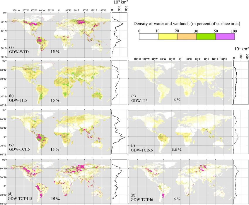
198 A. Tootchi et al.: Combining surface water imagery and groundwater constraints
Table 3. ArcMap tools used in this study for data processing and their equivalent open-source software.
ArcMap Open-source software Application
Polygon to raster (Conversion toolbox) Rasterize (vector to raster) To convert vector data into raster pixels
Project raster (Data Management toolbox) QGIS: Warp (reproject) Projecting different layers coordinate
system to WGS84
Resample & Aggregate (Data Management toolbox) QGIS: Raster Calculator To change the resolution of the rasters
Raster Calculator (Spatial Analyst toolbox) QGIS: Raster Calculator To intersect/overlap raster datasets
Reclassify (Spatial Analyst toolbox) QGIS/GRASS: r.reclass To merge raster datasets or mask them
datasets fills the observational gap. Several other surface wa- shield are the main hotspots of peat in the American con-
ter datasets exist that were not used in this work, either be- tinent. The same situation exists in the West Siberian Plain
cause they mostly consist of lakes or because they rely on as well. The second zonal peak in RFWs lies between 20
similar methodologies (Verpoorter et al., 2014; Yamazaki et and 33◦ N, where the major contributors are the vast flood-
al., 2015). plains surrounding the Mississippi, Brahmaputra, Ganges,
Yangtze and Yellow rivers and Mesopotamian Marshes. A
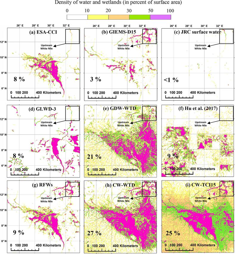
3.2.2 Geographic analysis total of 30 % of the world’s RFWs are found in tropical re-
gions (20◦ N to 20◦ S), concentrated mainly in the Amazon,
Overall, the RFW map covers 9.7 % of the land surface area Orinoco and Congo river floodplains and in inundated por-
(12.9 million km2 ) including river channels, deltas, coastal tions of wetlands such as the Sudd swamp in South Sudan.
wetlands and flooded lake margins (Fig. 1e). Areal coverage
of the RFWs is by definition larger than the area of wetlands
in all three input datasets (Fig. 1b–d), which were selected to 3.3 Groundwater-driven wetland (GDW) maps
be representative of different types of data acquisition (sen- 3.3.1 Mapping based on WTD
sors and wavelengths). Therefore, they correspond to differ-
ent definitions of inundated areas, and their contribution to Due to a lack of integrated, standardized and globally dis-
the RFW map is fairly different. In particular, the shared frac- tributed WTD observations, a sound approach to the loca-
tion of the three input maps is minuscule (5 % of the total tion of groundwater-driven wetlands is the use of available
RFW land surface area coverage), and is mostly composed global direct GW modeling results. In this study, we used the
of the large river corridors and ponds which are detectable by global WTD estimations of Fan et al. (2013), and the result-
satellite visible range imaging techniques in the JRC dataset. ing wetland map is denoted as GDW-WTD. As explained in
The latter misses most understory inundations, which are bet- Sect. 3.1.1 we assumed the mean annual WTD in wetlands
ter identified by the ESA-CCI dataset owing to specific veg- to be less than 20 cm, which results in a wetland area extend-
etation classification. Finally, owing to the use of microwave ing over 15 % of the land surface, with large wetlands in the
sensors, GIEMS-D15 extends over larger areas since it cap- northern areas and the Amazon basin (Fig. 2a). We also per-
tures both flooded areas and wet soils below most vegeta- formed a sensitivity analysis on the areal fraction of wetlands
tion canopies except the densest ones (Prigent et al., 2007). with different WTD thresholds (Sect. S2, Figs. S3 and S4),
In addition, the distribution of wetlands in GIEMS-D15 in- revealing that the variation in total wetland fraction is quite
volves downscaling as a function of topography, and can be weak (between 13.7 % and 16.7 %) for thresholds ranging
very different from the other datasets. Hence, 58 % of RFWs from 0 to 40 cm. Therefore, a 20 cm threshold appears to be a
are solely sourced from GIEMS-D15, mostly in the South- credible representative value. However, the wetland fraction
east Asian floodplains, Northeast Indian wet plains and rice rapidly increases for deeper thresholds, showing that a clear
paddies, and the Prairie Pothole Region (in the northern US distinction exists between shallow WTD areas (wetlands ac-
and Canada). The ESA-CCI contribution is mainly found in cording to our definition) and the remainder of the land.
the Ob River basin where wetland vegetation exists but wet
soils are not easily detected by visible (JRC) or microwave 3.3.2 Mapping based on various TIs
(GIEMS-D15) observation. Due to its high resolution, JRC
surface water adds small-scale wetlands such as patchy wet- In line with many studies (Rodhe and Seibert, 1999; Curie
lands, small ponds and oases (0.4 % of the land surface area). et al., 2007; Hu et al., 2017), we define TI-based wetlands
In terms of zonal distribution, 31 % of the RFWs are con- as the pixels with a TI above a certain threshold, defined to
centrated north of 50◦ N, with most of the wetlands formed match a certain fraction of total land. In doing so, we pre-
in the Prairie Pothole Region and Siberian lowlands. Cold scribe the global GDW fraction as a chosen value, and the
and humid climates and the poorly drained soils of the bo- various TI formulations (Sect. 2.4.2) only change the geo-
real forest regions in northern Canada on the Precambrian graphic distribution of the corresponding wetlands. To ap-
Earth Syst. Sci. Data, 11, 189–220, 2019 www.earth-syst-sci-data.net/11/189/2019/A. Tootchi et al.: Combining surface water imagery and groundwater constraints 199
Figure 2. Density of scattered groundwater wetlands based on different approaches (percent area in 3 arcmin grid cells). For zonal wetland
area distributions (right-hand charts), the area covered by wetlands in each 1◦ latitude band is displayed.
prehend the uncertainty related to the choice of the global and GDW-TCTrI15, with diminished extents and densities
GDW fraction, we tested two choices within the bounds de- (Fig. 2e–g).
rived from the global WTDs of Fan et al. (2013). In the first
approach, we set the TI threshold such that the wet pixels 3.3.3 Comparison of the proposed GDW maps
(with high index values) cover 15 % of the land surface area,
such as the fraction of WTD ≤ 20 cm according to Fan et As shown in Table 2, seven GDW maps are developed,
al. (2013). The corresponding maps are noted as GDW-TI15, consisting of GDW-WTD (Sect. 3.2.1) and six GDW-TIs
GDW-TCI15 and GDW-TCTrI15 in Table 2 and show fairly (Sect. 3.2.2). The GDW-WTD map contains high wetland
different patterns (Fig. 2b–d). The second approach assumes extents over the northern latitudes (Fig. 2a), in contrast to
that the total wetland extent (this time including both GDWs the other six GDW maps. The diagnosed wetlands of GDW-
and RFWs) covers 15 %. The TI thresholds are subsequently TI maps (Fig. 2b, e) are equally distributed over well-known
set such that the union of RFWs and GDW-TI (TCI/TCTrI), arid areas such as the Sahara and the Kalahari Desert, the
i.e., the composite wetlands, has the same extent as GDW- Australian Shield and the Arabian Peninsula as in wet re-
WTD. The resulting GDWs cover between 6 % and 6.6 % of gions such as the West Siberian Plain and northern Canada
the land area depending on the TI formulation and level of (Fig. 2b, e). As a result, for a given threshold (15 % in
overlap with RFWs (Table 4) and are noted as GDW-TI6, Fig. 3a), the distribution of wetlands derived from the simple
GDW-TCI6.6 and GDW-TCTrI6. The patterns of these three TI is nearly uniform over different latitudes. Lower thresh-
maps are highly similar to those of GDW-TI15, GDW-TCI15 olds on TI variants (Figs. 2e–g and 3b) obviously result in
a smaller wetland extent, with no major change in the zonal
www.earth-syst-sci-data.net/11/189/2019/ Earth Syst. Sci. Data, 11, 189–220, 2019200 A. Tootchi et al.: Combining surface water imagery and groundwater constraints Figure 3. Latitudinal distribution of different wetland maps: (a, b) GDWs, (c) components of CW-TCI15 and their intersection and (d, e) CWs. The wetland areas along the y axis are surface areas in each 1◦ latitudinal band. Earth Syst. Sci. Data, 11, 189–220, 2019 www.earth-syst-sci-data.net/11/189/2019/
A. Tootchi et al.: Combining surface water imagery and groundwater constraints                                               201

Table 4. Percent of overlap between GDWs and RFWs (percent of     (Table 4). These intersection zones are further discussed in
total land pixels).                                               Sect. 4. The wetland extent in CWs is by definition larger
                                                                  than both RFWs and GDWs, and their spatial patterns de-
      Groundwater-driven   Intersecting   Non-intersecting        pend on the contribution percentage of each component. As
      wetland layer        with RFWs          with RFWs           an example, in CW-TCI15, over most latitudes, the spatial
      GDW-TI6                    0.7 %              5.3 %         pattern is similar to that of RFWs, except over the tropical
      GDW-TCI6.6                 1.3 %              5.3 %         zones where GDWs are far more extensive than RFWs, thus
      GDW-TCTrI6                 0.7 %              5.3 %         shaping the general latitudinal pattern (Fig. 3c). Changing the
      GDW-TI15                   2.5 %             12.5 %         percentage of GDWs (between 6 % and 15 %) based on dif-
      GDW-TCI15                  3.6 %             11.4 %         ferent TI formulations increases the wetland fraction of the
      GDW-TCTrI15                2.4 %             12.6 %         CW maps to between 5.3 % and 12.5 % of the land area, but it
      GDW-WTD15                  3.8 %             11.2 %         does not considerably change their overall latitudinal pattern
                                                                  (Fig. 3d, e). In RFWs, large wetlands are present between 25
                                                                  and 35◦ N (Fig. 3c), whereas in all GDW maps, the wetland
pattern when the wet fraction threshold changes from 15 %         extents over these latitudes are smaller than in other wetland
to 6 % (Figs. 2b–d and 3a, b).                                    regions (Fig. 3a, b).
   Introducing a climate factor in the form of effective pre-
cipitation in GDW-TCI6.6 and GDW-TCI15 increases the              4     Validation
value of the wetness index in wet areas and decreases it in
dry climates (Figs. 2c, f and 3a, b). Therefore, previously di-   4.1    Spatial similarity assessment
agnosed wetlands with a TI in dry climates disappear and
transfer to regions with wet climates (such as the Amazon         A difficulty inherent in the validation of any wetland map
basin and South Asia). However, because transmissivity val-       is the vast disagreements among available datasets and esti-
ues sharply change by several orders of magnitude over re-        mates. In this paper, we used independent validation datasets
gions with small permeability, the patterns of GDW-TCTrI          (explained in Sect. 2.5) that are not used in any step as input
maps are nearly replicas of the low hydraulic conductivity        to our final products, but we made an exception for the GDW-
distribution in GLHYMPS (e.g., large diagnosed wetlands           WTD (derived from Fan et al., 2013), although it is a direct
in North America and central Asia; Fig. 2d, g). Although at       input to CW-WTD, and we used the total wetland fraction of
times GDW-TCTrI coincides with famous wetlands such as            GDW-WTD (corresponding to WTD ≤ 20 cm) to define the
the Pampas in South America (Fig. 2d, g and near 25◦ S in         TI thresholds behind the TI-based CW maps. This exception
Fig. 3a), diagnosed wetlands extend far beyond the actual         is considered for two reasons. Firstly, we focus here on spa-
wet regions into neighboring arid or semi-arid zones; e.g.,       tial patterns, which are completely independent between TI-
vast diagnosed wetlands in the western Siberian lowlands          based CW maps and GDW-WTD because of very different
extend southward towards the Kazakh upland arid zones. In         GW modeling assumptions and input data. Secondly, we also
the absence of precise and consistent information on subsur-      focus on wetlands rather than inundated areas, and on their
face characteristics (particularly for cold areas), GDW-TCTrI     detection under dense vegetation; GDW-WTD is one of the
shows low wetland densities in zones with the known effect        very few global datasets with these properties, but it results
of transmissivity, such as the Hudson Bay Lowlands and the        from a different method than Hu et al. (2017) and GLWD-3,
Prairie Pothole Region.                                           so it can help to enrich the uncertainty discussion. All seven
                                                                  developed CW maps and the RFW map were evaluated us-
                                                                  ing spatial coincidence, the Jaccard index (JI) and the spa-
3.4   Composite wetland (CW) maps                                 tial Pearson correlation (SPC) coefficient with respect to the
Each GDW map was overlapped with the RFW map to gen-              validation datasets over the globe and in several regions, the
erate seven CW maps. Equi-resolution raster pixels of RFWs        latter of which are discussed in detail below.
and GDWs were aligned to coincide exactly with each other.           The first evaluation criterion of spatial coincidence (SC) is
The resulting composite wetland maps are named with re-           defined as the fraction of pixels identified as wet in a valida-
spect to their contributing GDW component (Table 2); e.g.,        tion dataset that are also detected in the composite wetland
the composite map containing RFW and GDW-TI6 is known             dataset:
as CW-TI6. These composite wetlands cover between 15 %            SC =                                                       (5)
and 22 % of the land surface area. Each CW map contains
                                                                  area of intersected wetland pixels in validation and CW maps
RFWs and GDWs and thus wetlands shared by both wetland                                                                         .
                                                                                 area of wetland pixels in CW map
classes (the intersection). The intersection between GDW
and RFW maps is larger for TCI-based maps and GDW-                SC is calculated at 15 arcsec resolution by intersecting CWs
WTD (almost one-third of RFWs intersect with these GDW            and validation datasets, and it ranges from 0 to 1, with higher
maps) compared with TI- and TCTrI-derived GDW maps                values showing greater similarity between two datasets. For

www.earth-syst-sci-data.net/11/189/2019/                                             Earth Syst. Sci. Data, 11, 189–220, 2019
202 A. Tootchi et al.: Combining surface water imagery and groundwater constraints
Table 5. Correlation between the developed and reference datasets (wetland fractions in 3 arcmin grid cells). The highest three values in each
column are shown in bold format, and values used in Fig. 4 are highlighted in italic font.
Dataset name ESA-CCI GIEMS-D15 JRC surface water RFW GLWD-3 GDW-WTD Hu et al. (2017)
GDW-TI15 −0.07 0.11 0.03 0.04 0.23 0.18 0.31
GDW-TCTrI15 −0.04 −0.01 −0.10 0.01 0.17 0.26 0.26
GDW-TCI15 0.12 0.24 0.03 0.23 0.23 0.53 0.33
GDW-WTD 0.27 0.29 0.07 0.30 0.36 1.00 0.45
CW-TI6 0.56 0.59 0.44 0.91 0.21 0.34 0.33
CW-TCTrI6 0.49 0.59 0.43 0.78 0.24 0.43 0.40
CW-TCI6.6 0.58 0.64 0.40 0.80 0.26 0.52 0.31
CW-TI15 0.63 0.60 0.28 0.57 0.31 0.40 0.32
CW-TCTrI15 0.55 0.45 0.36 0.51 0.32 0.38 0.28
CW-TCI15 0.70 0.71 0.47 0.69 0.28 0.58 0.35
CW-WTD 0.63 0.69 0.37 0.65 0.34 0.65 0.43
ESA-CCI 1.00 0.33 0.66 0.53 0.28 0.27 0.27
GIEMS-D15 0.33 1.00 0.36 0.67 0.26 0.29 0.20
JRC surface water 0.66 0.36 1.00 0.40 0.07 0.07 0.07
RFW 0.53 0.67 0.40 1.00 0.38 0.30 0.22
GLWD-3 0.28 0.26 0.07 0.26 1.00 0.36 0.33
Hu et al. (2017) 0.27 0.20 0.07 0.22 0.33 0.45 1.00
pair-wise comparisons of datasets with different wet frac- SPC of the globe and Table S1), showing their advantages.
tions, the Jaccard index (JI) is better suited. This index is the CW maps (especially CW-TCI maps) are more similar to
fraction of shared wetlands in CW and the validation dataset GDW-WTD and Hu’s map with respect to GLWD-3 because
over the size of their union: all but GLWD-3 share the GW modeling methodology. In
contrast, the RFW map extends over a 60 % larger surface
JI = (6)
area than GLWD-3 and displays the highest similarity to
area of intersected wetland pixels in validation and CW maps GLWD-3, suggesting that wetlands in GLWD-3 are the reg-
.
area of wetland pixels in union of CW and validation maps ularly flooded ones. The inclusion of GDWs in the CW maps
JI ranges from 0 to 1 as well, and a zero index represents the makes them depart from GLWD-3, but it markedly increases
case in which the two datasets are disjoint, and a value of 1 their similarity to the other two validation datasets for JI and
occurs if two datasets are exactly the same. The last criterion SPC (e.g., SPC [RFW, GDW-WTD] = 0.3 versus SPC [CW-
is the SPC. SPC is independent from the wet fractions in the TCI15, GDW-WTD] = 0.6). As demonstrated in Fig. 4a (and
CWs and evaluation datasets but is sensitive to the spatial dis- also Table S1), increasing the GDW contribution from CW-
tribution pattern in pair-wise comparisons. SPC values range TCI6.6 to CW-TCI15, as an example, also improves the simi-
from 0 to 1, with higher values showing greater similarity. larity criteria (except the SC for GLWD-3 and GDW-WTD),
Although the first two criteria were applied for comparison justifying the need to account for the GDWs to provide a
at the original 15 arcsec resolution, SPC was calculated based comprehensive description of wetlands. This is clearer for
on aggregated wetland densities at 0.5◦ resolution. the global spatial correlation values which all increase when
Spatial similarity evaluations are displayed as radar charts the contribution of GDW is increased from 6.6 % to 15 %
in Fig. 4 for RFWs and the different CW maps for the globe (Table S1, first row block).
and the selected regions. Because the values of the criteria The following section breaks down the comparative wet-
are sometimes quite similar, three CW maps were selected land representation between our maps and that of the val-
for display in color for clarity, while the others are shown in idation datasets at the regional scale. The selected regions
grey (CW-TCI6.6, CW-TCI15 and CW-WTD). encompass different climates, vegetation covers and ecosys-
tems, both within and outside important wetland areas of the
4.1.1 Global analysis world, to assure the applicability of CW maps. These six re-
gions are France in the temperate climate, the Amazon basin
With the exception of CW-WTD, which is always more sim- and Southeast Asia over the tropical zone, the cold boreal ar-
ilar to GDW-WTD because the latter is a component of the eas of the Hudson Bay Lowlands and the Ob River basin and
former, the validation criteria for the CW maps are rather the Sudd swamp in South Sudan with a semi-arid savannah
small overall (between 0.2 and 0.6). However, the criteria climate.
are larger than the same values between the surface wa-
ter and wetland datasets (less than 0.3 in Table 5 for the
Earth Syst. Sci. Data, 11, 189–220, 2019 www.earth-syst-sci-data.net/11/189/2019/You can also read