Changes in gross oxygen production, net oxygen production, and air-water gas exchange during seasonal ice melt in Whycocomagh Bay, a Canadian ...
←
→
Page content transcription
If your browser does not render page correctly, please read the page content below
Biogeosciences, 16, 3351–3376, 2019
https://doi.org/10.5194/bg-16-3351-2019
© Author(s) 2019. This work is distributed under
the Creative Commons Attribution 4.0 License.

Changes in gross oxygen production, net oxygen production, and
air-water gas exchange during seasonal ice melt in Whycocomagh
Bay, a Canadian estuary in the Bras d’Or Lake system
Cara C. Manning1,2,3,a , Rachel H. R. Stanley4 , David P. Nicholson2 , Brice Loose5 , Ann Lovely5 , Peter Schlosser6,7,8 ,
and Bruce G. Hatcher9
1 MIT/WHOI    Joint Program in Oceanography/Applied Ocean Science and Engineering, Woods Hole, MA, USA
2 Department of Marine Chemistry and Geochemistry, Woods Hole Oceanographic Institution, Woods Hole, MA, USA
3 Department of Earth, Atmospheric and Planetary Sciences, Massachusetts Institute of Technology, Cambridge, MA, USA
4 Department of Chemistry, Wellesley College, Wellesley, MA, USA
5 Graduate School of Oceanography, University of Rhode Island, Naragansett, RI, USA
6 Lamont-Doherty Earth Observatory of Columbia University, Palisades, NY, USA
7 Department of Earth and Environmental Sciences, Columbia University, Palisades, NY, USA
8 Department of Earth and Environmental Engineering, Columbia University, New York, NY, USA
9 Department of Biology and Bras d’Or Institute, Cape Breton University, Sydney, NS, Canada
a now at: Department of Earth, Ocean and Atmospheric Sciences, University of British Columbia, Vancouver, BC, Canada

Correspondence: Cara C. Manning (cmanning@alum.mit.edu)

Received: 14 October 2017 – Discussion started: 19 October 2017
Revised: 13 February 2019 – Accepted: 14 July 2019 – Published: 5 September 2019

Abstract. Sea ice is an important control on gas exchange           ter. The results also indicate that both primary producers and
and primary production in polar regions. We measured net            heterotrophs are active in Whycocomagh Bay during spring
oxygen production (NOP) and gross oxygen production                 while it is covered in ice.
(GOP) using near-continuous measurements of the O2 /Ar
gas ratio and discrete measurements of the triple isotopic
composition of O2 , during the transition from ice-covered          1   Introduction
to ice-free conditions, in Whycocomagh Bay, an estuary
in the Bras d’Or Lake system in Nova Scotia, Canada.                The annual cycle of sea ice formation and melt regulates pri-
The volumetric gross oxygen production was 5.4+2.8    −1.6 mmol     mary production and CO2 uptake and ventilation in polar re-
      −3  −1
O2 m d , similar at the beginning and end of the time se-           gions. Ice alters the rate of air–water gas exchange, reduces
ries, and likely peaked at the end of the ice melt period. Net      the penetration of light into surface water, changes stratifi-
oxygen production displayed more temporal variability and           cation and mixing processes, and harbors microbes and bio-
the system was on average net autotrophic during ice melt           genic gases including CO2 (Cota, 1985; Loose et al., 2011a;
and net heterotrophic following the ice melt. We performed          Loose and Schlosser, 2011).
the first field-based dual tracer release experiment in ice-           The question of whether climate change will increase or
covered water to quantify air–water gas exchange. The gas           decrease Arctic Ocean carbon uptake is a topic of consid-
transfer velocity at > 90 % ice cover was 6 % of the rate for       erable debate (Bates et al., 2006; Bates and Mathis, 2009;
nearly ice-free conditions. Published studies have shown a          Cai, 2011). Global warming is causing dramatic reductions in
wide range of results for gas transfer velocity in the presence     sea ice cover and increases in freshwater inflow and organic
of ice, and this study indicates that gas transfer through ice is   carbon supply to the Arctic Ocean, which impacts ecosys-
much slower than the rate of gas transfer through open wa-          tems (ACIA, 2004; Vaughan et al., 2013; Macdonald et al.,
                                                                    2015). Because conducting field work in the Arctic is chal-

Published by Copernicus Publications on behalf of the European Geosciences Union.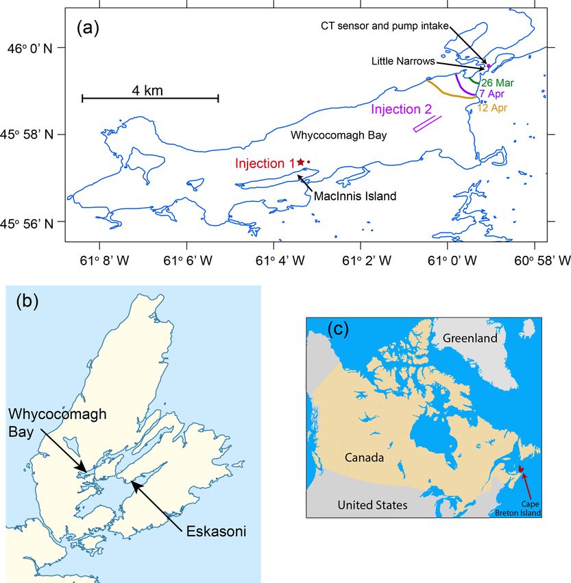
3352                                                     C. C. Manning et al.: Gas exchange and productivity during ice melt

lenging, measurements of productivity and gas exchange are          fraction of autotrophic production available for export to wa-
limited. Biogeochemical time-series observations resolving          ters below the mixed layer. The time-series approach allowed
seasonal changes in productivity are particularly scarce in         us to quantify non-steady-state O2 fluxes, which can be a sig-
the Arctic (MacGilchrist et al., 2014; Stanley et al., 2015).       nificant fraction of the total O2 flux in many regions (Hamme
Measurements at Palmer Station in Antarctica show a strong          et al., 2012; Tortell et al., 2014; Manning et al., 2017b). We
seasonality in biological productivity and carbon uptake as-        quantify GOP with discrete measurements of the triple oxy-
sociated with changes in light, physical mixing, and graz-          gen isotopic composition of O2 (Luz et al., 1999; Luz and
ing, and demonstrate the benefits of high-frequency sampling        Barkan, 2000; Juranek and Quay, 2013) and NOP with near-
for quantifying CO2 uptake in seasonally ice-covered waters         continuous measurements of the O2 /Ar saturation anomaly
(Ducklow et al., 2013; Tortell et al., 2014; Goldman et al.,        (Cassar et al., 2009).
2015).                                                                 To our knowledge, there are no other published field-based
   The parameterization of gas exchange in the presence of          experiments where the dual tracer technique was used in the
ice also remains highly uncertain. Many investigators have          presence of ice, and this study adds to a limited number of in
assumed that there is negligible gas transfer through ice, and      situ measurements of NOP and GOP during ice melt (Gold-
therefore the gas transfer velocity can be linearly scaled as a     man et al., 2015; Stanley et al., 2015; Eveleth et al., 2017).
function of the fraction of open water, multiplied by the open
water gas transfer velocity (Takahashi et al., 2009; Legge          1.1   Site description
et al., 2015; Evans et al., 2015; Stanley et al., 2015). A recent
field study by Butterworth and Miller (2016) in the Southern        The Bras d’Or Lake system consists of several intercon-
Ocean at 0 %–100 % ice cover verified this approach. How-           nected channels and basins and has a total surface area of
ever, other studies report that gas exchange is reduced or en-      1070 km2 and an average depth of ∼ 30 m (maximum 280 m)
hanced in the presence of sea ice relative to a linear scaling      (Petrie and Raymond, 2002; Petrie and Bugden, 2002). The
based on the fraction of open water, including some stud-           Bras d’Or Lake system exchanges water with the Atlantic
ies measuring higher transfer velocities in ice-covered waters      Ocean primarily through the Great Bras d’Or Channel at the
than in open water (Fanning and Torres, 1991; Else et al.,          northeastern region of the estuary; this channel has a shal-
2011; Papakyriakou and Miller, 2011; Rutgers van der Lo-            low (16 m deep) and narrow (0.3 km wide) sill at the mouth
eff et al., 2014). Additional studies show that gas exchange        (Petrie and Raymond, 2002). We conducted the work for this
in ice-covered waters cannot be predicted from wind speed           study in Whycocomagh Bay, an enclosed embayment ap-
alone, which may be a cause of the wide range of results            proximately 13 km long and 3 km wide, at the northwestern
(Loose et al., 2009, 2016; Lovely et al., 2015). An additional      end of the estuary, approximately 60 km from the open ocean
factor reducing air–water exchange in ice-covered waters is         (Fig. 1). Whycocomagh Bay is separated from the rest of the
that ice significantly reduces fetch for wave generation, and       Bras d’Or Lake system by Little Narrows, a channel which
therefore wind-driven near-surface turbulence (Squire et al.,       is approximately 0.2 km wide and 0.5 km long. In Whycoco-
1995; Overeem et al., 2011). However, other processes may           magh Bay, there are two basins (western and eastern basin)
enhance near-surface turbulence in the presence of sea ice          that are up to 40 m deep. Little Narrows channel is ∼ 15–
including convection associated with heat loss and brine re-        20 m deep (Gurbutt and Petrie, 1995). The annual maximum
jection (Morison et al., 1992; Smith and Morison, 1993),            ice cover is typically reached in early March. Ice disappears
boundary layer shear between ice and water (McPhee, 1992;           rapidly during April until its total melt by the first week of
Saucier et al., 2004), and wave interactions with drifting ice      May (Petrie and Bugden, 2002).
(Kohout and Meylan, 2008).                                             The Bras d’Or Lakes system exhibits standard estuarine
   In this study, we measured productivity and gas exchange         circulation with freshwater flowing outward at the surface
over a 1-month period during and following ice melt in              and denser saltwater flowing inward in the deeper layers
Whycocomagh Bay, an estuary in the Bras d’Or Lake sys-              (Gurbutt et al., 1995; Gurbutt and Petrie, 1995). The deep
tem on Cape Breton Island in Nova Scotia, Canada (see               water in western Whycocomagh Bay is strongly isolated due
Sect. 1.1 for a full site description and map). We performed        to the presence of a sill at the bottom of Little Narrows
two dual tracer release experiments at different fractions of       channel, and very little mixing occurs between the surface
ice cover to quantify air–water gas exchange by adding 3 He         and sub-surface waters (Petrie and Bugden, 2002). Whyco-
and SF6 to the mixed layer. We measured net oxygen pro-             comagh Bay receives a relatively large amount of freshwater
duction (NOP) and gross oxygen production (GOP) at Little           compared to other regions of the bay. This freshwater forms
Narrows, while Whycocomagh Bay transitioned from com-               ice in winter and the stratification remains very stable, pre-
pletely ice-covered to ice-free conditions. GOP is the total        venting vertical mixing (Krauel, 1975). In general, exclud-
amount of O2 generated by autotrophic microbes as a result          ing the narrow channels in direct contact with the ocean, the
of photosynthesis. NOP is GOP minus respiratory consump-            Bras d’Or Lakes system does not exhibit significant tidally
tion of O2 by autotrophs and heterotrophs. The NOP/GOP              driven variability in temperature, salinity, and sea surface
ratio provides an estimate of the export efficiency, i.e., the      level (Krauel, 1975; Petrie, 1999; Petrie and Bugden, 2002;

Biogeosciences, 16, 3351–3376, 2019                                                     www.biogeosciences.net/16/3351/2019/
C. C. Manning et al.: Gas exchange and productivity during ice melt                                                                    3353

Figure 1. Map of Whycocomagh Bay and surrounding region. (a) Map of Whycocomagh Bay showing the locations of Injections 1 and 2
and the sampling equipment at Little Narrows. For Injection 1, the injection location is shown with a red star and the location where initial
samples were collected is shown with a red circle. The colored lines labeled 26 March, 7 and 12 April show the location of the ice edge on
these days. (b) Map of Cape Breton Island, showing the location of Whycocomagh Bay and Eskasoni (where wind speeds were obtained).
(c) Map of Canada showing location of Cape Breton Island.

Dupont et al., 2003). A 21 d time series in western Whycoco-             ber 1995 and 30 % at 30 m depth on 23 September 1996,
magh Bay showed no detectable diurnal or semidiurnal tides               and the western basin was persistently anoxic (Strain et al.,
(Dupont et al., 2003).                                                   2001).
   To our knowledge, there are no previously published mea-
surements of water-column chemistry in Whycocomagh Bay
in ice-covered conditions. Measurements from July 1974                   2     Field and analytical methods
showed that the western portion of Whycocomagh Bay be-
came anoxic in the isolated deep waters below 25 m depth,                2.1    Sampling setup at Little Narrows
whereas measurements in the eastern portion of the basin
                                                                         Table 1 presents key events that occurred during the ex-
(closer to Little Narrows) showed the water column had an
                                                                         periment. We continuously sampled water at Little Nar-
O2 saturation of 61 % at the bottom depth of 30 m (Krauel,
                                                                         rows channel (Fig. 1) during a 33 d time series (25 March–
1975; Gurbutt and Petrie, 1995). Measurements collected
                                                                         28 April 2013). We moored a Goulds SB Bruiser 5–18 GPM
from 1995 to 1997 (from late April to late September)
                                                                         submersible pump with intake at ∼ 0.5 m depth (within the
showed O2 concentrations in Whycocomagh Bay from 1 to
                                                                         mixed layer), placed inside a mesh filter bag to prevent large
5 m depth were near equilibrium (94 % to 112 % saturation)
                                                                         particles from clogging the pump, and a conductivity and
throughout the bay. In the deeper waters, O2 concentrations
                                                                         temperature (CT) sensor (Sea-Bird Electronics SBE37) at
in eastern Whycocomagh Bay ranged from 69 % at 25 m
                                                                         ∼ 0.5 m depth. From the submersible pump, water flowed
depth on 28 April 1996 to 54 % at 13 m depth on 26 Septem-
                                                                         through flexible high-pressure PVC tubing submerged un-

www.biogeosciences.net/16/3351/2019/                                                              Biogeosciences, 16, 3351–3376, 2019
3354                                                    C. C. Manning et al.: Gas exchange and productivity during ice melt

derwater to a 3-port pressure-relief valve (on shore) and was      periodically crosses the channel and operates 24 h per day.
then pumped along shore (∼ 50 m) to our sampling appara-           We found no correlations between our temperature, salinity,
tus. The water passed through three 1000 canister filters (100,    and geochemical measurements and the position of the ferry
20, and 5 µm nominal pore size) and then into a sampling           within the channel. We collected conductivity, temperature,
manifold containing valves for distributing water for mea-         and depth (CTD) profiles with a SBE 19Plus sensor at Lit-
surement of O2 /Ar (continuously, by mass spectrometry)            tle Narrows, usually by boat using a winch, but occasionally
and for discrete sampling. As discussed below, we sampled          by lowering the CTD by hand on a rope from the Little Nar-
discretely for SF6 , 3 He, and O2 /Ar and the triple oxygen iso-   rows cable ferry. This CTD package was also equipped with
topic composition of O2 , and near-continuously for O2 /Ar.        an O2 sensor, but unfortunately the O2 sensor malfunctioned
Excess water flowed through tubing back into the bay. We           throughout the experiment. Therefore, we can characterize
covered the tubing on shore and the filter canisters in foam       vertical structure of salinity and temperature but not O2 .
insulation to minimize temperature changes in the water.              The GPS-equipped boat enabled us to map out the location
   We deployed a Nortek acoustic Doppler current profiler          of the ice edge nearest to Little Narrows, to perform the sec-
(ADCP) at ∼ 4 m depth in the middle of the channel from            ond tracer injection, and to sample after the tracer injection.
7 to 28 April. The mean current speed at 0.5 m depth was
3.4 km d−1 (3.9 cm s−1 ) with an orientation toward 31◦ (ap-       2.2   Tracer injections
proximately along the channel axis), indicating the transit
time through Little Narrows is relatively short. The ADCP          The approach in this study was to dissolve the tracer mixture
data are shown in Supplement Fig. S1. Our measurements             (3 He/SF6 ) in Whycocomagh Bay, and sample continuously
(salinity, O2 /Ar, etc.) did not display any correlation with      at Little Narrows, a constriction at the mouth of the bay. The
tidal cycles, consistent with previous studies of the Bras d’Or    net surface flow within Whycocomagh Bay, Little Narrows,
Lakes system indicating tides have a negligible influence on       and St. Patrick’s Channel is toward the ocean due to the sub-
water properties within Whycocomagh Bay (Krauel, 1975;             stantial freshwater inputs to the bay from surface runoff and
Petrie, 1999; Petrie and Bugden, 2002; Dupont et al., 2003).       precipitation (Gurbutt and Petrie, 1995; Yang et al., 2007),
   The CT sensor was initially placed closer to shore than         and therefore tracer dissolved within the bay at the surface
the water pump because the cable was not long enough to            will eventually pass through Little Narrows, or be ventilated
reach the pump, but after obtaining a longer cable, we were        to the atmosphere. Two tracer injections occurred during the
able to co-locate the CT sensor with the water pump (be-           time series, resulting in estimates of the gas transfer veloc-
ginning 12 April). For the discrete samples, we used the CT        ity for two extremes: near-complete ice cover and essentially
sensor temperature and salinity measurements beginning on          ice-free conditions.
12 April (when we moved the CT to the same location as                Injection 1 occurred through a hole in the ice from 30
the pump) to calculate the equilibrium concentration of each       to 31 March, near MacInnis Island (Fig. 1a). Approxi-
gas. Prior to 12 April, we collected measurements with a           mately 0.11 mol SF6 and 4.0 × 10⁻⁴ mol 3 He were diluted
YSI temperature and salinity probe from the water on shore         by a factor of 50 with N2 and then bubbled using a manifold
and used these measurements as the temperature and salinity        within the mixed layer, over a 21 h period. The ice thickness
for the discrete samples. We determined the average warm-          was ∼ 0.3 m and the injection occurred in the upper 0.5 m of
ing through the underway line to be 0.37 ± 0.22 ◦ C based on       the water column. Because the tracer was added at a fixed
comparisons between the temperatures from the CT sensor            location, it was added very slowly to increase the fraction
(in situ) and the YSI probe (on shore) after 12 April and ap-      of the gas that dissolved. We sampled for initial 3 He and
plied this offset to all YSI temperature measurements. For the     SF6 concentrations at the injection site, immediately before
continuous O2 /Ar data we used a temperature record from a         starting the injection, and after terminating the tracer addi-
thermocouple located in the sampling bucket because it had         tion, by drilling several holes > 10 m away from the injec-
fewer gaps in time. We calibrated the thermocouple using an        tion site (because the bubbling action would have perturbed
Aanderaa 4330 optode sensor which contains a temperature           gas concentrations at the injection site). Subsequently, we
sensor (accuracy ±0.03 ◦ C) and then decreased the tempera-        sampled the tracer as it flowed through Little Narrows from
ture by 0.37 ◦ C to correct for warming effects.                   7 to 11 April. From 31 March to 11 April, the bay was
   We installed the gas chromatograph (for measurement of          nearly completely full of ice, with a small opening near Lit-
SF6 ) and mass spectrometer (for measurement of O2 /Ar) in-        tle Narrows (Fig. 1a). We also collected under-ice samples
side a garage connected to the Little Narrows Ferry building.      for O2 /Ar and O2 triple oxygen isotope (TOI) composition
The majority of the wet equipment was set up outside the           immediately before and after the injection but they displayed
garage adjacent to a window on the garage, which was used          a wide range in values for O2 /Ar, from −14 % to 2 %. There-
for connecting equipment and power cables between the out-         fore, we were unable to define any initial under-ice values for
doors and indoors.                                                 these parameters.
   We deployed the water pump and in situ CT sensor to                Injection 2 occurred by boat on the morning of 19 April.
the east (oceanward) of the Little Narrows cable ferry which       By this time, the bay was nearly ice-free and all tracer from

Biogeosciences, 16, 3351–3376, 2019                                                    www.biogeosciences.net/16/3351/2019/
C. C. Manning et al.: Gas exchange and productivity during ice melt                                                         3355

Table 1. Key events during experiment

                             Date (in 2013)   Event
                             22 Mar           First CTD profile at Little Narrows
                             25 Mar           Start of continuous water sampling with water pump
                                              and CT sensor at Little Narrows
                             30–31 Mar        Tracer Injection 1 (under ice)
                             7 Apr            ADCP installed at Little Narrows
                             7–10 Apr         Tracer from Injection 1 sampled at Little Narrows
                             16–19 Apr        Rapid decline in ice cover in Whycocomagh Bay
                             19 Apr           Tracer Injection 2 (open water)
                             20–23 Apr        Tracer from Injection 2 sampled at Little Narrows
                             28 Apr           End of continuous water sampling and ADCP measurements
                                              at Little Narrows, and last CTD profile at Little Narrows

the previous experiment had passed through and/or been ven-         Barkan and Luz (2003) with modifications as described in
tilated to the atmosphere such that the tracer concentrations       Stanley et al. (2010, 2015).
at Little Narrows were below detection. While the boat was             The precision of the discrete samples, calculated based
moving, we used the same manifold as for Injection 1 to bub-        on the standard deviation of equilibrated water samples run
ble approximately 4.4 mol SF6 and 0.021 mol 3 He, diluted           daily along with the environmental samples was 0.011 and
by a factor of four with N2 into the mixed layer (Fig. 1a).         0.020 ‰ for δ 17 O and δ 18 O, respectively, 5.6 per meg for
The injection lasted 40 min. We detected the tracers at Lit-        17 1, and 0.07 % for O /Ar. The mean difference between the
                                                                                           2
tle Narrows beginning on 20 April 23:30 UTC and measured            EIMS and discrete samples was 0.05 %, and the mean mag-
the change in the ratio between 20 and 23 April as the tracer       nitude of the difference was 0.35 %; given the small mean
patch flowed through Little Narrows. We used a higher quan-         offset, the EIMS data were not calibrated using discrete sam-
tity and concentration of SF6 and 3 He during this injection        ples.
because we expected the tracer would be ventilated more
rapidly due to higher gas exchange rates given the open wa-         2.4   Measurement of SF6
ter conditions. We were able to inject the tracer more rapidly
because it was distributed over a large area instead of through     For SF6 , we collected ∼ 20 mL of water in 50 mL glass gas-
a small hole in the ice.                                            tight syringes, then added ∼20 mL of nitrogen and allowed
                                                                    the samples to be shaken for 10 min to achieve equilibration
                                                                    between the headspace and water (Wanninkhof et al., 1987).
2.3   Measurement of O2 /Ar and the triple oxygen                   After the water equilibrated to room temperature, we injected
      isotopic composition of O2                                    1 mL of the headspace into an SRI-8610C gas chromatograph
                                                                    with an electron capture detector, heated to 300 ◦ C (Lovely
                                                                    et al., 2015). We calibrated the detector response using a 150
We set up an equilibrator inlet mass spectrometer (EIMS)
                                                                    parts per trillion SF6 standard (balance N2 ).
for measurement of O2 /Ar similarly to the system described
                                                                       We also operated an automated gas extraction system at
in Cassar et al. (2009). However, we used a larger mem-
                                                                    Little Narrows which sampled nearly every hour. The sys-
brane contactor cartridge (Liqui-Cel MiniModule 1.7 × 5.5)
                                                                    tem recirculated a 118 mL loop of water through a membrane
because the design is more robust than the Liqui-Cel Micro-
                                                                    contactor, and the headspace of the membrane contactor was
Module 0.75×1 used by Cassar et al. (2009). The water flow
                                                                    under vacuum, causing the dissolved gas to be extracted from
rate through the cartridge was ∼ 1.5 L min−1 . We attached a
                                                                    the water into the headspace. When the automated system
custom female Luer-Lok fitting paired to a capillary adapter
                                                                    showed measurable SF6 in the water, we began collecting
to the upper headspace sampling port and the lower sampling
                                                                    discrete samples for SF6 and 3 He.
port was left closed.
                                                                       SF6 equilibrium solubility concentrations are calculated
   For O2 /Ar and the triple oxygen isotopic composition
                                                                    following Bullister et al. (2002) and diffusivity is from King
of O2 , we collected samples in pre-evacuated, pre-poisoned
                                                                    and Saltzman (1995). Precision of the system, based on the
glass flasks from a spigot in the water pumped to shore, or for
                                                                    standard deviation of measurements of the 150 ppt standard,
shipboard sampling, using a small submersible water pump.
                                                                    was 7 %. We assume a dry atmospheric mole fraction of 8 ppt
Analysis occurred within ∼ 6 months of flask evacuation and
                                                                    for SF6 (Bullister, 2015).
4 months of sample collection at the Woods Hole Oceano-
graphic Institution with a Thermo Fisher Scientific MAT 253
isotope ratio mass spectrometer, following the method of

www.biogeosciences.net/16/3351/2019/                                                       Biogeosciences, 16, 3351–3376, 2019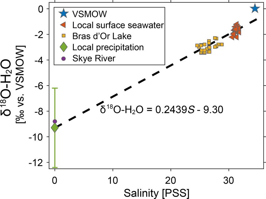
3356 C. C. Manning et al.: Gas exchange and productivity during ice melt
2.5 Measurement of 3 He ing the time series (Fig. 3). From 25 March through 8 April
the water column was strongly stratified and we estimated
For 3 He analysis, we collected samples in copper tubes, the mixed layer depth to average 0.8(0.3) m. During this pe-
mounted in aluminum channels and sealed the samples at riod, it was often difficult to determine the exact mixed layer
each end using clamps. Sample analysis occurred at the depth because the mixed layer depth was similar to the length
Lamont Doherty Earth Observatory, using a VG5400 mass of the CTD instrument and obtaining a stable CTD response
spectrometer for 3 He and 4 He concentration (Ludin et al., so close to the surface was challenging. Following 8 April,
1998). Error for 3 He sample analysis (combined precision the mixed layer deepened and warmed and its salinity in-
and accuracy) was ≤ 2 % of the measured 3 He-excess con- creased, likely due to convection and heating following sea
centration above equilibrium. We used He solubility from ice melt. For this period, we defined the mixed layer depth as
Dempsey E. Lott III and William J. Jenkins (personal com- the first depth where the density is 1 kg m−3 greater than the
munication, 2015) and diffusivity from Jähne et al. (1987a). value at 1 m. The mixed layer reached a maximum of 3.0 m
The Lott and Jenkins solubility values are ∼ 2 % higher on 23 April and then shoaled by the end of the time series on
than published data from Weiss (1971). The He solubility 28 April. On most days, the density profile and mixed layer
is for bulk He and we calculate the 3 He solubility using depth were driven by stratification in salinity, but for the final
an atmospheric mole ratio M(3 He)/M(4 He) = 1.399×10⁻⁶ profile on 28 April the mixed layer depth was determined by
(Mamyrin et al., 1970; Porcelli et al., 2002), although some a combination of temperature and salinity stratification due
more recent results indicate the current ratio may be slightly to heat uptake by the surface water following the ice melt.
lower, ' 1.390 × 10⁻⁶ (Brennwald et al., 2013). We use the These changes in mixed layer depth must be considered in
He equilibrium isotopic fractionation as described in Benson order to interpret the O2 measurements and to quantify the
and Krause (1980b). gas transfer velocity.
3.2 Gas transfer velocity
3 Calculations, results, and discussion
3.2.1 Calculation
The three goals of the experiment were to (1) quantify gas
transfer velocity by dual tracer release, (2) quantify gross We calculate the gas transfer velocity using the dual tracer
oxygen production from the triple isotopic composition of approach (Watson et al., 1991; Wanninkhof et al., 1993). For
O2 , and (3) quantify net oxygen production from O2 /Ar. We each experiment, we dissolved a mixture of 3 He and SF6 in
begin by discussing the hydrographic characteristics of the the water, both of which are normally present at very low am-
study area and then describe the calculations, results, and in- bient concentrations, and then measured the change in the ra-
terpretation for each of the three goals, in sequence. tio of the two gases as a function of time. Measuring two trac-
ers enables correction for dilution and mixing, which reduces
3.1 Hydrography the excess concentrations of both gases (relative to air–water
equilibrium) but does not change their ratio. Over time, the
We began sampling O2 at Little Narrows on 25 March, when
concentrations of both gases decay toward air–water equi-
Whycocomagh Bay was nearly (> 95 %) fully covered by
librium as gas is ventilated to the atmosphere through gas
ice, and completed sampling on 28 April, when the bay was
exchange. Because the molecular diffusivity of 3 He is 8–
completely ice-free (Fig. 2). The surface ice cover retreated
9 times higher than SF6 , 3 He is lost to the atmosphere more
most rapidly between 16 and 18 April and was completely
rapidly than SF6 , and therefore the 3 He:SF6 ratio decreases
gone by 22 April or perhaps even earlier. Figure 2 shows
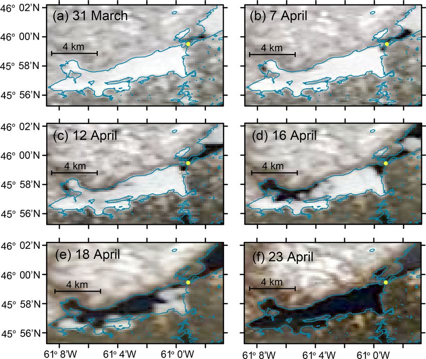
with time. The ratio of the gas transfer velocity for the two
18 April and 23 April; MODIS satellite images on 22 April
gases is expressed as
were also ice-free (but more blurry, and so are not shown in
the figure) and we estimated ice cover to be < 10 % in the Sc3 He −n
k3 He
bay during surveys by boat during daytime on 20 April. The = , (1)
kSF6 ScSF6
ice was likely melting even at the beginning of the time se-
ries since the surface water temperature was always above where k is the gas transfer velocity (m d−1 ) and Sc is the
the freezing temperature of water (Fig. 3). Changes in sur- Schmidt number (unitless), defined as the kinematic viscos-
face ice cover and total ice volume are both important factors ity of water divided by the molecular diffusivity of the gas in
during the study; changes in ice volume/thickness will af- water, and n is an empirical exponent, typically between 0.5
fect stratification and convection in the mixed layer as well and 0.67 (Jähne et al., 1984; Liss and Merlivat, 1986). Us-
as light penetration through the ice, and the surface ice cover ing a time series of measurements of the two gases, the gas
affects the rate of gas exchange (Smith and Morison, 1993; transfer velocity for 3 He is calculated as
Butterworth and Miller, 2016; Loose et al., 2016). !
d ln 3 He exc /[SF6 ]exc
CTD profiles at Little Narrows channel near the water k3 He = h . (2)
dt 1 − ScSF6 /Sc3 He −n
pump intake showed substantial changes in stratification dur-
Biogeosciences, 16, 3351–3376, 2019 www.biogeosciences.net/16/3351/2019/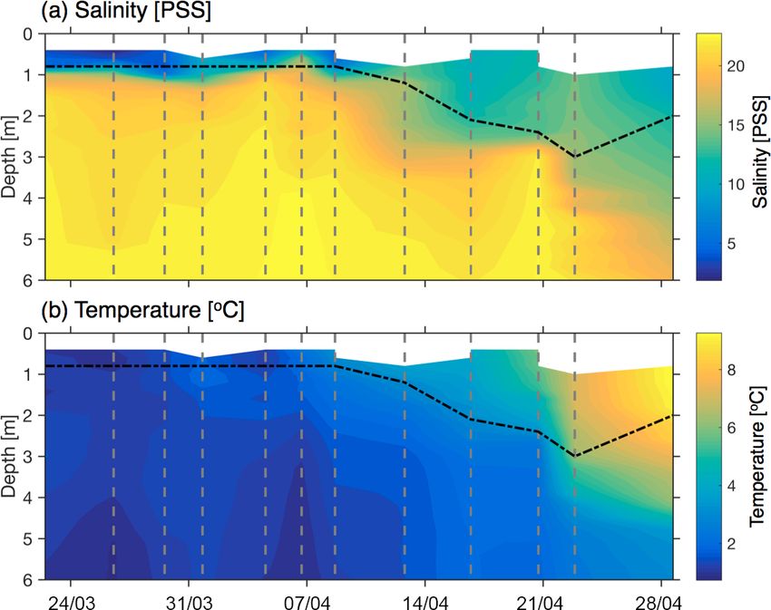
C. C. Manning et al.: Gas exchange and productivity during ice melt                                                                  3357

Figure 2. Satellite images showing changes in ice cover in Whycocomagh Bay. MODIS Terra true color images showing changes ice cover
during the time series between 31 March and 23 April. Little Narrows is indicated with a yellow circle in all images. Ice cover retreated
most rapidly between 12 and 20 April. Shoreline data (blue lines) are from GeoGratis/Natural Resources Canada (http://geogratis.gc.ca, last
access: 27 August 2019) and satellite data are from NASA Worldview (http://worldview.earthdata.nasa.gov, last access: 27 August 2019).

Here h is the mixed layer depth, [3 He]exc = [3 He]meas −               For this study, we use a Schmidt number dependence of
[3 He]eq where [3 He]exc is the 3 He-excess concentration,              n = 0.5 which is appropriate for wavy, unbroken water sur-
[3 He]meas is the measured concentration, and [3 He]eq is the           faces (no bubble entrainment) (Jähne et al., 1984, 1987a; Liss
equilibrium concentration (calculated as a function of tem-             and Merlivat, 1986; Ho et al., 2011b). At Little Narrows, we
perature and salinity). [SF6 ]exc is defined analogously.               observed that tidal currents generated surface waves, even at
   We can write the analytical solution to Eq. (2) as (Ho et al.,       low wind speeds. These waves produce near-surface water
2011b)                                                                  turbulence which is the ultimate driver of air–water gas ex-
                                                                        change (Jähne et al., 1987b; Wanninkhof et al., 2009).
    [3 He]exc      [3 He]exc                                               The Schmidt number at a salinity of 4 PSS and temper-

                    =                                                   ature of 2 ◦ C is 305 for 3 He and 2684 for SF6 . The initial
    [SF6 ]exct     [SF6 ]exc t−1
                   "               #!                                  ScSF6 /Sc3 He ratio was 8.7 for Injection 1 and 8.2 for Injec-
                           ScSF6 −n

          k3 He 1t                                                      tion 2.
    exp −            1−                .                       (3)
               h           Sc3 He
                                                                        3.2.2   Results
Using this equation and a cost function, we can find the value
of k3 He that minimizes the error between the measured and              The gas transfer velocity was much lower for Injection 1,
modeled [3 He]exc / [SF6 ]exc . Once k3 He is known, we can cal-        which was sampled while the basin was essentially full of
culate k for any other gas using Eq. (1) by substituting ScSF6          ice (31 March–10 April), compared to Injection 2, which was
for the Schmidt number of the gas of interest. For example,             sampled when the basin was nearly ice-free (20–23 April).
for Sc = 600 (the Schmidt number for CO2 at 20 ◦ C in fresh-            We used Eq. (3) to model the measurements. We started the
water),                                                                 model at the time of the first measurement, initialized it with
                                                                        an initial excess concentration ratio and ran it through time
                            −n
                     600                                                for the duration of the injection. We selected the value of k3 He
k600 = k3 He                       .                           (4)      yielding the smallest root mean square deviation (RMSD) be-
                    Sc3 He

www.biogeosciences.net/16/3351/2019/                                                            Biogeosciences, 16, 3351–3376, 2019
3358 C. C. Manning et al.: Gas exchange and productivity during ice melt
Figure 3. Temperature and salinity profiles at Little Narrows. (a) Salinity and (b) temperature profiles measured at Little Narrows. The
vertical grey dashed lines indicate the timing of CTD casts (22, 26, 29, and 31 March, and 4, 6, 8, 12, 16, 20, 23, and 28 April). The black
dot-dashed line shows the estimated mixed layer depth. The data in this plot were binned into 0.2 m depth bins from 0.4 to 3.0 and 0.3 m
depth bins from 3.3 to 9.9 m. The shallowest depth varies between casts due to challenges in getting stable CTD data in the upper 1 m.
tween the measured ratio and modeled ratio for each injec-
tion. The model ran 1000 times using a Monte Carlo simula-
tion where the measured excess concentration ratios, includ-
ing the initial condition, are varied with a Gaussian distri-
bution, with the standard deviation being the estimated mea-
surement error in the ratio (7.3 %).
We assume a constant Sc3 He /ScSF6 and mixed layer depth
(h) for each injection. In actuality, during each injection
Sc3 He varies by ∼1 % and the ratio of the Schmidt numbers
varies by less than 0.2 %, so this is a small source of error. For
Injection 1, we assume a mixed layer depth (h) of 0.8(0.3) m.
This depth is consistent with the salinity profiles at Little
Narrows (Fig. 3a) between 31 March and 8 April (between
0.6 and 1.0 m depth), as well as measurements with a hand-
held temperature probe at the site of Injection 1 which indi-
cated that the mixed layer depth was between 0.75 and 1 m.
The mixed layer depth may have increased slightly between
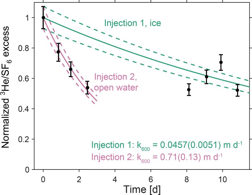
Figure 4. Measured and modeled excess tracer ratios. Measured and
8 and 10 April, but was likely 1.3 m or less (Fig. 3).
modeled ratio of excess 3 He/SF6 , normalized to the initial mea-
For Injection 1, the excess SF6 and 3 He concentrations sured ratio for each injection. The modeled excess ratio is calcu-
were reduced by 2 orders of magnitude by the time the lated using the k3 He that minimizes error between the model and
tracer reached Little Narrows (7–11 d after injection). The measurements. Model results are shown for the model initialized
tracer ratio did not display a consistent decrease over the 3 with the initial measured concentration (solid lines), and starting 1
days we sampled it at Little Narrows, which may be due to standard deviation above or below the measured initial concentra-
the substantially lower gas transfer velocity, as well as the tion (based on an error of 7.3 % in the tracer ratio, dashed lines).
very low tracer concentrations potentially increasing mea-
Biogeosciences, 16, 3351–3376, 2019 www.biogeosciences.net/16/3351/2019/C. C. Manning et al.: Gas exchange and productivity during ice melt 3359
Table 2. Data for determination of the gas transfer velocity.
Injection 1
Date Time Salinitya Temperaturea δ 3 Heb [SF6 ] [3 He]exc / [SF6 ]exc
(ADT) (PSS) (◦ C) (%) (mol L−1 ) (mol mol−1 )
31 Mar 15:00 0.9 2.1 17176 66.6 0.00788
7 Apr 18:00 13.2 2.6 13.8 0.152 0.00411
8 Apr 17:27 8.4 2.0 56.9 0.423 0.00480
9 Apr 12:47 9.0 2.1 39.0 0.289 0.00553
10 Apr 11:02 9.3 1.8 12.6 0.115 0.00405
Injection 2
Date Time Salinitya Temperaturea δ 3 Heb [SF6 ] [3 He]exc / [SF6 ]exc
(ADT) (PSS) (◦ C) (%) (mo L−1 ) (mol mol−1 )
20 Apr 23:30 11.18 5.64 310.3 3.96 0.00227
21 Apr 20:00 14.91 6.49 91.8 1.60 0.00176
22 Apr 12:27 14.64 7.16 43.6 0.938 0.00150
23 Apr 10:40 11.01 5.73 6.5 0.299 0.000799
a During Injection 1, we measured temperature and salinity with a YSI probe to a precision of one decimal place. During
Injection 2, we measured temperature with a calibrated thermocouple and salinity with the in situ CTD, to a precision of
two decimal places. b δ 3 He = ((3 He/4 He)meas /(3 He/4 He)eq ).
surement uncertainty. The best fit to all the measurements in a gas transfer velocity that is 8 % lower in the presence
was k600 = 0.0457(0.0051) m d−1 , in the presence of ice and of ice (for Injection 1) and 0.4 % lower in open water (for
a shallow mixed layer, with the uncertainty the standard de- Injection 2).
viation of the distribution of k600 from the Monte Carlo sim-
ulation (Fig. 4). 3.2.3 Discussion
The mixed layer appeared to deepen between the CTD
profiles on 8 April 16:08 UTC and 12 April 19:13 UTC The gas transfer velocity calculated for Injection 1 is the ef-
(Fig. 3), and it is possible that the mixed layer depth on 9– fective gas transfer velocity (keff ); it averages the gas transfer
10 April may have been slightly deeper than the estimate velocity through ice (kice ), weighted by the time the tracer
of 0.8(0.3) m. However, if mixed layer deepening had a sig- spent under ice, and the gas transfer velocity for open wa-
nificant influence on our gas transfer velocity estimate, we ter (k), weighted by the time the tracer spent in open water
would expect k600 (calculated assuming a constant mixed (Loose et al., 2014). In partially ice-covered waters, the ef-
layer depth) to be lowest when calculated over the longest fective gas transfer velocity is sometimes calculated as
time period, using the sample collected on 10 April. Instead, keff = (f )k + (1 − f )kice , (5)
the gas transfer velocity was actually the lowest when inte-
grated to 9 April (the excess tracer ratio appears above the where f is the fraction of open water (Loose et al., 2014;
best-fit line) and second lowest on 8 April. Since the gas Lovely et al., 2015). If kice is negligible, then keff = (f )k
transfer velocities for Injection 1 integrate over 7–10 d, any (Loose and Jenkins, 2014; Crabeck et al., 2014; Butterworth
change in mixed layer depth during the last 1–2 d will have a and Miller, 2016). For Injection 2, we determined k, the value
small effect on the calculated k. for open water. We expect kice to be lower than k because the
For Injection 2, we use a mixed layer depth of 2.7(0.3) m ice acts as a physical barrier to gas exchange. The rate of
based on CTD profiles at Little Narrows on 20 and 23 April, gas molecular diffusion in water (Jähne et al., 1987a; King
which had mixed layer depths of 2.4 and 3.0 m, respectively and Saltzman, 1995) is higher than gas diffusion through ice
(Fig. 3a). Calculation of the gas transfer velocity for Injec- (Gosink et al., 1976; Ahn et al., 2008; Loose et al., 2011b;
tion 2 was relatively straightforward as the ratio of excess Lovely et al., 2015). However, the exact rate of gas diffusion
3 He/SF steadily decreased over the five measurements (Ta-
6 through saltwater ice (and by extension the value of kice ) is
ble 2). The best fit to all four measurements was k600 = not well constrained and likely varies based on the physical
0.71(0.13) m d−1 for open water (Fig. 4). properties of the ice such as brine volume and temperature
Using the published He solubility from Weiss (1971) in- (Golden et al., 2007; Loose et al., 2011b; Zhou et al., 2013;
stead of the unpublished data of Dempsey E. Lott III and Moreau et al., 2014; Lovely et al., 2015).
William J. Jenkins (personal communication, 2015) results To evaluate these results within the framework of Eq. (5),
we must estimate the fractional ice cover during Injection 1.
www.biogeosciences.net/16/3351/2019/ Biogeosciences, 16, 3351–3376, 20193360 C. C. Manning et al.: Gas exchange and productivity during ice melt Visual surveys along the shoreline of Whycocomagh Bay and 0.71(0.13) m d−1 from 21 April until the end of the time se- satellite data indicated that the bay was nearly fully covered ries on 28 April. Surveys by boat on 19 and 20 April indi- with a continuous sheet of ice from 31 March to 10 April, ex- cated < 10 % ice cover on these days, and we collected the cept for an opening close to Little Narrows (Fig. 2a–b). Be- first tracer measurements following Injection 2 on 20 April ginning between 7 and 12 April, a small region of water ap- 23:30 UTC. Between 16 and 20 April, we apply a linear in- peared to open up along the shoreline northwest of the site of terpolation of the k600 for Injection 1 and Injection 2 as a Injection 1; however, by this time the tracer patch had moved function of time. The gas transfer velocity is most uncertain eastward close to Little Narrows and likely was not signif- during the period when the ice cover rapidly decreased be- icantly affected by this open water (Fig. 2c). We mapped cause we do not have any measurements of gas transfer at out the location of the ice edge closest to Little Narrows by intermediate ice cover. However, because the ice cover re- boat on 26 March and 7 and 12 April (Fig. 1a). Using these treated rapidly, only 4 days of the productivity estimates (out surveys and shoreline data, we calculate that for the surface of a 33 d time series) are affected by the uncertainties in gas area of the bay between the injection site and Little Narrows, transfer at intermediate ice cover. f = 0.01 on 26 March, 0.05 on 7 April, and 0.08 on 12 April. The f experienced by the tracer patch during Injection 1 is 3.2.4 Comparison with other estimates likely between 0.02 and 0.08 because the tracer was injected on 30–31 March and flowed through the open water near Lit- To compare the gas exchange estimates with other published tle Narrows between 6 and 11 April. If k for open water is the studies, we use wind speed data measured at 10 m height same for both injections (k = 0.71 m d−1 ), then the results (u10 ) at Eskasoni Reserve, 27 km northeast of Little Nar- yield keff = (f )k with f = 0.064, which is consistent with rows (Fig. 1b) and archived by the Government of Canada the fraction of open water we estimate for Injection 1. Thus (http://climate.weather.gc.ca, last access: 27 August 2019). we conclude that kice was negligible, compared to k. For ex- The archived data are 2 min averages measured once per ample, if kice was even 10 % of k for open water, then keff for hour. During the period that samples with tracer from Injec- Injection 1 would have been ∼ 0.11 m d−1 , more than dou- tion 2 were collected (between 20 April 23:00 and 23 April ble the observed value of 0.0457(0.0051) m d−1 . One source 11:00), the average wind speed was 2.6(1.4) m s−1 and the of uncertainty in estimating the correct value of f is that the median was 2.2 m s−1 . The calculated k600 over this time transit speed between the injection site and Little Narrows period from dual tracer data is 0.71(0.13) m d−1 . Cole and was non-constant. The mean current velocity at Little Nar- Caraco (1998) found k600 = 0.636(0.029) m d−1 (95 % con- rows channel was 3.4 km d−1 , but the tracer took approxi- fidence interval) and their estimate is independent of wind mately 8 d to flow 7 km from the injection site to Little Nar- speed in a lake with daily wind speeds of 1.39(0.06) m s−1 rows. (95 % confidence interval); this k600 is consistent within un- In calculating GOP and NOP by oxygen mass balance, certainty with the Injection 2 result. Standard open ocean we apply the tracer-based gas transfer velocities estimated parameterizations that use a quadratic dependence on wind by dual tracer release throughout the time series, since there speed predict k600 ' 0.5–0.6 m d−1 with uncertainties of ∼ is no consensus on the best treatment of gas transfer in lakes 20 % or ∼ 0.10 m d−1 (Ho et al., 2006; Sweeney et al., 2007; and estuaries (Clark et al., 1995; Cole and Caraco, 1998; Cru- Wanninkhof, 2014). sius and Wanninkhof, 2003; Ho et al., 2011a), nor on the Crusius and Wanninkhof (2003) found that in a lake gas parameterization of gas transfer in the presence of ice (Else exchange can be estimated nearly equally well using three et al., 2011; Lovely et al., 2015; Butterworth and Miller, different parameterizations. Using their parameterizations 2016). Additionally, if bottom-derived turbulence (e.g., from with the wind speed record during our time series, we cal- tidal flow) is a significant contributor to air–water gas ex- culate transfer velocities of 0.32–0.66 m d−1 , and the veloc- change, a parameterization based on wind speed alone may ity is most similar to our result when we use a constant gas not be appropriate. This method of calculating one average transfer velocity k600 = 0.24 m d−1 for u10 < 3.7 m s−1 and k600 for each injection does not enable the development of a k600 = 1.23u10 − 4.30 for u10 ≥ 3.7 m s−1 . However, Cru- wind speed-dependent parameterization for the gas transfer sius and Wanninkhof (2003) parameterized the gas transfer velocity. using instantaneous (e.g., 1 min averaged) winds measured Because the k600 values for Injection 1 and Injection 2 are throughout the time series, not once per hour, and empha- very different, the treatment of the gas transfer velocity in be- size the importance of including the variability in short-term tween the two injections strongly affects the productivity es- winds when quantifying gas exchange at low wind speeds. timates for this period. We use k600 = 0.0457(0.0051) m d−1 If gas transfer velocity has a nonlinear dependence on wind from the beginning of the time series until the end of speed, then short-term wind speed measurements will more 15 April. Figure 2d, collected on 16 April, is the first satel- accurately represent the gas transfer than wind speed val- lite image showing substantial open water within Whyco- ues averaged over longer periods (Livingstone and Imboden, comagh Bay, but the open water is primarily in the west- 1993; Crusius and Wanninkhof, 2003). Since we only have ern half of the bay, far from Little Narrows. We use k600 = 2 min averages measured once per hour (for a total of 60 Biogeosciences, 16, 3351–3376, 2019 www.biogeosciences.net/16/3351/2019/
C. C. Manning et al.: Gas exchange and productivity during ice melt                                                            3361

measurements during Injection 2), the wind record we use           18 O  (i.e., λ=17 /18 , where  is the isotopic fractionation of
may not fully represent the variability in winds during the        O2 due to respiratory consumption) (Luz and Barkan, 2005).
Injection 2 measurement period.                                    This value for λ is selected so that 17 1 is nearly unaffected by
   A source of error in comparisons with published results         respiratory O2 consumption and reflects the proportion of O2
is that the wind speed data come from a different location         that is derived from photosynthesis relative to air–water gas
than the study area. Although Eskasoni Reserve is adjacent to      exchange (Hendricks et al., 2005; Juranek and Quay, 2013;
the Bras d’Or Lake, the local topography and bathymetry are        Nicholson et al., 2014). We report 17 1 in per meg (1 per
different near the reserve and in Whycocomagh Bay. Thus,           meg = 0.001 ‰) due to the small range of values in natural
it is likely that the wind speed and momentum stress at the        waters, typically 8–242 per meg (Juranek and Quay, 2013;
air–water interface differ at Whycocomagh Bay compared to          Manning et al., 2017a).
Eskasoni Reserve (Ortiz-Suslow et al., 2015).                         Two key constraints in the calculation of GOP from mea-
   The measurements are in agreement with other studies            surements of the triple isotopic composition of O2 are the
showing that gas transfer velocity is significantly reduced        isotopic composition of O2 derived from air–water exchange
under near-complete ice cover (Lovely et al., 2015; Butter-        and the isotopic composition of photosynthetic O2 . The com-
worth and Miller, 2016) and contrast with studies showing          position of photosynthetic O2 is dependent on the triple oxy-
enhanced gas transfer under > 85 % ice cover (Fanning and          gen isotopic composition of H2 O, the substrate for photo-
Torres, 1991; Else et al., 2011). We find that keff = (f )k for    synthetic O2 , and the isotopic fractionation associated with
> 90 % ice cover, but we cannot evaluate whether the same          photosynthetic O2 production. In oceanic studies, a common
equation holds at intermediate ice cover because there was         assumption is that the H2 O isotopic composition is equiva-
no injection at a lower fractional ice cover. In this study, the   lent to VSMOW (standard mean ocean water), but in brack-
ice cover was near-continuous across the entire bay during         ish systems it is necessary to estimate the isotopic composi-
Injection 1 and likely did not contain the ice leads that are      tion of water and incorporate this into the GOP calculation
common in Arctic and Antarctic sea ice; differences in gas         (Manning et al., 2017a).
transfer behaviour are expected based on the nature of the            Because we did not measure the triple oxygen isotopic
ice pack.                                                          composition of H2 O, we use previously published measure-
                                                                   ments of δ 18 O-H2 O and published relationships between
3.3     Gross oxygen production                                    δ 17 O-H2 O and δ 18 O-H2 O (Luz and Barkan, 2010; Li and
                                                                   Cassar, 2016) to estimate the values of δ 18 O-H2 O and δ 17 O-
3.3.1     Calculation                                              H2 O during the time series, as described in Manning et al.
                                                                   (2017a). We assume that the waters in the estuary repre-
The triple oxygen isotopic composition of O2 is an effective
                                                                   sent a mixture of two endmembers: seawater and meteoric
tracer of gross photosynthetic O2 production (Juranek and
                                                                   (precipitation-derived). We define the salinity and δ 18 O-H2 O
Quay, 2013). Due to reactions in the upper atmosphere that
                                                                   for the two endmembers and then calculate δ 18 O-H2 O for
impart a small mass-independent isotopic signature on at-
                                                                   each water sample collected during the time series as a linear
mospheric oxygen, dissolved O2 derived from air–water ex-
                                                                   function of salinity. A similar approach is applied for δ 17 O-
change has a unique triple isotopic signature compared to O2
                                                                   H2 O.
generated by photosynthesis and O2 consumed by respira-
                                                                      For the seawater endmember, we use compilations of
tion. We characterize the oxygen isotopic composition using
                                                                   δ 18 O-H2 O and salinity (Schmidt, 1999; Bigg and Rohling,
δ 18 O = X18 /Xstd
               18
                   − 1,                                     (6)    2000) available from an online database (Schmidt et al.,
                                                                   1999). We included all 19 near-surface samples (< 5 m
and express the δ 18 O in ‰ by multiplying by 1000.                depth) between 44–48◦ N and 58–64◦ W in the database. For
Here X 18 = r(18 O/16 O) is the measured ratio and Xstd  18 =      these samples, the average δ 18 O-H2 O = −1.68(0.26) ‰ and
  18    16
r( O/ O)std is the ratio of the isotopes in the standard. We       salinity = 31.25(0.30) PSS.
calculate δ 17 O analogously. For GOP studies, O2 in air is           For the meteoric water endmember, we use an 8-year
the standard for isotopic measurements of O2 and isotopes of       time series of δ 18 O-H2 O measured in Truro, Nova Sco-
H2 O are referenced to the VSMOW-SLAP scale. For clarity,          tia (200 km southwest of our study area and at 40 m el-
we distinguish between the isotopic composition of the two         evation), and archived in the Global Network of Isotopes
substrates (O2 and H2 O) as δ 18 O-O2 and δ 18 O-H2 O.             in Precipitation (GNIP) database (IAEA/WMO, 2016). The
   The term 17 1 quantifies the triple isotopic composition of     amount-weighted value of δ 18 O-H2 O over the time se-
dissolved O2 :                                                     ries was −9.3(3.1) ‰ versus VSMOW, using precipitation
                                                                   measurements from Truro, NS, over the same time pe-
17
     1 = ln(δ 17 O-O2 + 1) − λ ln(δ 18 O-O2 + 1).           (7)    riod from the Government of Canada historical weather
                                                                   database (http://climate.weather.gc.ca, last access: 27 Au-
We report 17 1 with λ = 0.5179, the ratio of the fractiona-        gust 2019). Also, Timsic and Patterson (2014) measured
tion factors for respiratory O2 consumption in 17 O relative to    δ 18 O-H2 O = −8.8(0.1) ‰ on a water sample collected in

www.biogeosciences.net/16/3351/2019/                                                       Biogeosciences, 16, 3351–3376, 2019
3362 C. C. Manning et al.: Gas exchange and productivity during ice melt
at sufficient accuracy to resolve the small excess (Luz and
Barkan, 2010; Li et al., 2015). To calculate the freshwater
and seawater endmembers for δ 17 O-H2 O, we use the aver-
age values of 17 O-excess of 33 per meg for meteoric water
and −5 per meg for seawater (Luz and Barkan, 2010). The
endmembers are δ 17 O-H2 O = −4.888 ‰ and −0.908 ‰ for
meteoric water and seawater, respectively, and the linear re-
gression is δ 17 O-H2 O = 0.1274S − 4.89. These δ values for
H2 O, referenced to VSMOW, are subsequently referenced to
atmospheric O2 using results from Barkan and Luz (2011).
In this study, the choice of δ 18 O-H2 O is more important than
the 17 O-excess because 17 O-excess varies by less than 0.1 ‰
between samples, whereas the freshwater δ 18 O-H2 O differs
from VSMOW by 9.1 ‰. We discuss the sensitivity of the
Figure 5. δ 18 O-H2 O regression versus salinity. Measurements of
δ 18 O-H2 O in local surface seawater, the Bras d’Or Lake, local GOP calculations to the assumed 17 O-excess and δ 18 O-H2 O
precipitation, and the Skye River (within the Whycocomagh Bay below, and the effect of other processes on the isotopic com-
watershed). The regression is calculated using the local precipita- position of H2 O in Sect. 3.6.
tion and seawater values. The local precipitation value is plotted as We calculate GOP using Eq. (7) from Manning et al.
9.3(3.1) ‰, with the error bar the standard deviation of the amount- (2017a), which is equivalent to Eq. (S8) from Prokopenko
weighted annual average. et al. (2011),
X17 −Xeq
17 X18 −Xeq
18
July 2009 from the Skye River, within the Whycocomagh −λ
X17 X 18
Bay watershed (Parker et al., 2007), consistent with the aver- GOP = kO2 [O2 ]eq
age Truro, NS, value. Xp17 −X 17 Xp18 −X18
X17
−λ X 18
Using the two endmembers, S = 0 PSS, δ 18 O-
H2 O = −9.3 ‰ (local meteoric water) and S = 31.25 PSS, 17
h[O2 ] ∂ ∂t1
δ 18 O-H2 O = −1.68 ‰ (local seawater), we derive the + . (9)
equation δ 18 O-H2 O = 0.2439S −9.30 (Fig. 5). This equation Xp17 −X17 X 18 −X 18
X 17
− λ pX18
is consistent with published δ 18 O-H2 O measurements
from within the estuary (Fig. 5). Mucci and Page (1987)
collected water samples from the Bras d’Or Lake in Novem- In this equation, kO2 is the gas transfer velocity for O2
ber 1985 and found a salinity of S = 26.42 (1.12) PSS and (m d−1 ), [O2 ] is the O2 concentration (mol m−3 ), h is the
δ 18 O = −2.99 (0.32) ‰ for samples at 17 different stations mixed layer depth (m), X 17 = r(17 O/16 O), and λ = 0.5179
(albeit none within Whycocomagh Bay). Notably, VSMOW (Eq. 7). The subscripts eq and p refer to O2 at air–water
(S = 34.5 PSS) plots 0.9 ‰ above the local mixing line, equilibrium and produced by photosynthesis and terms with-
which demonstrates the importance of accurately defining out a subscript ([O2 ], X 17 , and 17 1) are the measured mixed
both the freshwater and seawater endmembers. layer values. The first term on the right-hand side of Eq. (9)
Then, for the two endmember values of δ 18 O-H2 O, we es- is the steady-state GOP term, and the second term is the non-
timate δ 17 O-H2 O using the following equation: steady-state GOP term. If the system is at steady state with
respect to 17 1 (i.e., there is no change in 17 1 with time), then
17
O-excess = ln δ 17 O-H2 O + 1 the second term on the right-hand side of Eq. (9) equals zero
and can be eliminated.
− λw ln δ 18 O-H2 O + 1 , (8) This non-steady-state equation for GOP incorporates tem-
poral variability in both O2 concentration and isotopic com-
with λw = 0.528 and all isotopic compositions referenced to position (see Eq. 5 in Prokopenko et al., 2011). It does not
VSMOW-SLAP. Equations (7) and (8) have a similar form; account for time variability in mixed layer depth (e.g., en-
however, researchers in the H2 O isotope community have trainment of deeper waters into the mixed layer), nor does it
traditionally used the 17 O-excess terminology, whereas re- account for vertical diffusion of O2 across the mixed layer.
searchers in the O2 isotope community have used the 17 1 In order to account for vertical processes in the O2 mass bal-
notation (Luz and Barkan, 2010). The value of λw = 0.528 ance, we would need to have triple oxygen isotope measure-
is well established for meteoric waters and seawater (Meijer ments below the mixed layer (Castro Morales et al., 2013;
and Li, 1998; Landais et al., 2008; Luz and Barkan, 2010). Munro et al., 2013; Wurgaft et al., 2013; Nicholson et al.,
Spatial variability in the 17 O-excess of natural waters is less 2014). Since we do not have these data, we cannot correct
well understood due to the currently limited observations for vertical processes affecting the O2 budget.
Biogeosciences, 16, 3351–3376, 2019 www.biogeosciences.net/16/3351/2019/C. C. Manning et al.: Gas exchange and productivity during ice melt 3363
We calculate Xeq 18 based on Benson and Krause (1980a, sample, and a mixed layer depth, rate of change in 17 1 with
17
1984) and Xeq using 17 1eq = 8 per meg (Reuer et al., 2007; time, and gas transfer velocity based on the sampling time
Stanley et al., 2010), which is consistent with the daily mea- (values shown in Fig. 6), and then calculate the daily average
surements of distilled water equilibrated at room temperature GOP from all samples on a given day (beginning and ending
that were analyzed along with the environmental samples at 19:30, local sunset). The mean number of samples per day
(8.1 per meg with a standard error of 1.6 per meg, n = 12), as was two, the maximum was four, and a few days had no mea-
well as prior measurements of distilled water equilibrated at surements. The uncertainty in GOP on each day is calculated
< 5 ◦ C (Rachel H. R. Stanley, unpublished data). We calcu- by propagating uncertainty in kO2 (11 % for Injection 1, 18 %
late Xp18 and Xp17 using the salinity-dependent isotopic com- for Injection 2), uncertainty in the mixed layer depth (from
position of H2 O defined above and isotopic fractionation fac- 10 % to 38 %, 0.3 m), uncertainty in the rate of change in 17 1
tors for photosynthetic O2 with respect to H2 O based on with time (22 % and 9 % where 17 1 is increasing and de-
data in Luz and Barkan (2011) for average phytoplankton creasing, respectively), and uncertainty in the photosynthetic
(αp18 = 1.0033890 and αp17 = 1.0017781). The Matlab code endmember (discussed below). Measurement uncertainty in
used to calculate GOP and the triple oxygen isotopic com- the isotopic composition of O2 is excluded from the error
position of water (from two-endmember mixing of δ 18 O- calculation because it is a random error, rather than a sys-
H2 O and salinity) is available online (Manning and Howard, tematic error (meaning that by taking many measurements of
17 1 over several days, the measurements with high and low
2017).
17 1 will average out) and because the measurement error is
We calculate gross oxygen production using samples col-
lected at Little Narrows from 25 March to 27 April (Fig. 6). smaller than most other sources of error. All uncertainties are
Visual inspection of the 17 1 data indicated that 17 1 changed expressed as the standard deviation.
during the time series, and therefore the calculation includes The isotopic composition of H2 O is one of the largest
a non-steady-state GOP term. The non-steady-state term in sources of error: if the 18 O-H2 O endmembers for meteoric
Eq. 9 is h[O2 ]∂ 17 1/∂t. To calculate the rate of change in water and local seawater are changed to the minimum val-
17 1 with time, we first averaged the data into 24 h bins (be- ues of −12.4 ‰ and −1.94 ‰ (1 standard deviation below
ginning and ending at 19:30, local sunset) to avoid over- the mean value) and then δ 18 O-H2 O and δ 17 O-H2 O are re-
weighting times when samples were collected at higher fre- calculated for each sample, GOP is on average 48 % higher.
quency. We calculated the average 17 1 and sampling time for If we shift the δ 18 O-H2 O endmembers for meteoric water
all samples collected each day. Next, we separated the data and local seawater to the maximum values of −6.2 ‰ and
into two periods: one period began on 25 March and ended 1.42 ‰, respectively, GOP is on average 23 % lower. The
19 April 07:30, and the second period covered the remainder calculated GOP increases nonlinearly as the isotopic com-
of the time series (ending 27 April). A linear regression of position of photosynthetic O2 becomes more different from
17 1 versus time for the two time periods yielded a slope of the isotopic composition of equilibrated O2 (Manning et al.,
0.67 per meg d−1 (r 2 = 0.47) for the first period and −2.99 2017a). If the 17 O-excess of H2 O is increased or decreased
per meg d−1 (r 2 = 0.94) for the second period. The approxi- by 20 per meg, GOP changes by an average of 10 %.
mate timing for the change between periods was determined GOP calculated with the local isotopic composition of
by visual inspection and then adjusted to maximize the r 2 H2 O is 46 %–97 % higher (mean 74 % higher) than GOP cal-
and so that the equations of the two lines gave very similar culated assuming the water’s isotopic composition is equiva-
17 1 values at 19 April 00:00 (within 1 per meg). Splitting lent to VSMOW. Using the local isotopic composition of wa-
the period from 25 March to 19 April into two separate re- ter instead of VSMOW is particularly important in this study
gressions (or one period where 17 1 increased and one period because the system is not pure seawater. However, even in
where it was constant) yielded much lower r 2 values and a some oceanic regions such as the Arctic, the isotopic compo-
discontinuous 17 1 record (different 17 1 values at the end of sition of H2 O can be substantially different from VSMOW
one period and the start of another), so a single regression (LeGrande and Schmidt, 2006). The definition and impor-
was used for this period. tance of the photosynthetic endmember for GOP calculations
The other two variables in the non-steady-state GOP term in different environments warrant further review (Manning
are the mixed layer depth (h) and [O2 ]. We estimate [O2 ] as et al., 2017a).
We calculate the mixed layer-integrated GOP (mmol
O2 /Ar
[O2 ] ' [O2 ]eq . (10) O2 m−2 d−1 ) and the volumetric GOP (mmol O2 m−3 d−1 ),
(O2 /Ar)eq which is the mixed layer-integrated GOP divided by the
This estimate assumes that [Ar] = [Ar]eq . If [Ar] is, for ex- mixed layer depth. For this time series GOP is only cal-
ample, 2 % supersaturated, then the estimated [O2 ] and non- culated for the mixed layer because there are no O2 mea-
steady-state GOP term will be 2 % too high (Cassar et al., surements below the mixed layer. The average errors in the
2011). daily GOP are +77 +52
−49 % and −31 % for the volumetric and mixed
Using Eq. (9), GOP is estimated for each sample, using layer-integrated GOP, respectively.
an isotopic composition for H2 O based on the salinity of the
www.biogeosciences.net/16/3351/2019/ Biogeosciences, 16, 3351–3376, 2019You can also read