REVISED The Impact of Car Pollution on Infant and Child Health: Evidence from Emissions Cheating
←
→
Page content transcription
If your browser does not render page correctly, please read the page content below
The Impact of Car Pollution on Infant
Federal Reserve Bank of Chicago

                                  and Child Health: Evidence from
                                  Emissions Cheating
                                  Diane Alexander and Hannes Schwandt

                                                          REVISED
                                                        August 12, 2019

                                                            WP 2019-04
                                                   https://doi.org/10.21033/wp-2019-04

                                  *
                                   Working papers are not edited, and all opinions and errors are the
                                  responsibility of the author(s). The views expressed do not necessarily
                                  reflect the views of the Federal Reserve Bank of Chicago or the Federal
                                  Reserve System.
The Impact of Car Pollution on Infant and Child Health:
Evidence from Emissions Cheating ∗
Diane Alexander Hannes Schwandt
Federal Reserve Bank of Chicago Northwestern University and SIEPR
August 12, 2019
Abstract
Car exhaust is a major source of air pollution, but little is known about its impacts on popula-
tion health due to socioeconomic selection, measurement error, and avoidance behaviors. We
exploit the dispersion of emissions-cheating diesel cars—which secretly polluted up to 150
times as much as gasoline cars—across the United States from 2008-2015 as a natural experi-
ment to overcome these empirical challenges and measure the health impacts of car pollution.
Using the universe of vehicle registrations, we demonstrate that a 10 percent cheating-induced
increase in car exhaust increases rates of low birth weight and acute asthma attacks among
children by 1.9 and 8.0 percent, respectively. These health impacts occur at all pollution levels
and across the entire socioeconomic spectrum.
∗
Diane Alexander (dalexand@frbchi.org) is an economist at the Federal Reserve Bank of Chicago. Hannes
Schwandt (schwandt@northwestern.edu) is an assistant professor of economics at the School for Education and So-
cial Policy at Northwestern University and a visiting assistant professor at the Stanford Institute for Economic Policy
Research (SIEPR). We are thankful to Wes Austin, David Chan, Janet Currie, Daisy Dai, Mark Duggan, Liran Einav,
Amy Finkelstein, Meredith Fowlie, Joshua Graff Zivin, Eckard Helmers, Solomon Hsiang, Stefan Heblich, Emily Os-
ter, James Sallee, Molly Schnell, Ana Tur-Prats, Reed Walker, and seminar participants at Stanford University, Federal
Reserve Bank of Chicago, UC San Diego, University of Kansas, Federal Reserve Bank of Cleveland, Cal Poly San
Luis Obispo, DePaul University, Ohio State University, and UC Berkeley, and conference participants at the NBER
Summer Institute, the Midwest Health Economics Conference, Chicago Booth Junior Health Economics Summit,
GEA Bonn, and the Barcelona GSE Summer Forum. We are grateful to Leah Plachinski and Avinash Moorthy, who
provided excellent research assistance. IHS Markit did not participate in the analysis; all views and conclusions ex-
pressed are those of the authors, and cannot be attributed to the Federal Reserve Bank of Chicago, the Federal Reserve
System, or IHS Markit.1 Introduction
The impacts of car pollution and their optimal regulation are the subject of an ongoing and con-
tentious academic and policy debate, both in the United States and around the world. Yet, little
empirical evidence exists on the impacts of car exhaust on health outcomes. Although it is well
established that air pollution has negative impacts on population health (Chay and Greenstone,
2003a,b; Currie and Neidell, 2005; Chen et al., 2013; Deschenes et al., 2017; Deryugina et al.,
2019), the existing quasi-experimental evidence is largely based on measures of overall air pollu-
tion without identifying the contribution of car pollution. Two pioneering papers have studied the
health impacts of car pollution on mothers residing next to highway toll stations and on infants
sick enough to die in response to weekly traffic variation (Currie and Walker, 2011; Knittel et al.,
2016), but these estimates might not be generalizable. Whether moderate levels of car pollution
impact the health of the general population remains an open question.1
This gap in knowledge is perhaps surprising, as car exhaust is omnipresent on a daily basis
across the entire population. Even for the wealthiest members of society, there is no escape from
car exhaust. Moreover, as car pollution can be regulated in many ways and at relatively low costs
(Fowlie et al., 2012), accurately measuring its health impacts is crucial to evaluate the costs and
benefits of different regulations and their enforcement. Finally, because consumers are exposed at
least partly to their own vehicle’s pollution (Harik et al., 2017), informing society about the health
consequences of car exhaust could profoundly impact consumer choice.
Empirical evidence on the health impacts of car pollution is scarce due to several well-known
threats to causal inference, including socio-economic selection, avoidance behavior, and measure-
ment error. In this paper, we exploit a unique natural experiment that overcomes these empirical
challenges.
1
Notably, both the current and the previous U.S. administrations have based their car emissions regulations on the
notion that the causal evidence linking traffic-related air pollution to health, in particular health at birth, is “insufficient”
and “inadequate”(US EPA, 2012, 2018). These regulations draw on a meta study (HEI, 2010) that concludes the
evidence of impacts on birth outcomes is “inadequate and insufficient" and the evidence of impacts on mortality is
“suggestive but not sufficient.” The evidence is deemed sufficient to conclude a causal relationship only in the case of
the exacerbation of asthma. For recent quasi-experimental evidence of traffic-related pollution impacts on asthma, see
Marcus (2017) and Simeonova et al. (2018).
1In 2008, a new generation of supposedly clean diesel passenger cars was introduced to the
U.S. market.2 These new diesel cars were marketed to environmentally conscious consumers, with
advertising emphasizing the power and mileage typical for diesel engines in combination with
unprecedented low emissions levels. Clean diesel cars won the Green Car of the Year Award in
2009 and 2010 and quickly gained market share. By 2015, over 600,000 cars with clean diesel
technology were sold in the United States. In the fall of 2015, however, it was discovered that
these cars covertly activated equipment during emissions tests that reduced emissions below of-
ficial thresholds, and then reversed course after testing. In street use, a single “clean diesel” car
could pollute as much nitrogen oxide (NOX ; a precursor to fine particulate matter and ground-level
ozone) as 150 equivalent gasoline cars.3 Hereafter, we refer to cars with “clean diesel” technology
as cheating diesel cars.
We exploit the dispersion of these cheating diesel cars across the United States as a natural ex-
periment to measure the effect of car pollution on infant and child health. This natural experiment
provides several unique features. First, it is typically difficult to infer causal effects from observed
correlations of health and car pollution, as wealthier individuals tend to sort into less-polluted ar-
eas and drive newer, less-polluting cars. The fast roll-out of cheating diesel cars provides us with
plausibly exogenous variation in car pollution exposure across the entire socio-economic spectrum
of the United States. Second, it is well established that people avoid known pollution, which can
mute estimated impacts of air pollution on health (Neidell, 2009). Moderate pollution increases
stemming from cheating diesel cars, a source unknown to the population, are less likely to induce
avoidance behaviors, allowing us to cleanly estimate the full impact of pollution. Third, air pol-
lution comes from a multitude of sources, making it difficult to identify contributions from cars,
and it is measured coarsely with pollution monitors stationed only in a minority of U.S. counties.
This implies low statistical power and potential attenuation bias for correlational studies of pollu-
tion (Lleras-Muney, 2010). We use the universe of car registrations to track how cheating diesel
2
These cars were first introduced by Volkswagen (Volkswagen AG, Audi AG, and Volkswagen Group of America,
collectively “VW”) in 2008 with their TDI Clean Diesel series. Fiat Chrysler Automobiles (FCA) entered the “clean
diesel” market in 2013 with their EcoDiesel series. For a complete list, see Table A.15.
3
See Sections 2.2 and 2.3 for details on the emissions scandal and on the emissions levels of cheating diesel cars.
2cars spread across the country and link these data to detailed information on each birth conceived
between 2007 and 2015. This setting provides rich and spatially detailed variation in car pollution.
We find that counties with increasing shares of cheating diesel cars experienced large increases
both in air pollution and in the share of infants born with poor birth outcomes. We show that
for each additional cheating diesel car per 1,000 cars—approximately equivalent to a 10 percent
cheating-induced increase in car exhaust—there is a 2.0 percent increase in air quality indices for
fine particulate matter (PM2.5 ) and a 1.9 percent increase in the rate of low birth weight. We
find similar effects on larger particulates (PM10 ; 2.2 percent) and ozone (1.3 percent), as well as
reductions in average birth weight (-6.2 grams) and gestation length (-0.016 weeks). Effects are
observed across the entire socio-economic spectrum, and are particularly pronounced among ad-
vantaged groups, such as non-Hispanic white mothers with a college degree. Effects on pollution
and health outcomes are approximately linear and not affected by baseline pollution levels. Over-
all, we estimate that the 607,781 cheating diesel cars sold from 2008 to 2015 led to an additional
38,611 infants born with low birth weight.4 Finally, we also find an 8.0 percent increase in asthma
emergency department (ED) visits among young children for each additional cheating diesel car
per 1,000 cars in a subsample of five states.
A potential concern is that our estimates may be confounded by changes in county or maternal
characteristics that are correlated with increasing cheating diesel shares. We address this concern
by analyzing the impact of gasoline versions of cheating diesel cars (hereafter “cheating” gas)
that were marketed to and purchased by a similar population, but which did not pollute above
emissions standards (that is, they did not cheat). We find that neither pollution nor birth outcomes
are affected by a county’s share of “cheating” gas cars, even though mothers giving birth in counties
with high “cheating” gas shares have similar socioeconomic characteristics as mothers in counties
with high cheating diesel shares. We further show that maternal characteristics do not change
systematically over time in counties with increasing cheating diesel shares. These results suggest
that our estimates are not driven by compositional changes in the type of mothers giving birth, nor
4
This number is equivalent to 1.7 percent of the overall 2.22 million low birth weight singleton births in the United
States over the same period.
3by unobserved characteristics correlated with preferences for new car types or particular brands.
To benchmark our pollution estimates, we use emission measures from tail-pipe tests of cheat-
ing diesel cars to calculate how much we would expect ambient pollution to increase due to their
introduction.5 This calculation suggests an increase in PM2.5 of 0.2 to 6 percent for each additional
cheating diesel car per 1,000 cars. Our estimate of a 2.0 percent increase in ambient PM2.5 lies
squarely within this range and implies that passenger cars contribute around 20 percent of the over-
all fine particulate matter in complier counties. Our estimated impacts on birth outcomes are large.
The implied causal health effects of car pollution from an IV specification are four to eight times
larger than the pollution-health relationship estimated in cross-sectional studies (e.g. Hyder et al.
(2014)), largely due to measurement error that attenuates cross-sectional estimates. We further
show that our estimated impacts are similar or stronger than quasi-experimental studies that have
focused on rarer outcomes and more disadvantaged populations (Chay and Greenstone, 2003a,b;
Currie and Walker, 2011; Knittel et al., 2016).
This paper makes several contributions to the existing literature. We provide the first causal evi-
dence that moderate variation in car pollution impairs fetal development and child health across the
entire population. This finding builds on a large body of correlational as well as quasi-experimental
studies linking overall air pollution to population health.6 Our estimates demonstrate that car pol-
lution plays an important causal role in this relationship, and suggest that correlational studies
severely underestimate the true health costs of car pollution due to measurement error in pollution
monitoring. These findings are particularly relevant for policy makers, as much of the recent reg-
5
We build on existing studies which have used pollution estimates from cheating diesel car tail-pipe tests to predict
county-level excess NOX pollution (Barrett et al., 2015; Holland et al., 2016; Chossière et al., 2017). These papers
then use air pollution integrated assessment models to predict how excess NOX pollution transforms into PM2.5
and ozone, and then impacts mortality. Mortality impacts are predicted using estimates of the mortality-pollution
relationship from correlational studies. Estimates range between 46 and 59 U.S.-wide excess deaths caused by VW’s
cheating diesel cars. Although a direct comparison with our results is difficult (as these studies only report estimates
for NOX but not for PM2.5 or ozone), we show that our estimates are in line with the car tail-pipe test parameters
upon which these papers are based.
6
See Pope et al. (2002); Peters et al. (2004); Ponce et al. (2005); Stieb et al. (2012); Volk et al. (2013); Vrijheid
et al. (2016); Cohen et al. (2017); Heft-Neal et al. (2018), Ransom and Pope (1992); Pope et al. (1992); Schwartz
(1994); Bell et al. (2004); Neidell (2004); Luechinger (2014); Schlenker and Walker (2016); Currie and Schwandt
(2016); Halliday et al. (2018), Dominici et al. (2014), Currie et al. (2014) among others, for additional references. An
important related literature analyzes health and academic impacts of retrofitting school busses (Beatty and Shimshack,
2011; Austin et al., 2019).
4ulation of car emissions has focused on CO2 emissions and global warming, with less attention
on local and more immediate health externalities (US EPA, 2012, 2018). Our results suggest that
the strong direct health impacts of car exhaust need to be accounted for as an additional benefit of
regulations aimed at reducing car emissions.
Second, the existing literature often finds pollution effects that are concentrated on disadvan-
taged populations, and suggests several potential mechanisms for this observed effect heterogene-
ity: poorer populations might be more exposed to pollution, they might be more susceptible to
health impairments due to lower baseline health, or they might have less access to health care to
treat the symptoms of exposure (Currie et al., 2014; Bell et al., 2005). We find health impacts that
are not limited to disadvantaged groups, which demonstrates that good baseline health and health
care access do not fully buffer the impacts of car pollution and emphasizes the role of exposure.
Reductions in car pollution are likely to provide society-wide benefits.
Third, while much of the existing literature estimates pollution effects net of protective re-
sponses to observable changes in pollution, we interpret our estimates as the full, unmuted impact
of car pollution exposure. In line with this interpretation, our results imply health elasticities that
are at the upper end of the range of estimates provided by the quasi-experimental pollution liter-
ature (Chay and Greenstone, 2003a,b; Currie and Walker, 2011; Knittel et al., 2016) despite the
focus of this literature on more disadvantaged complier populations. Our estimates are particu-
larly relevant for settings when the harm of pollution exposure is unknown to the population either
due to unawareness of the pollution (Moretti and Neidell, 2011) or because the pollution level is
considered safe, as tends to be the case for moderate levels of car pollution.
Fourth, the existing quasi-experimental literature often relies on daily or weekly variation in
pollution (e.g. Knittel et al. (2016)). This focus on short-term exposure can overstate long-term
effects if it captures “harvesting,” or understate them if impacts increase with exposure time. Our
setting provides medium-term pollution variation which allows us to compare exposure differences
across entire pregnancy periods. Given our focus on health at birth, we essentially estimate the
impacts of life-time exposure since conception. Moreover, our estimates likely imply costly long-
5term impacts of pollution, as poor health at birth has been linked to negative effects on health,
human capital, and economic outcomes throughout the life-cycle.7 At the same time, our estimates
represent lower bounds for the overall effect on the population as there might be additional negative
impacts on health and productivity of pollution exposure at older ages.8
Our analysis provides important insights for policy makers and society at large. First, the
approximately linear health effects of pollution in the observed range calls into question the notion
that there is a “safe level” of car pollution. We show that moderate variation in car pollution
harms health even in counties with pollution levels below the EPA’s safety threshold. This insight
is particularly informative for the current policy debate that regulators should only account for
environmental harm from pollution that occurs at levels above the EPA threshold (Friedman, 2019).
Second, our study is the first to show that cheating diesel cars had measurable impacts on
ambient air pollution and population health. This is important information for a prominent industry
scandal that already has been one of the costliest in recent history. To date, Volkswagen has paid
about $25 billon in fines to the U.S. government and in compensation to owners of cheating diesel
cars. Our results demonstrate that the group of individuals harmed by the emissions cheating
widely expands beyond Volkswagen’s customer base.
Finally, we note that the diesel emissions cheating scandal was not a result of insufficient reg-
ulation but of insufficient enforcement. Our results emphasize that resources spent on the enforce-
ment of car pollution regulation are well invested if they decrease the likelihood that car makers
will cheat, and are in line with other recent work showing strategic responses to uneven enforce-
ment of environmental regulations (Zou, 2018). This conclusion is particularly relevant in the
face of recent budget cuts to regulatory bodies in the United States, and the current trend toward
deregulation and industry self-regulation.
7
See Almond et al. (2005); Russell et al. (2007) for direct medical costs of low birth weight. See McCormick
(1985); Aylward et al. (1989); Roth et al. (2004); Currie and Almond (2011); Case et al. (2005); Black et al. (2007);
Oreopoulos et al. (2008); Almond et al. (2018); Elder et al. (2019), among others, for long-term effects. Isen et al.
(2017) directly link adult productivity to pollution exposure during pregnancy.
8
See Currie et al. (2009a); Zivin and Neidell (2012); Adhvaryu et al. (2016); Lavy et al. (2016); Chang et al. (2016);
Meyer and Pagel (2017); Archsmith et al. (2018); Borgschulte et al. (2018); Bishop et al. (2018); Austin et al. (2019);
Chang et al. (2019); He et al. (2019); Heissel et al. (2019); Kahn and Li (2019); Hollingsworth and Rudik (2019);
Zheng et al. (2019), among others.
6The remainder of the paper is organized as follows. Section 2 provides background information
on diesel pollution and emissions cheating. Sections 3 and 4 describe our data sources and the
empirical strategy. Results are presented in Section 5; Section 6 concludes.
2 Background
2.1 Diesel versus gasoline
The two predominant fuel technologies worldwide for passenger cars and light-duty trucks are
diesel and gasoline. Both diesel and gasoline originate as crude oil, which refineries then process
into different types of fuel. Diesel, however, is less refined, heavier and oilier than gasoline, and
has a higher energy density due to its longer carbon chains. This higher energy density, combined
with the compressed combustion technology of diesel engines, means that diesel engines are more
powerful and run more efficiently, using less fuel than gasoline engines. This efficiency advantage
suggests that diesel engines emit less carbon dioxide (CO2 ), an important greenhouse gas, though
the extent to which CO2 improvements are actually realized remains controversial (Helmers et al.,
2019).
The main drawback to diesel engines is that diesel fuel does not burn as cleanly as gasoline,
emitting high levels of particulate matter (PM2.5 and PM10 ) and nitrogen oxides (NOX ). NOX
is a precursor compound to both additional particulate matter and ground-level ozone, the main
component of smog.9 Both particulate matter and ozone are associated with decreases in lung
function, asthma exacerbations, increases in hospital visits for respiratory causes, and mortality.10
Although diesel cars have enjoyed high popularity and strong political support in Europe since
the 1990s (with a market share of above 50 percent among new cars (Cames and Helmers, 2013)),
historically there has been very low demand for them in the United States, due both to consumer
preferences and the lack of favorable regulation as found in Europe. Moreover, tightening U.S.
9
See Hodan and Barnard (2004); Lin and Cheng (2007).
10
See, for example, Di et al. (2017); Gent et al. (2003); Jerrett et al. (2009); Mar and Koenig (2009); Medina-Ramon
et al. (2006); Pope et al. (2002).
7air pollution standards made it increasingly difficult for manufacturers to produce competitively
priced diesel cars meeting those standards.
2.2 The diesel emissions cheating scandal
In the mid-2000s, VW engineers began developing a new diesel engine (TDI Clean Diesel) de-
signed to meet tightening U.S. emissions standards for passenger vehicles (Department of Justice,
2017). These new engines appeared to have all the benefits of diesel vehicles—strong perfor-
mance and fuel efficiency—without the downside of high pollution. VW heavily advertised this
new diesel line in national U.S. print, television advertisements (including the 2010 Super Bowl),
and social media campaigns, promoting it to environmentally conscious consumers some of whom
began buying diesel vehicles for the first time. TDI Clean Diesel models won the “Green Car
of the Year” award both in 2009 and 2010, and VW quickly became the largest seller of light-
duty diesel vehicles in the United States. Among advertised claims for the emissions system of
the new clean diesel line were that it “reduces smog-causing nitrogen oxides by up to 90 percent
when compared with past generations of diesel technologies sold in the United States,” and it has
“fewer NOX emissions than comparable gasoline engines.” Advertisements began with headings
such as “Hybrids? They’re so last year [...] now going green doesn’t have to feel like you’re going
green” (Federal Trade Commission, 2016). Fiat Chrysler Automobiles (FCA) entered the market
in 2013 with their EcoDiesel series. By the end of 2015, nearly 550,000 of VW’s TDI Clean Diesel
vehicles and 60,000 of FCA’s EcoDiesel vehicles were registered across the United States.
In the fall of 2015, the Environmental Protection Agency (EPA) made public that VW’s TDI
Clean Diesel models were far from clean, emitting NOX at as much as 4,000 percent above the
legal limit, evidently as a trade-off for enabling more powerful and durable engine performance
(Department of Justice, 2017). Despite their dramatic pollution levels, these vehicles had previ-
ously passed standard EPA drive cycle tests due to “defeat devices,” i.e. illegal software designed
to cheat emissions tests. Specifically, the software recognized when a car was undergoing an emis-
sions test, and adjusted components (such as catalytic converters or valves used to recycle some of
8the exhaust gases) to reduce pollutant emission to legally compliant levels for the duration of the
test. As these additional procedures lowered the engine’s performance and were costly to main-
tain at a permanent level, they were switched off by the software during regular driving. The
EPA’s probe into the TDI Clean Diesel cars led it to conclude in January 2017 that cars equipped
with FCA’s EcoDiesel engine contained similar illegal software. A list of all models issued EPA
violations is found in Table A.15.
2.3 Emissions from cheating diesel cars
To our knowledge, this analysis is the first to empirically measure the effect of the cheating diesel
cars on ambient air pollution. However, on-road tail pipe emissions of the cheating diesel cars
were measured by researchers at West Virginia University, who first noted on a dynamometer the
large NOX emissions discrepancies between on-road and standard EPA tests (CAFEE, 2014). This
study found that depending on the test route, the cheating diesel cars emitted NOX at 5 to 35
times the amount permitted by the US-EPA Tier2-Bin5 standard (0.07 g/mi). The full extent of the
cheating was revealed during follow-up testing conducted by the California Air Resources Board
in conjunction with the the EPA, which found that VW cheating diesel vehicles emitted 10 to 40
times the NOX emissions permitted by the EPA (0.7-2.4 g/mi). In contrast, a typical new gasoline
car in this period emitted NOX at well below the EPA limit; the median among light-duty make-
models was just 0.016 g/mi for model year 2010 vehicles.11 Thus, a single cheating VW diesel
car emits as much NOX as 44 to 150 gasoline cars of equivalent model years, and an increase
of one cheating car per thousand can be thought of as an equivalent increase in car pollution by
approximately 4.3 to 14.9 percent.12
11
Authors’ calculations from the EPA’s Certified Vehicle Test Results Report Data files for cars and
light trucks (https://www.epa.gov/compliance-and-fuel-economy-data/annual-certification-data-vehicles-engines-and-
equipment).
12
We assume that each cheating diesel car replaces a gasoline car, hence it would increase car pollution by the
equivalent of 43 to 149 gasoline cars. It is difficult to know, however, the NOX emissions of a typical non-cheating
diesel car, as the EPA data on NOX emissions by make-model is only comprehensive starting in 2010, when nearly all
of the diesel cars were cheating. However, the non-cheating diesel car tested by CAFEE (2014) was found in on-road
testing to emit NOX at around the threshold allowed by the EPA of 0.07 g/mi, which would imply that the cheating
diesel cars emitted as much NOX as roughly 10 to 40 non-cheating diesel cars.
9To assess the plausibility of our estimates, it is helpful to consider the contribution of car
exhaust to overall air pollution. In the EPA’s National Emissions Inventory Report (United States
Environmental Protection Agency, 2014), 43 percent of NOX emissions were attributed to on-road
mobile emission sources. The total contribution of on-road mobile sources to PM2.5 and ozone,
however, are more difficult to quantify.
PM2.5 is both emitted directly from cars and created by secondary formation from precursor
emissions such as NOX (Hodan and Barnard, 2004; Lin and Cheng, 2007). In the 2014 National
Emissions Inventory Report, 5.6 percent of PM2.5 emissions were attributed to on-road mobile
sources. However, this number does not take into account the secondary formation of PM2.5 ,
which has been shown to contribute more to ambient PM2.5 than primary emissions (Zawacki et al.,
2018). An alternative, reduced-form way to quantify the contribution of cars to ambient pollution
is to look at the change in pollutants throughout a given day, measuring the increase in pollution
during rush hour compared to midday levels. Such an analysis results in a 43 percent change in
cars’ contribution to PM2.5 .13 Using the most and least conservative estimates for the amount of
NOX emissions from the cheating cars and the contribution of cars to overall PM2.5 generates a
range of expected increases from an additional cheating car per 1,000 cars from 0.2 to 6 percent.14
Although the precise contribution of on-road sources to ambient PM2.5 is thus unknown, we would
expect a 10 percent increase in car exhaust to translate to an increase in measured PM2.5 of around
2 percent if 20 percent of PM2.5 near monitoring stations was caused by on-road mobile sources.
The processes of ground-level ozone formation and accumulation are likewise complex re-
13
Authors’ analysis using data from the subsample of PM2.5 monitoring stations submitting hourly readings from
2015-2017, weekdays only, calculating annual averages of hourly pollution readings and then calculating ((pollution
reading in highest hour)-(pollution reading in lowest hour))/(mean pollution). Hourly readings were not commonly
reported until 2015.
14
Cheating VW vehicles emitted 10 to 40 times the NOX emissions permitted by the EPA, or 0.7-2.4 g/mi. Cheating
FCA diesel cars emitted 5 to 20 times the EPA NOX limit, or 0.35-1.2 g/mi. Estimates of the fraction of PM2.5
attributable to cars vary from 5.6 percent using EPA estimates of primary emissions to 43 percent using variation
between rush hour peaks and troughs. Using conservative estimates of NOX emissions from cheating cars and the
contribution of cars to overall PM2.5 (0.7 g/mi and 5.6 percent, respectively), an additional cheating car per thousand
would increase PM2.5 by 0.2 percent (one cheating car is equivalent to 44 comparable gas cars, which is equivalent
to increasing car pollution by 4.3 percent; 0.043 x 0.056). Using the high end of the range (NOX emissions of 2.4
g/mi and 40 percent of PM2.5 from cars), an additional cheating car per thousand would increase PM2.5 by 6 percent
(one cheating car is equivalent to 150 comparable gas cars, which is equivalent to increasing the fleet by 14.9 percent;
(0.149 x 0.40)).
10actions between NOX and volatile organic compounds (VOC) in the lower atmosphere, in the
presence of sunlight (EPA, 2018). NOX emissions generally contribute more to ozone than VOC
emissions, however, suggesting a large potential role for the cheating diesel cars (Zawacki et al.,
2018). As with particulate matter, we do not attempt to model these pathways directly, but rather
the link between NOX emissions from cars and ambient ozone levels.
3 Data
3.1 Vehicle registration data
Our main independent variables of interest come from vehicle registration data purchased from
IHS Markit. These data contain county-level vehicle registration snapshots of the entire stock of
passenger cars and light trucks (referred to collectively as “cars” throughout the paper) from 2007,
2011, and 2015.15 Each snapshot contains the county-level car total, the number of cars of each
diesel make-model-vehicle year (which allows us to identify cheating diesel cars—listed in Table
A.15), and the number of analogous gas cars for each make-model-vehicle year with a diesel option
(to identify “cheating” gas cars—gas versions of cheating models).16
We use the information on the vehicle model year and county of registration to interpolate
diesel registrations and gas car analogues between snapshot years. For example, we assume that
a 2009 model year vehicle (first sold in 2008) that was registered in a county in 2015 was also
registered in that county from 2008 or 2009 to 2014.17 The total number of cars registered in each
15
Light trucks are defined as those with gross vehicle weight ratings from 1 to 3, which covers vehicles up to 14,000
pounds. Examples of vehicles in the highest weight class included in our data are the Ford F-350, the Ram 3500, and
the Hummer H1.
16
The IHS Markit Vehicles in Operation data used in Figures 1-7, A.1-A.5, and Tables 1-7 and A.1-A.12 are based
on a snapshots taken by IHS Markit (12/2007, 12/2011, 12/2015). These figures reflect a total vehicle population
based on the location of the vehicle operators as reported in vehicle registrations, and not based on where the vehicle
is primarily driven. These figures also include complete information on light vehicle registrations, including rentals,
fleets, and retail. Copyright @ IHS Markit 2019, all rights reserved.
17
We use sales data to assign a fraction of cars to the year before the model year, to take into account the fact that
75 percent of new cars were purchased in the model year, and 25 percent were purchased in the previous year. For
more details, see Section A.1.2.2. The model-year based extrapolation works if the number of passenger vehicles that
are sold or moved out of county is small relative to the stock of registered vehicles. We can check the validity of this
extrapolation by comparing the 2011 counts constructed by rolling back the 2015 data by county and model year to
11county is imputed linearly between 2007, 2011, and 2015, as we only have the make-model-year
subtotals for cars with a diesel option. We construct the county-level number of cheating diesel
cars, non-cheating diesel cars, and “cheating” gas cars per 1,000 cars.
We consider the cheating diesel cars’ share of the vehicle stock as our explanatory variable
for two main reasons. First, we believe the most relevant counterfactual to purchasing a cheating
car is purchasing a non-cheating car. Thus, we want our measure of exposure to be a measure
of the composition of the passenger vehicle stock rather than a measure of the absolute number
of cars. Second, we want a measure of an average individual’s (or pollution monitor’s) exposure
to the pollution of a cheating car. Our measure captures the fact that an extra cheating car in
a uniformly densely populated county such as Cook County, IL is less likely to drive by any
particular individual in the county, compared to the same car in the similarly sized but less evenly
populated Champaign County, IL. However, we also show the robustness of our main results to
using the number of cheating diesel cars per county-level population and per square mile of county
land area.
3.2 Pollution data
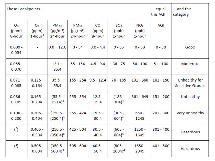
Our measures of air pollution are constructed from air quality data from the EPA. The Clean Air
Act requires every state to establish a network of air monitoring stations that take daily readings of
criteria pollutants, of which we consider fine particulate matter (PM2.5 ), particulate matter (PM10 ),
nitrogen dioxide (NO2 ), carbon monoxide (CO), and ozone (O3 ). For each pollutant, we construct
three county-month level measures: the average concentration, an air quality index, and the number
of poor air quality days. The air quality index is scaled from 0–500, and is based on methodology
from the EPA (see Section A.1.2). Poor air quality days are defined as days when the air quality
index exceeds 51.
There are three main caveats with these data. First, the number of air monitoring stations varies
the actual counts of registered vehicles in 2011. The process works very well—the correlation between the predicted
number of emissions-cheating diesels registered in 2011 and the actual number in 2011 is 0.992.
12across pollutants. Coverage is best for PM2.5 and ozone, with monitors in 556 and 731 counties in
2015, respectively, whereas fewer monitoring stations measure NO2 (monitors in 232 counties in
2015). Thus, we have qualified information about the direct effect of the cheating diesel cars on
NO2 , a component of NOx , which was the main pollutant excessively emitted by cheating diesel
cars. However, as mentioned above, NO2 is a primary precursor for PM2.5 and ozone (Hodan
and Barnard, 2004; Lin and Cheng, 2007). Lin and Cheng (2007) find that the majority of NO2
converts to particulate nitrate (a component of PM2.5 ) within a few days. Hence, increases in NOx
will directly translate into increases in PM2.5 and ozone, pollutants that are well monitored and
that are the most relevant for health impacts.18
Second, monitors and monitoring stations are added and discontinued frequently over the sam-
ple time. Furthermore, Grainger et al. (2016) provide evidence that regulatory agencies in compli-
ance with federal air quality standards strategically avoid pollution hotspots when choosing new
monitor locations. Systematic placement of new monitors in areas with less pollution could distort
the time trend of county-level pollution if we averaged across all available monitors in each period.
As a conservative approach, we use only one monitoring station per county to hold fixed the phys-
ical area where pollution is being measured over time. For each county and pollutant, we choose
the monitoring station with the most readings over our period and construct a county-month level
panel of pollution measures from 2007 to 2015. We show that results are very stable if we use
alternative measures based on several monitors per county.19
A third caveat is that even the longest-running monitor locations are not randomly assigned
within a county. Monitors are often located in or near cities (Muller et al., 2018), so that the sample
of counties with monitors tends to be more urban than the overall U.S. population. Moreover, if
regulators on average strategically place monitors away from pollution sources, and car pollution
18
PM2.5 and ozone are considered the most relevant in terms of health impacts of air pollution (for reviews, see
Hoek et al. (2013); World Health Organization (2013)), and are to a large extent caused by road transportation (Cames
and Helmers, 2013; Chossière et al., 2017).
19
We develop a procedure which averages across multiple monitoring stations at the county-month level, while
holding the geographical distribution of the monitoring stations fixed. In particular, we allow more than one monitor
per county (for example up to two monitors per county), but only use observations where all monitors report pollution
measures to avoid compositional changes from new monitors being added in different parts of the county.
13is very local, we could underestimate the effect of the cheating cars on pollution. However, the
high pollution levels of cheating diesel cars were not known to regulators, and over 85 percent
of the monitors we use predate the emissions cheating cars. Hence, it is unlikely that regulators
strategically placed monitors in order to avoid the pollution generated by cheating diesel cars.20
For PM2.5 , we can complement the monitor-based measure with an alternative which com-
bines satellite observations of aerosol optical depth, simulations from a chemical transport model,
and information from EPA monitors (van Donkelaar et al., 2019).21 There are advantages and
disadvantages to this alternative measure. On the positive side, the satellite-based measure offers
estimates of monthly PM2.5 for all counties in the US, rather than just the subsample with a PM2.5
monitoring station. On the negative side, satellite-based estimates are not direct measures, and
prediction errors appear both to be important and not well understood. In particular, Fowlie et al.
(2019) suggest that satellite estimates are biased down at high PM2.5 concentrations.
3.3 Birth data
Our first set of health outcomes comes from the U.S. National Vital Statistics System’s birth records
from 2007 to 2015. These data contain detailed information on all births in the United States,
including county and month of birth, demographic information about the mother, and health out-
comes for the infant, and are collapsed to the county-conception month. Conception month is cal-
culated by taking the gestational age in weeks and dividing by 4.345, rounding gestation months
to the nearest integer, and subtracting months of gestation from the birth month.
Our preferred measures of infant health are county-month average birth weight and the county-
month level fraction of babies born at low birth weight (less than 2500 grams). Birth weight is
often used as a summary measure of infant health, and low birth weight in particular is associated
with a range of poor outcomes, both health-related and economic, such as schooling and earnings
20
Relatedly, Zou (2018) shows that when pollution is measured intermittently (on six-day cycles), air quality is
worse on unmonitored days—suggesting strategic behavior over time as well as over the initial location of the monitor.
As the source of pollution is unknown in our context and the monitoring data aggregated to the monthly level, we do
not believe this type of high-frequency, strategic behavior will impact our analysis.
21
We are grateful to Wes Austin for providing us with cleaned county-month-level PM 2.5 satellite data.
14(Black et al., 2007; Almond et al., 2018). We further analyze county-month average gestational
age in weeks and the rate of premature birth (gestational age of less than 37 weeks). Birth weight
and gestational age are both commonly used summary measures of infant health.
3.4 Emergency department discharge data
Our second set of health outcomes comes from State Emergency Department Databases (SEDD)
from the Agency for Healthcare Research and Quality’s Healthcare Cost and Utilization Project
(HCUP), which contain the number of emergency department (ED) visits over time, by diagnosis,
from 2007 to 2015. We focus on the number of visits with a primary diagnosis of asthma, which
is known to be triggered by poor air quality and has been shown to be correlated with exposure to
traffic-borne pollutants (Gauderman et al., 2005).22 In particular, we construct the number of ED
visits for asthma per 1,000 people at the county-quarter level. We also break down this measure by
patient age, as young children are most likely to be affected.
Although the HCUP data are very detailed, there are two important caveats. First, the ED dis-
charge data do not include records for patients who were admitted through the ED. This limitation
means that the data are not well suited for analyzing more-severe health outcomes, such as strokes
or heart attacks, which typically result in a hospital admission. Second, we are limited by financial
considerations to a small subsample of states: Arizona, New Jersey, Kentucky, Rhode Island, and
Florida, providing us with 228 counties.
3.5 Other data
Our analysis further includes annual data on county characteristics from the U.S. Census Bureau’s
Small Area Income and Poverty Estimates program (SAIPE) and the Census Bureau’s Population
Estimates program (county-year level population, median income, fraction in poverty, fraction of
children in poverty, and fraction white), as well as the annual number of vehicle-miles driven by
state according to the Federal Highway Administration.
22
We use ICD-9 code 493 and ICD-10 code J45.
153.6 Cheating diesel over space and time
Figures 1A and 1B show the distribution of non-cheating diesel cars in 2007 and 2015. Non-
cheating diesel is strongly clustered in the western part of the United States, particularly in less-
populated rural states (these are mainly light-duty trucks). While there has been a slight increase
in the fraction of non-cheating diesel cars between 2007 and 2015, the spatial distribution is stable
over time. The pattern looks very different for the distribution of cheating diesel cars in Figures
1C and 1D. The 2007 map is blank as the first cheating diesel cars were not sold until 2008. By
2015, over 600,000 cheating diesel cars were sold (Figure A.1 shows annual registration counts),
clustered on the West Coast, the upper Midwest, and New England–areas that are typically thought
of as relatively wealthy and environmentally conscious. The distribution of “cheating” gas models
looks very similar to the cheating diesel map (see Figure A.2) indicating that diesel and gas model
were marketed to similar areas (they were also similarly priced; for details see Table A.14).
Figure 2 shows how the distribution of different car types is related to counties’ median income
in the 2015 cross-section. The left figure shows average median income across percentiles of
counties, ranked by their share of non-cheating diesel cars. Counties with high shares of non-
cheating diesel have somewhat lower median income than counties with fewer diesel cars (in line
with income gradients for overall air pollution (Muller et al., 2018)). The blue dots in the right
panel show that this relationship is reversed for cheating diesel cars. Counties with higher shares
of cheating diesel cars in 2015 have higher median incomes than those with lower shares. The
relationship is close to linear across the entire distribution, and it is strong: the median income in
the top percentile is almost twice as high as in the bottom percentile. The hollow green circles in
the right panel of Figure 2 show median income when counties are ranked instead by their share of
“cheating” gas models. T’he relationship is very similar to the cheating diesel gradient, suggesting
that areas in which people purchased many cheating diesel cars are similar to areas with many
“cheating” gas models. The same holds true for a broad set of maternal characteristics (Figures 7
and A.7).
163.7 Summary statistics
Table 1 shows summary statistics at the county-year-month level for the overall sample of counties,
for the sample of counties with a PM2.5 monitor, and for terciles ordered by the share of cheating
diesel in 2015.23 The upper panel shows counties’ car registration characteristics, demograph-
ics, and pollution outcomes. The lower panel shows birth outcomes and maternal characteristics,
restricted to county-year-month observations with non-zero births. We include observations with
zero births in the main pollution regressions in order to maximize the power of the analysis, though
results are unchanged if only county-year-months with non-zero births are used.
Comparing the first two columns, PM2.5 monitors are placed in counties that are more popu-
lated and that have slightly lower poverty rates and higher median incomes than the full sample of
counties. Birth outcomes and maternal characteristics are relatively similar between the full sam-
ple and the PM2.5 monitor sample. In line with Figure 2, median income increases across terciles
of the 2015 cheating diesel share. A higher cheating diesel share is also associated with a larger
population, a higher number of cars and miles driven, and lower poverty rates. Despite having
more cars, PM2.5 and PM10 levels are lower on average in counties with a higher cheating diesel
share. Mothers giving birth in counties with higher cheating diesel shares are more likely to be
white, married, more educated, and less likely to smoke during pregnancy. Not surprisingly, given
the positive selection of mothers, these counties have better average birth outcomes: higher birth
weight and longer gestation length.
4 Empirical strategy
We seek to estimate the effect of car pollution on health. Given well-measured experimental
23
Table A.1 shows summary statistics for the subsample of the five states for which we have HCUP data on emer-
gency department discharges. As in the overall sample, counties with higher shares of cheating diesel cars tend to have
higher median incomes and lower poverty. Asthma rates are hump-shaped, with the highest occurrence in the second
tercile and slightly lower rates in the bottom tercile than in the top tercile.
17variation in car pollution at the county-time level (Pct ), we would run the following regression
Healthct = α + βln (Pct ) + εct (1)
with β measuring the effect of a percent increase in car pollution on health. Running this
regression in available observational data likely results in a biased estimate due to endogeneity
and measurement error, and is nearly impossible to run due to lack of data on car pollution. As
discussed previously, we argue that the number of cheating diesel cars provides a well-measured
(conditionally) exogenous source of car pollution. Our preferred measure of exposure to cheating
diesel cars is the number of such cars per 1,000 cars in a county (cDct ).
How do changes in cDct relate to changes in total car pollution within a county? First, the
pollution stemming from one gasoline car (pi ) can be decomposed into miles driven times the
pollution per mile
pit = mit ∗ (poll/m)i (2)
Then, assuming that cars are either gasoline or cheating diesel cars, that all cars in a county drive
the same average miles mc , and that cheating diesel cars pollute as much as 100 gasoline cars per
mile (see Section 2.3), we can express a county’s total car pollution (Pct ) as:
cDct cDct
Pct = 1− ∗ pc ∗ Cct + 100 ∗ ∗ pc ∗ Cct
1000 1000
| {z } | {z }
pollution f rom gas cars pollution f rom cheating cars
(3)
99cDct
= 1+ ∗ pc ∗ Cct
1000
| {z }
total pollution f rom cars
with pc referring to the pollution stemming from a gasoline car driving mc miles and Cct referring
18to the total number of cars in a county.24 Thus, an increase of one cheating diesel car per 1,000
cars increases the total car pollution by about 10 percent for small baseline shares.25
δln (Pct ) 1
= ≈ 0.1 (4)
δcDct 9.9 + cDct
We also show results using alternative exposure measures, such as the number of cheating diesel
cars per 1,000 people or per square mile. However, these alternative measures do not relate as
directly to equation (1).
The strong spatial clustering of cheating cars described in the previous section implies that simply
comparing areas with higher and lower shares would not be informative. Our empirical strategy
therefore focuses on within-area comparisons over time. The fast roll-out of cheating diesel cars
into higher-income areas in combination with the deception of consumers regarding their actual
pollution levels provides us with identifying variation for a complier population of particular
interest. We will run several versions of the following regression:
Outcomect = α + β1 cDct + β2 cGct + λc + λt + δXct + εct (5)
where c indicates the county and t the time period (either monthly or annually). The dependent
variable Outcome refers to pollution, birth, or health outcomes (for birth outcomes t refers to the
conception month or year). The main regressor of interest is cD, referring to the number of
cheating diesel cars per 1,000 registered cars in a county. cG is the share of “cheating” gas cars
per 1,000 cars. λc and λt are county and time fixed effects and Xct are time-varying county
characteristics.26 The data are collapsed at the county-month level (we also show results using the
24
While we do not have data on miles driven by make of car, there is little relationship between average miles driven
per capita at the state level and share of cheating diesel cars, supporting the assumption that cheating diesel cars are
driven as similar amount as the average car.
25
Note that all counties start with a share of zero cheating cars and the median county has a share of only 1.6 per
1,000 cars in 2015.
26
Included characteristics are share of non-cheating diesel cars per 1,000 cars, log total cars, log population, poverty
rate, child poverty rate, and median income. Birth outcome regressions include additional controls for the following
19micro-level data and data collapsed to the county-year), and standard errors are clustered at the
county level. Observations in birth outcome regressions are weighted by the number of births.
When we focus on subgroups of mothers with various demographic characteristics, we use the
individual level micro data.
Finally, we present results from instrumental variable (IV) specifications in which we use the
cheating diesel share as instrument for PM2.5 and ozone. In regressions that include both PM2.5
and ozone, we interact the cheating diesel share with county-specific weather conditions (which
differently mediate the transformation of car exhaust into PM2.5 and ozone) to obtain additional
instruments (Knittel et al., 2016).
4.1 Identification
The inclusion of county and time fixed effects means that we compare changes in areas with in-
creasing cheating diesel shares (treatment counties) to overall time trends in the data. This is
essentially a difference-in-difference approach, with the identifying assumption that any trend de-
viations in the outcomes of treatment counties are driven by the changes in the cheating diesel
share. There is a common set of threats to this framework.
Increases in cheating diesel shares might be correlated with or driven by simultaneous socio-
economic changes that increase pollution and worsen health outcomes. A direct way to test for such
violation of the exclusion restriction is balancing regressions that use socio-economic indicators as
dependent variables on the left of the regression equation (Pei et al., 2018). We will show balancing
results both in binned scatter plots and in regression form.
Our estimates could also be confounded by selection due to unobserved characteristics, such
as tastes for new cars. We report the effects of counties’ “cheating” gas shares to explore the role
of such factors. As discussed above, the type of counties with high cheating diesel shares are very
similar in terms of socio-economic characteristics to counties with high “cheating” gas shares. If
maternal characteristics: fraction of mothers that are hispanic, black, married, smoking during pregnancy, average age,
and education bins.
20our results were driven by selection, we would expect to find similar effects of cheating diesel and
“cheating” gas cars on health outcomes.
While we think of the share of “cheating” gas cars as akin to a placebo conceptually, we are
only able to separately identify the effects of the two different types of cars because they have
slightly different patterns of dispersion. As we show in Figure A.3, both cheating diesel cars and
the equivalent gas models achieve higher market shares in counties with stronger preexisting de-
mand for these Volkswagen models. However, counties with both strong preexisting Volkswagen
demand and higher initial diesel shares accumulate somewhat more cheating diesel models relative
to “cheating” gas cars.27 Intuitively, the accumulation of both cheating diesel and “cheating” gas
cars are driven by brand preferences, while the difference between the two types is driven by pref-
erences for and availability of diesel fuel. Importantly, we will show that only cheating diesel cars
are associated with higher pollution and worse health outcomes, and this relationship is virtually
identical regardless of whether we also control for “cheating” gas cars.
Another potential concern are differential trends in treatment and control counties occurring
already before the treatment. Similarly, a spurious relationship in our setting could be caused
by strong outliers in single time periods. It would not be plausible if effects were driven by an
individual period despite the gradual dispersion of cheating diesel cars. We explore pretrends and
the role of individual years using an event study approach.
Finally, effects could be driven by changes in control areas, for example, if poorer counties with
few cheating diesel cars (“control counties”) experienced improvements in pollution and health
for reasons unrelated to diesel car penetration. Figure A.1 shows no evidence of a trend change
in pollution for such control counties. We also present robustness checks in which we exclude
counties with few cheating diesel cars.
27
Using data on diesel fuel availability in North Carolina, we can further show that both initial diesel shares and
ratios of cheating diesel to “cheating” gas models in a county are correlated with the fraction of gas stations with a
diesel pump (see Figure A.4).
215 Results
5.1 Effect of diesel emissions on pollution
We find large and statistically significant effects of the cheating diesel cars on air pollution. This
relationship is demonstrated semi-parametrically in Figure 3A, which shows binned scatter plots
of fine particulate matter air quality plotted against the fraction of cheating diesel, with county
fixed effects, time fixed effects, and vehicle composition variables partialled out. While there is
a strong relationship between the fraction of emissions cheating cars and PM2.5 , there is no such
relationship for “cheating” gas cars (3B shows analogous plots with the “cheating” gas share on
the y-axis).
The first panel of Table 2 reports effects on the air quality index (AQI) for the five analyzed
pollutants. We find strongly significant effects of cheating diesel cars on PM2.5 , PM10 , and ozone.
An additional cheating car per 1,000 increases the AQI for those three pollutants by 1.99 percent,
2.20 percent, and 1.33 percent, respectively. Effects on CO and NO2 are not significant at the 5
percent level. The second row shows the coefficients on the share of “cheating” gas cars. Point
estimates are small and imprecisely estimated but negative across all pollutants, which is what
one would expect given that these are newer models, and, absent the emissions cheating scandal,
newer models tend to be cleaner. The last line of each panel reports the p-value of a test of equality
between the cheating gas and cheating diesel coefficients; in nearly every case where the effect of
the cheating diesel cars on pollution is significant, we can also reject that the coefficients on the
diesel and gas versions are the same.28
The air quality index is particularly useful for comparing the magnitudes of the effects across
the pollutants, which have very different mean concentrations. Figure 4 plots the point estimates
in Table 2A, which helps summarize the results visually: there is a large effect of the fraction of
cheating diesel cars on air pollution, in particular on PM2.5 , PM10 , and ozone. Conversely, when a
larger share of the vehicle stock is made up of “cheating” gas cars, there is if anything slightly less
28
For brevity we do not show separate regressions including and excluding the control for “cheating” gas cars;
however, excluding this variable from the regression has no effect on the point estimate for cheating diesel cars.
22You can also read