Predicting Blood Glucose Levels of Diabetes Patients
←
→
Page content transcription
If your browser does not render page correctly, please read the page content below

Predicting Blood
Glucose Levels of
Diabetes Patients
Masterarbeit von Gizem Gülesir
Tag der Einreichung: 22. Januar 2018
1. Gutachter: Prof. Dr. Max Mühlhäuser
2. Gutachter: Sebastian Kauschke
Darmstadt, 22. Januar 2018

                                         Fachbereich Informatik
                                         Telekooperation
                                         Prof. Dr. Max Mühlhäuser
Erklärung zur Abschlussarbeit gemäß § 23 Abs. 7 APB der TU Darmstadt

Hiermit versichere ich, Gizem Gülesir, die vorliegende Masterarbeit ohne Hilfe Dritter und nur
mit den angegebenen Quellen und Hilfsmitteln angefertigt zu haben. Alle Stellen, die Quellen
entnommen wurden, sind als solche kenntlich gemacht worden. Diese Arbeit hat in gleicher
oder ähnlicher Form noch keiner Prüfungsbehörde vorgelegen.

Mir ist bekannt, dass im Falle eines Plagiats (§38 Abs.2 APB) ein Täuschungsversuch vorliegt,
der dazu führt, dass die Arbeit mit 5,0 bewertet und damit ein Prüfungsversuch verbraucht wird.
Abschlussarbeiten dürfen nur einmal wiederholt werden.

Bei der abgegebenen Thesis stimmen die schriftliche und die zur Archivierung eingereichte elek-
tronische Fassung überein.

Name: Gizem Gülesir           Datum:                   Unterschrift:

Thesis Statement pursuant to § 23 paragraph 7 of APB TU Darmstadt

I herewith formally declare that I, Gizem Gülesir, have written the submitted thesis indepen-
dently. I did not use any outside support except for the quoted literature and other sources
mentioned in the paper. I clearly marked and separately listed all of the literature and all of
the other sources which I employed when producing this academic work, either literally or in
content. This thesis has not been handed in or published before in the same or similar form.

I am aware, that in case of an attempt at deception based on plagiarism (S38 Abs. 2 APB),
the thesis would be graded with 5,0 and counted as one failed examination attempt. The thesis
may only be repeated once.

In the submitted thesis the written copies and the electronic version for archiving are identi-
cal in content.

Name: Gizem Gülesir           Date:                  Signature:
Abstract

Time series data is used for modelling, description, forecasting, and control in many fields from
engineering to statistics. Time series forecasting is one of the domains of time series analysis,
which requires regression. Along with the recent developments in deep learning techniques, the
advancement in the technologies personal health care devices are making it possible to apply
deep learning methods on the vast amounts of electronic health data. We aim to provide reliable
blood glucose level prediction for diabetes patients so that the negative effects of the disease
can be minimized. Currently, recurrent neural networks (RNNs), and in particular the long-short
term memory unit (LSTM), are the state-of-the-art in timeseries forecasting. Alternatively, in this
work we employ convolutional neural networks (CNNs) with multiple layers to predict future
blood glucose level of a diabetes type 2 patient. Besides our CNN model, we also investigate
whether our static insulin sensitivity calculation model’s results have a correlation with basal
rate of the patient. We use the static insulin sensitivity data with our prediction model, in
order to find out whether it contributes for a better prediction or not. Our experimental results
demonstrate that calculated static insulin sensitivity values do not have any correlation with
the basal rate. Our convolutional neural network model forecasts multivariate timeseries with
multiple outputs including the blood glucose level with a 1.0729 mean absolute error for the
prediction horizon of 15 minutes.

                                                                                                 2
Contents

1 Introduction                                                                                                                                     5
  1.1 Scope . . . . . . . . . . . . . . . . . . . . . . . . . . . . . . . . . . . . . . . . . . . . . . .                                         5
  1.2 Outline . . . . . . . . . . . . . . . . . . . . . . . . . . . . . . . . . . . . . . . . . . . . . .                                         6

2 Theoretical Background                                                                                                                           7
  2.1 Diabetes Mellitus . . . . . . . . . . . . . . . . . . . . .     .   .   .   .   .   .   .   .   .   .   .   .   .   .   .   .   .   .   .    7
  2.2 Basics of Machine Learning . . . . . . . . . . . . . . .        .   .   .   .   .   .   .   .   .   .   .   .   .   .   .   .   .   .   .    8
      2.2.1 Performance Measures . . . . . . . . . . . . .            .   .   .   .   .   .   .   .   .   .   .   .   .   .   .   .   .   .   .   10
      2.2.2 Types of Machine Learning Algorithms Tasks                .   .   .   .   .   .   .   .   .   .   .   .   .   .   .   .   .   .   .   12
      2.2.3 Learning Algorithm Types . . . . . . . . . . .            .   .   .   .   .   .   .   .   .   .   .   .   .   .   .   .   .   .   .   14
  2.3 Related Terms . . . . . . . . . . . . . . . . . . . . . . .     .   .   .   .   .   .   .   .   .   .   .   .   .   .   .   .   .   .   .   16
      2.3.1 Capacity, Overfitting and Underfitting . . . .            .   .   .   .   .   .   .   .   .   .   .   .   .   .   .   .   .   .   .   17
      2.3.2 Regularization . . . . . . . . . . . . . . . . . .        .   .   .   .   .   .   .   .   .   .   .   .   .   .   .   .   .   .   .   17
      2.3.3 Gradient Based Optimization . . . . . . . . .             .   .   .   .   .   .   .   .   .   .   .   .   .   .   .   .   .   .   .   18
  2.4 Artificial Neural Networks . . . . . . . . . . . . . . . .      .   .   .   .   .   .   .   .   .   .   .   .   .   .   .   .   .   .   .   19
      2.4.1 Deep Neural Networks . . . . . . . . . . . . .            .   .   .   .   .   .   .   .   .   .   .   .   .   .   .   .   .   .   .   20
      2.4.2 Optimization Algorithm Gradient Descent .                 .   .   .   .   .   .   .   .   .   .   .   .   .   .   .   .   .   .   .   21
      2.4.3 Backpropagation Algorithm . . . . . . . . . .             .   .   .   .   .   .   .   .   .   .   .   .   .   .   .   .   .   .   .   22
      2.4.4 Activation Function . . . . . . . . . . . . . . .         .   .   .   .   .   .   .   .   .   .   .   .   .   .   .   .   .   .   .   22
      2.4.5 Cost Function . . . . . . . . . . . . . . . . . . .       .   .   .   .   .   .   .   .   .   .   .   .   .   .   .   .   .   .   .   23
      2.4.6 Learning Rate . . . . . . . . . . . . . . . . . . .       .   .   .   .   .   .   .   .   .   .   .   .   .   .   .   .   .   .   .   23
  2.5 Deep Learning . . . . . . . . . . . . . . . . . . . . . . .     .   .   .   .   .   .   .   .   .   .   .   .   .   .   .   .   .   .   .   23
      2.5.1 Convolutional Neural Networks . . . . . . . .             .   .   .   .   .   .   .   .   .   .   .   .   .   .   .   .   .   .   .   23
      2.5.2 AutoEncoder . . . . . . . . . . . . . . . . . . .         .   .   .   .   .   .   .   .   .   .   .   .   .   .   .   .   .   .   .   26
      2.5.3 Long Short-Term Memory . . . . . . . . . . .              .   .   .   .   .   .   .   .   .   .   .   .   .   .   .   .   .   .   .   27

3 Related Work                                                                                                                                    29
  3.1 Blood Glucose Prediction Models . . . . . . . . . . . . . . . . . . . . . . .                                   .   .   .   .   .   .   .   29
      3.1.1 Physiological Models . . . . . . . . . . . . . . . . . . . . . . . . . .                                  .   .   .   .   .   .   .   29
      3.1.2 Data-Driven Models . . . . . . . . . . . . . . . . . . . . . . . . . . .                                  .   .   .   .   .   .   .   30
      3.1.3 Hybrid Models . . . . . . . . . . . . . . . . . . . . . . . . . . . . . .                                 .   .   .   .   .   .   .   31
  3.2 Insulin Sensitivity Assessment Models . . . . . . . . . . . . . . . . . . . .                                   .   .   .   .   .   .   .   31
      3.2.1 HOMA-IR (Homeostasis Model Assessment-Insulin Resistance)                                                 .   .   .   .   .   .   .   32
      3.2.2 QUICKI (Quantitative Insulin Sensitivity Check Index) . . . . . .                                         .   .   .   .   .   .   .   32
      3.2.3 FGIR (Fasting Glucose/Insulin Ratio) . . . . . . . . . . . . . . . .                                      .   .   .   .   .   .   .   32
      3.2.4 Glucose Clamp Technique . . . . . . . . . . . . . . . . . . . . . . .                                     .   .   .   .   .   .   .   32
  3.3 ANN Approaches . . . . . . . . . . . . . . . . . . . . . . . . . . . . . . . . .                                .   .   .   .   .   .   .   33

4 Data Resources                                                                                                                                  36

                                                                                                                                                   3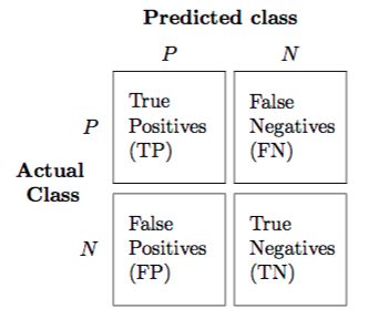
4.1 OpenDiabetesVault Framework . . . . . . . . . . . . . . . . . . . . . . . . . . . . . . . . 36
   4.2 Vault Database . . . . . . . . . . . . . . . . . . . . . . . . . . . . . . . . . . . . . . . . . . 36
   4.3 Static Insulin Sensitivity Calculation . . . . . . . . . . . . . . . . . . . . . . . . . . . . 38

5 Experiment Setup                                                                                                                                         40
   5.1 Preprocessing of Dataset . . . . . . . . . . . . . . . . . . . . . . . . . . . . . . . . . . . . 40

6 Experiments                                                                                                                                              42
   6.1 Convolutional Neural Network Model . . .            .   .   .   .   .   .   .   .   .   .   .   .   .   .   .   .   .   .   .   .   .   .   .   .   42
       6.1.1 Filter Length and Number of Filters           .   .   .   .   .   .   .   .   .   .   .   .   .   .   .   .   .   .   .   .   .   .   .   .   43
   6.2 Multivariate One-Step Prediction . . . . . .        .   .   .   .   .   .   .   .   .   .   .   .   .   .   .   .   .   .   .   .   .   .   .   .   44
   6.3 Multivariate Multiple-Step Prediction . . . .       .   .   .   .   .   .   .   .   .   .   .   .   .   .   .   .   .   .   .   .   .   .   .   .   45
   6.4 Evaluation of Models . . . . . . . . . . . . . .    .   .   .   .   .   .   .   .   .   .   .   .   .   .   .   .   .   .   .   .   .   .   .   .   48

7 Conclusion                                                                                                                                               51
   7.1 Summary . . . . . . . . . . . . . . . . . . . . . . . . . . . . . . . . . . . . . . . . . . . . . 51
   7.2 Future Work . . . . . . . . . . . . . . . . . . . . . . . . . . . . . . . . . . . . . . . . . . . 51

List of Figures                                                                                                                                            53

List of Tables                                                                                                                                             54

Bibliography                                                                                                                                               55

                                                                                                                                                            4
1 Introduction
Diabetes mellitus is a major and increasing global problem [38]. There are around 171 million
diabetes patients worldwide according to the study of [38]. This figure is predicted to rise to
336 million by 2030 [51], and it represents 4.4% of the world’s population. Short term com-
plications are hypoglycemia and hyperglycemia. The long term complications usually affect the
vascular system, central nervous system and organs such as kidneys and eyes. These long term
complications usually result in cardiovascular disease, retinopathy, and nephropathy. However,
the costly complications can be reduced by managing to keep the blood glucose level between
acceptable levels.
The control of the blood glucose level inside safe limits requires continuous monitoring of
blood glucose level. The most common method for type 1 diabetics is finger prick test which
is taken several times a day. These readings are used in order to adjust the required insulin
dose which keeps the blood glucose between certain levels. Besides the blood glucose measure-
ment, there are many other factors influencing the diabetes. Insulin type and dose, diet, stress,
exercise, illness, and pregnancy are some of the factors with significant influence on diabetes
theraphy. Continuous blood glucose meters (CGMs) and insulin pumps (IPs) provide ease of
measuring the blood glucose and better monitoring for the patient. Using the information pro-
vided by CGMs, patients can better adjust the injection of exogenous insulin. However, CGMs
require user interpretation. A system without the feedback system is called an "Open-loop sys-
tem". In open-loop systems insulin is delivered in a preprogrammed independent of the amount
of glucose measured. This type of glucose monitoring systems are common. Conversely, in
closed-loop systems, output of the system is used as a feedback loop. In such system, insulin or
other substances are given in response to a measured amount of glucose [42]. A system where
these devices can work in closed-loop fashion to maintain a steady blood glucose level with
minimal intervention from the patient, can be the next step in diabetes management. However,
according to [21] such systems are at research and development stage, but initial clinical trials
are promising.
1.1 Scope
The goal of this thesis can be roughly divided into two main categories. First of all, we want
to show whether our static insulin sensitivity calculation correlates with the basal rate or not.
Secondly, we want to predict future blood glucose levels of the diabetes patient. Additionally,
we want to find out whether this newly generated feature, the insulin sensitivity, can contribute
to the blood glucose level prediction when used as an additional feature. Therefore, type 1
diabetes is out of the scope of this thesis.
We will be discussing state-of-the-art methods for insulin sensitivity assessment and also our
method. Our insulin sensitivity assessment model is a minimal physiological model using few
parameters such as, continuous glucose measurement, and bolus insulin value. For blood glu-
cose prediction models we will briefly explain different model structures, also related work, but
in this thesis we use neural network approach which is a data-driven model. Even though, RNNs
and in particular the LSTM, are the state-of-the-art in timeseries forecasting, we use CNN. In-
stead of RNN, we use one-dimensional convolutional neural network model using a real dataset
5derived from a type 2 diabetes patient. The idea behind applying CNNs to time series forecast-
ing is to learn filters that represent certain repeating patterns in the time series and to use these
to forecast future blood glucose values. We belive that the layered structure of CNNs might
perform well on noisy time series as in the work of [6]. Since we use the insulin sensitivity
feature in our neural network model, the overall architecture of our model is considered as a
hybrid model.
1.2 Outline
This thesis is organized in following manner: Chapter 2 describes necessary information re-
quired for understanding the disease diabetes mellitus, basic machine learning principles and
related terms, artificial neural networks and deep learning. In chapter 3, state-of-the-art has
been covered. We also discuss their significance, contribution and downsides. In chapter 4, we
present structure of our dataset which is used in our experiments. In chapter 5, we introduce
frameworks and libraries used for the experiments. In the next chapter 6, we present our ap-
proach for calculation of static insulin sensitivity from the dataset and neural network model for
predicting the future blood glucose levels. Besides these, we also evaluate the results derived
from these models. In chapter 7 we conclude our work with a forward looking approach.
62 Theoretical Background
In this chapter we will explain; diabetes mellitus disease, why it occurs, how it can be treated
and the most important how we can contribute the treatment with our approach in this thesis.
In the following section, we discuss why machine learning algorithms are used, especially which
types of problems they are capable of solving. How a machine learning algorithm learns and
what are the metrics used to evaluate the performance of a machine learning algorithm. We will
explain also different types of problems where machine learning can be applied.
2.1 Diabetes Mellitus
Diabetes is a chronic disease due to a malfunction of the pancreas. Pancreas is an endocrine and
digestive organ that, in humans, lies in the upper left part of the abdomen. Besides the function
of helping the digestion, another function of the pancreas is to produce insulin hormone allow-
ing blood glucose absorption by the body cells. Hence, pancreas also responsible for regulating
the blood glucose. Insulin is a hormone released by the beta cells of the pancreas. The most
important glucose source is food items that are rich in carbohydrates.
Every cell of the body needs energy to function. Blood glucose can be absorbed by the body
cells, only with presence of insulin hormone, which is normally produced by pancreas. This hor-
mone with healthy people, produced just with a right amount, but with diabetes patients, addi-
tional insulin injections are needed. Figure 2.1 provides an overview how insulin and glucose
metabolism works. In the figure, the carbohydrates inside the food consumed by the patient,
provide glucose to the blood stream after it is digested and converted into a smallest building
blocks after digestion. Bread unit is used in for estimation of carbohydrate amount inside the
food consumed by the patient. One bread unit corresponds to approximately 10g − 12g of
carbohydrates.
Besides the normal blood glucose and insulin mechanism, there are two more important cases
to mention. Firstly, muscles need almost no insulin during the sport in order to make use of
the glucose. Secondly, the body has a protection mechanism to deliver quick energy for the
cases where blood glucose level is critically low or during a heavily stressed situation. Critical
level threshold is 50 mg/dl. Another source of glucose is the glucose store which can release or
backup glucose. When the dangerous situation is over, this mechanism works in the opposite
direction, retrieving glucose from blood to the glucose store. Another hormone called glycogen
controls this glucose release and backup. On the other side, working muscles are the other
factor consuming the glucose inside the blood. Since glucose absorption is only possible with an
insulin release, for the diabetes patients, an insulin pump which releases insulin into the blood
stream is needed. The insulin pump works with a sensor placed under the skin of the patient.
The sensor measures the blood glucose level periodically and provides these measurements to
the insulin pump. In this way the pump can calculate the required amount of insulin needed for
the patient and release it. The rate of insulin released from the pump is called basal rate of the
patient. Basal rate varies with each patient and can be programmed with the insulin pump. The
dose of insulin released according to basal rate called basal insulin which stabilizes the blood
glucose to an optimal value when the patient does not do any physical activity and does not eat
anything.
7Figure 2.1: Illustration of insulin-glucose system
Disease arises from the reason; either the pancreas cannot produce enough insulin, or the
body cannot effectively use the produced insulin. When diabetes is not responded with a suitable
treatment, it leads to serious damage to the body’s systems. When the blood glucose level
is higher than the normal value, it is called hyperglycaemia, conversely low blood glucose is
named hypoglycaemia. In the next paragraph, we will discuss two types of diabetes and other
related effects in more details.
Type 1 diabetes patients characterized by deficient insulin production, while type 2 diabetes
patients by ineffective use of insulin. Majority of the diabetes patients are type 2. In the scope
of this thesis, we will be focusing on type 2 diabetes hypoglycemia prediction and prevention
using machine learning techniques. For type 2 diabetes patients, controlling the blood glucose,
and improving the insulin sensitivity is possible by changing life style and healthy diet. In order
to keep the blood glucose within normal level, diabetic person needs to inject certain amount
of insulin into the tissue between body skin, and the muscle. If the insulin is not injected, it
also could be inhaled with an inhaler or it can be infused with a pump. Insulin amount needed
is calculated based on food intake which is considered in terms of bread units. Blood glucose
level is highly dependent on injected insulin amount and food intake. Besides food intake, other
factors such as exercise, sleep-wake cycles, sleep quality, stress, illness, alcohol are known to be
affecting blood glucose mechanism. We summarize the other known effects which are known
to be influencing the blood glucose values, in the table 2.1.
2.2 Basics of Machine Learning
A machine learning algorithm which is able to learn from data [17] is used to tackle with
tasks, which are too difficult to solve with ordinary programs designed and written by human
beings. Machine learning algorithm processes collection of features measured from an object
or event. In order to simplify things, we will refer to an experience as E, class of tasks as T ,
and a performance measure as P. In the context of machine learning tasks, T are, tasks which
8Known Effects Description
Refill Effect After longer periods (>30 min) of sports, a blood glucose degra-
dation can be observed up to 10 hours after the event. This is
caused by a refill of the glucose stores of the body, since the stored
glucose is used to provide enough energy for the working muscles.
Dawn Phenomenon It is an early morning (usually between 2 a.m. and 8 a.m.) in-
crease in blood glucose. It is not associated with nocturnal hypo-
glycemia (low blood glucose value). The dawn phenomenon can
be managed by adjusting the dosage of the basal insulin in the
insulin pump.
Chronic Somogyi Rebound Chronic Somogyi Rebound describes a very high blood glucose
value after a hypoglycemia (low blood glucose value). It occurs
almost every time when the blood glucose value falls below 50
mg/dl (sometimes even earlier). The high blood glucose value is
caused by a panic release of the glucose reserves in the body. This
is triggered by hormone like Glucagon, Adrenalin and Cortisol.
Temporal Insulin Resistance After longer periods without eating carbohydrates, a temporal in-
sulin resistance can occur. However, patients have to inject more
insulin to overcome this effect. But mostly patients do not notice
this effect, and just wonder why the insulin dose does not work.
In order to prevent this effect, the patient should consume small
amounts of carbohydrates on a regular basis (3 times a day is
suggested).
Table 2.1: Known Effects of Diabetes Mellitus
9are too difficult to solve with fixed programs or human beings. When a computer program is
learning from experience E with respect to some class of tasks T , and performance measure P;
its performance at tasks in T , as measured by P, is called improving with the experience E [26].
Most of the machine learning algorithms can be thought as experiencing the entire dataset
during the training phase, in supervised or unsupervised manner. A dataset can be considered
as a collection of many examples or data points. In most of the cases, a dataset is a collection of
examples, which turns into a collection features by the training. For example; a design matrix
can be used to describe a dataset, which contains a collection of different example within every
row. In other words, we can represent a dataset with 150 examples, and with 4 features for
each example as X ∈ R1 50x4, where X i,1 corresponds to the first feature, X i,2 is the second
feature, and so on. Another way of expressing a design matrix is, defining each example as a
vector, each with the same size. However, this is not always possible, especially when the dataset
is heterogeneous. For example; a dataset consisting of photographs with different dimensions
(width and height) would result into images with different size and number of pixels. Therefore,
with the vector representation, it is not possible to represent all the examples. In some cases
with the heterogeneous data, instead of using a matrix with m rows to describe a matrix, it is
possible to use the representation {x (1) , x (2) , ..., x (m) } which corresponds to a set containing m
elements. With this notation, there might any two example vectors x (i) and x ( j) different sizes
in the dataset exist.
Depending on the dataset, the learning can be categorized as supervised and unsupervised,
even though the line between them is not sharp. The other variant of learning algorithm also
called semi-supervised learning, which involves some supervision to the unsupervised learning.
Machine learning can be used for solving many tasks. We will mention some of these tasks,
such as; classification, regression, anomaly detection, and denoising. However, the list can
be expanded. In order to accomplish the learning, the desired features from the dataset, cost
function, and optimization algorithm are required. Another basic requirement for the machine
learning is the performance evaluation, a measure how well the learning has done. In the
next section we will be describing these different performance evaluation metrics, and different
machine learning tasks and algorithms types.
2.2.1 Performance Measures
In order to evaluate the abilities of a machine learning algorithm, a quantitative measure is
needed. This quantitative measure P, is specific to the task T , which is carried out by the
learning algorithm. Performance metrics are used for defining, how well the machine algorithm
is performing the tasks. Decision process of performance metric is a difficult task, and should
be considered closely with the requirements of the application. For different machine learning
task categories, there are different metrics with different granularity used for measuring the
performance of the model. For example, for a regression task, error rate corresponds well to
the desired behavior, on the other hand, accuracy metric is well suited for a classification task.
For some problems penalizing the frequent medium sized mistakes, conversely for some others,
penalizing rare but large mistakes might fit. During a machine learning algorithm is training
using the data points, it is experiencing the training dataset. Evaluation of the learning should
be done with a separate test dataset, which is not seen during the training phase. Next section
we will be discussing about these different types of machine learning algorithms.
10Figure 2.2: Confusion Matrix Layout for Error Visualization
Classification Metrics
One of the performance metrics used for the tasks of classification is accuracy. It is calculated
from the proportion of examples, the model gives the correct output to all outputs. Error rate
is also used for measuring the accuracy of a machine learning model, where the proportion
of examples giving the incorrect output are used for the measurement. In order to introduce
the formula of accuracy, we introduce the concepts of sensitivity and specificity which are also
known as true positive rate and true negative rate.
A classifier classifies the outcome into positive and negative, as in the table 2.2 1 . When
the classifier predicts positive and the actual value is also positive or negative, this is called
True Positives (TP) and False Positive (FP) respectively. Similarly, when the classifier predicts
negative and the actual value is also positive or negative, this is called False Negative (FN),
and True Negative (TN) respectively. Accuracy is simply the fraction of the total sample that is
correctly identified. In other words, accuracy is the ratio of training examples which produces
correct output to the total number of training examples. Therefore, accuracy can be formulated
using these terms as follows:
TP + TN
Accur ac y =
TP + TN + FP + FN
For the tasks of classification, and classification with missing inputs, accuracy is the metric
used to measure the performance of the model. Error rate is another metric also used to derive
the same information, other way around. Error rate is the ratio of training examples which
produces wrong output to the total number of training examples. It is also referred as the
expected 0-1 loss. The 0-1 loss on particular example is 0 if it is correctly classified, and 1 if it
is not correctly classified. For some tasks, such as density estimation, none of the performance
1
Adapted from https://rasbt.github.io/mlxtend/user_guide/evaluate/confusion_matrix/
11metrics we discussed till now, is suitable. For such tasks, a performance metric which gives a
continuous-valued score for each given example should be used. Usually, in order to report the
average log-probability, the model itself assigns to some examples.
Regression Metrics
One of the popular metrics for measuring the performance of a regression model, is mean
absolute error (MAE). It is also called quadratic loss function. It is widely used in regression
tasks as a performance measure. It is expressed with the following formula:
n
1 X (i)
M AE = ŷ − y (i)
n i=1
where ŷ is the predicted value and y is the original value. The parameter n represents number
of data examples. Therefore, it is an average of the absolute errors the prediction and the true
value.
Second important metric is Mean Squared Error (MSE), which is also similar to MAE. MSE
is always positive value, since it takes the square of the difference between the prediction and
the real value. Therefore, it provides the gross idea of the magnitude error, and represented as
follows:
n
1 X (i)
M SE = ( ŷ − y (i) )2 .
n i=1
Another variation of this metric is called Root Mean Squared Error (RMSE), as its name sug-
gests; it takes the square root of MSE. Since this metric takes the square root of MSE, it converts
back the unit into its original units of the output variable. Therefore, it provides more meaning-
ful representation. This metric is described with the following formula:
v
n
t1
u X
RM SE = ( ŷ (i) − y (i) )2 .
n i=1
2.2.2 Types of Machine Learning Algorithms Tasks
In this section we describe different machine learning tasks.
Classification
This type of task, computer program is expected to categorize the input into one of the available
categories. The computer program is asked to solve the problem by producing the function
f : Rn → {1, ..., k} where k is the number of possible class labels. When y = f (x), the learned
model is able to assign the input vector x into the correct category k, identified by numeric code
y. In other words, learning algorithm must learn a function, which maps the input vector to a
12categorical output. Computer program, which can recognize handwritten digits and numbers,
is one of the application examples.
More difficult variant of classification is the classification with missing inputs. In this case,
computer program might get an input vector with missing measurements. A computer program
has to use a learning algorithm, which can learn a set of functions, rather than only a single
function. Each function corresponds to classifying x with a different subset, where some of
its input is missing. In case of this type of classification problem with n inputs, 2n different
classification functions needed for each set of possible missing inputs, but computer program
only has to learn a single function which describes the joint probability distribution.
Regression
In this type of task computer program is expected to predict a numerical value, rather than a
class label. A computer program predicting the future number of passengers’ based on previous
years of passengers’ data is a regression problem. Learning algorithm is asked to output a
function f : Rn → R, similar to classification task, except the format of the output. Similarly, it
can be also used to find similarities between two variables. One of the basic regression problems
is a linear regression. The goal of the algorithm is to predict a scalar value from the given input
vector. Linear regression models’ performance can be measured in terms of the squared error
produced when test data set given as an input.
Anomaly Detection
In this type of task computer program is expected to point out unusual events or objects from a
set. These unusual events do not conform to the expected behavior, and usually referred to as
anomalies, outliers, discordant observations, exceptions, aberrations, surprises, peculiarities or
contaminants in different application domains [7]. One way is, training the machine learning
model to be able to reconstruct the original input with minimum error rate. After the model is
trained, anomalous input will cause a higher error rate than the usual non-anomalous examples.
Anomaly detection has an extensive use in many applications such as fraud detection for credit
cards, intrusion detection for cybersecurity domain, fault detection for safety critical systems
and military surveillance for enemy activities.
Similar to anomaly detection, novelty detection aims to detect previously unobserved, emer-
gent or novel patterns in the data. The distinction between novel patterns and anomalies, is
that the novel patterns are typically incorporated into the normal model after being detected.
The solutions for mentioned problems are used often for both anomaly and novelty detection
problems.
Denoising
In this type of task, computer program is expected to recover the clean example x ∈ Rn from its
corrupted version x̃ ∈ Rn . This task is similar to anomaly detection, except instead of training
the model with original data, slightly corrupted version of it if given as input. Learning algorithm
learns to derive clean example x from its corrupted version x̃, while predicting the conditional
probability distribution p(x|x̃). Error rate is calculated based on the difference between the
13Cluster Genres Included
Short, Drama, Comedy,
Cluster 1 Romance, Family, Music,
Fantasy, Sport, Musical
Thriller, Horror, Action,
Cluster 2 Crime, Adventure, Sci-Fi,
Mystery, Animation, Western
Documentary, History,
Cluster 3
Biography, War, News
Reality-TV, Game Show,
Cluster 4
Talk Show
Cluster 5 Adult
Table 2.2: Outcome of movie clustering , adapted from [43]
produced output, and original version of the input. Therefore, the model is forced to learn the
noise and corrupted parts, during the training process [32].
2.2.3 Learning Algorithm Types
In this section, we explain different types of learning algorithms, and the main differences
between them. Machine learning algorithms can be roughly divided into 4 categories; unsuper-
vised, supervised, semi-supervised and reinforcement learning algorithms.
Unsupervised Learning
When the algorithm experiences and learns useful features and structure of a dataset; the algo-
rithm is called an unsupervised learning algorithm. Unsupervised learning is used for density
estimation, synthesizing, denoising and clustering. There is no instructor or teacher, who shows
the machine learning system what to do. The algorithm should find out a way to extract useful
properties of the given dataset. In the context of deep unsupervised learning, the entire prob-
ability distribution of the dataset is aimed for tasks such as density estimation, synthesis, and
denoising. Unsupervised learning algorithms observe several examples of random vector x, and
tries to learn the probability distribution p(x), or some other interesting properties of the dis-
tribution. There are other unsupervised learning algorithms doing clustering, which is dividing
the dataset into many similar examples. For example; clustering movies into different subsets,
based on their titles and keywords, using the similarity is one of the applications of clustering.
With or without providing the possible outcomes, the possible genres, the algorithm produces
different clusters. The table 2.2 has the outcome of movie clustering which carried out in the
work of [43].
Supervised Learning
When a machine learning algorithm experiences a dataset, and each example of the dataset has
an associated label, the algorithm is called a supervised learning algorithm. Training process
14involves observation of several labelled examples acting as a teacher, and showing the algorithm
how to learn the target from the given dataset. Label could be a number or a sequence of words.
For example, of speech recognition scenario, record of speech would have a sequence of words
as a label. Some of the supervised machine learning algorithms are logistic regression, support
vector machine (SVM), k-Nearest Neighbors, Naive Bayes, random forest, and linear regression.
For supervised learning, an example contains a label or target and collection of features.
Labels can be represented with a numeric code or sequence of words depending on the task.
When the dataset contains a design matrix of feature observations X , we also provide a vector
of labels y, with yi providing the label for an example i.
Unlike unsupervised learning algorithm, supervised learning algorithm involves observation
of several examples of input vector x, and associated output vector y and given together of
this information, algorithm tries to predict y from x during the training usually by estimating
p( y|x). Even though there is no instructor or teacher for unsupervised learning, sometimes the
line between supervised and unsupervised learning is blurred [17]. Usually these techniques are
categorized as semi-supervised learning[54]. We discuss semi-supervised learning in the next
section.
Even though supervised and unsupervised learning algorithms are not completely distinct
concepts, helps us to categorize the learning algorithms. For example; usually regression, classi-
fication, and structure output problems are considered as supervised learning algorithm, while
density estimation in support of other tasks is considered as unsupervised learning algorithm
according to [17].
Semi-supervised Learning
Another variant of machine learning algorithm including both supervised learning practices by
a supervision target and unsupervised fashion, is called semi-supervised learning algorithm.
For example; in multi-instance learning algorithm, an entire collection of input examples are
labeled as containing or not containing an example of a class, but the individual members of the
collection are not labeled.
Majority of the data in real world is unlabeled, and the process of labeling is time consuming
task. Therefore, these techniques can use the advantage of both labeled and unlabeled data.
There are many machine learning techniques can be used for both of the learning tasks. As
an example; an image classifier which uses both supervised and unsupervised methods can be
considered [18]. Another example, in the work of [18] a strong Multiple Kernel Learning (MKL)
classifier using both the image content and keywords is used in order to score unlabeled images.
Afterwards, the techniques; support vector machines (SVM) or least-squares regression (LSR)
from the MKL output values on both the labeled and unlabeled images are used.
Reinforcement Learning
Unlike the previous machine learning algorithms, reinforcement learning interacts with the en-
vironment during the learning process, besides experiencing the dataset. Interaction with the
environment happens within a feedback loop between the experiences and the learning system.
Reinforcement learning algorithm does not experience a fixed dataset like other supervised and
unsupervised learning algorithms. Popular applications of reinforcement learning are used with
15computer programs learning to play games such as chess, Go, Atari [28] and [27]. In this thesis
reinforcement learning methods are not used.
2.3 Related Terms
In this chapter, we use the one of the simple machine learning algorithms, in order to ex-
plain some related terms of machine learning algorithms. After quick introduction to machine
learning algorithm; the linear regression, we explain the terms overfitting, underfitting, regu-
larization, gradient based optimization. As the name suggests, linear regression is a machine
learning algorithm, which is used for solving regression problems with a linear function. The
algorithm takes a vector x ∈ R as an input, and tries to predict the value of scalar y ∈ R as an
output. The function of linear regression can be written as:
ŷ = w T x,
where w ∈ Rn is a vector of parameters, and ŷ is the prediction and the value y is the actual
value. The parameters w and x control the behavior of the system. In this equation, w i is the
coefficient that is multiplied by the feature x i , and the result is summed up together with all
the contributions from all feature vectors. If a feature received positive value from the weight
vector w i , the contribution of the feature vector x i increases on the prediction value ŷ. When
the weight value is negative, the effect of that specific feature decreases on the prediction. De-
pending on the magnitude value of the weight value, prediction changes. Therefore, if feature’s
weight is zero, it has no effect on the prediction. For linear regression the task, T is to predict y
from x by outputting ŷ = w T x.
For the performance measure P, there is a need for a test dataset, which is not used for the
training. One way is by computing the mean squared error of the model on the test set. Assum-
ing a model with a design matrix of m example inputs, the inputs of the design represented as
X (t est) , and the vector of regression target represented as y (t est) . The prediction ŷ (t est) can be
evaluated with the performance measure P as follows:
1 X (t est)
M SE t est = ( ŷ − y (t est) )2i .
m i
The error decreases when the difference between the prediction ŷ (t est) , and the target y (t est)
getting closer to the zero. Similarly, another performance metric can be defined in terms of
Euclidean distance between the prediction and the target as follows:
1
M SE t est = || ŷ (t est) − y (t est) ||22 .
m
In the equation above the total error decreases when the Euclidean distance between the
prediction and the target increases. Therefore, in order to a machine learning algorithm to
function correctly, it should either decrease the mean squared error, or increase the Euclidean
distance between the prediction and the target, while it is experiencing the training dataset.
To achieve minimization of the mean squared error on the training set M SE t r ain , the algorithm
should adapt its weights w accordingly.
16Linear regression often used to refer to slightly different model with an additional parameter
which is usually called bias b, which makes the new equation:
ŷ = w T x + b.
The additional parameter b makes the plot of the model still linear, but instead just not passing
through the origin. The terminology of the word bias is different from the statistical point of
view. It can be thought as the output is biased towards, based on the value of the parameter b.
Linear regression is one of the simplest machine learning algorithms. Therefore, it has limited
use for different problem types. In the following sections we will be discussing more sophisti-
cated algorithms and more terms related with machine learning.
2.3.1 Capacity, Overfitting and Underfitting
The ability of a machine learning model performing well on unseen data (test dataset) is called
generalization ability of the algorithm. During the training of the model, training error is used
as a performance in order to reduce the error rate on the training set. For example, measuring
the performance of the test phase of a machine learning algorithm, we have to have certain
assumptions about the train and test dataset. First of all, training and test sets should be in-
dependent from each other. Another assumption is; both sets should be identically distributed.
In other words, both sets should be drawn from the same probability distribution. When these
assumptions hold, training error of randomly selected model should be equal to the expected
test error of that model, since both are formed from the same data sampling process.
All machine learning algorithms aims to reduce the training error, and the difference between
the training and test error. While trying to achieve these goals, the main challenge is to be able
to fight with underfitting and overfitting. Capacity of a neural network is one of the important
factors of over and under fitting. Capacity of a neural network is directly related with the size of
the network. A neural network with more hidden layers and more hidden nodes tend to store
more information, therefore they have more capacity according to [49]. When the model has
high capacity, it starts to memorize the properties of the training test, instead of learning. This
happens when model has high generalization error, also called testing error. An overfitted model
performs poorly on unseen test data, while performing well on training data. In this case, the
model’s capacity is reduced in order to avoid overfitting. On the other hand, when a model has
low capacity, it is likely to underfit, which means it can not derive the essential features from the
training set. Underfitting takes place when the gap between training and generalization error is
too large, which is illustrated in the figure 2.3 in the area after the optimal capacity.
As a summary, machine learning algorithm has the best performance with the right capacity,
and also requires less amount of time for the training. Machine learning models with insufficient
capacity, fail to solve complex tasks, similarly models with high capacity fails to generalize well
and overfit for the tasks.
2.3.2 Regularization
Another method used to control overfitting and underfitting is regularization. It is any modifica-
tion made to a learning algorithm, in order to reduce its generalization error while not changing
the training error [17]. One way to do this for the linear regression algorithm, is modifying the
17Figure 2.3: Illustration of Overfitting and Underfitting, adapted from [17]
training criterion to include weight decay. Regularization adds a penalty on the different param-
eters of the model. Therefore freedom of the model is reduced by adding the penalty. As a result
of this, the model will be less likely to fit the noise of the training. Therefore regularization im-
proves the generalization abilities of the model. However too much regularization increases the
testing error rate, and leaving the model with too few parameters, which would not be able to
learn the complex representations from the input.
There are three types of regularization methods; namely L1, L2 and L1/L2. In L1 regulariza-
tion some of the model parameters are set to zero. Therefore those parameters no longer play
any role in the model. L2 regularization adds a penalty equal to the sum of the squared value of
the coefficients. Therefore, L2 regularization will force the bigger parameters for bigger the pe-
nalization, while on the smaller coefficients effect penalty is smaller too. For any other machine
learning algorithm, there are many ways to design regularization technique. Therefore, there
is no regularization form which fits to all of the machine learning algorithms. Regularization is
one of the central concerns of the field of machine learning, such as optimization problem.
2.3.3 Gradient Based Optimization
Optimization is a task of minimizing or maximizing a function f (x) by altering x. The function
f (x) is called objective function or criterion. For the maximization of f (x) is also referred as cost
function, loss function, or error function. We will use the notation x ∗ to refer the ar g min f (x).
The derivative function is used for minimizing, since it provides the information how to
change the x in order to minimize for the function y = f (x) at the point x. The derivative
dy
of a function f (x) is denoted as f 0( x) or d x . The figure 2.6 at page 21 provides visual. This
derivative function provides the direction information, from the red region where the cost is
high, towards which direction to move in order to reach the blue region(where error is mini-
mum). We will discuss gradient based optimization in more details in the section 2.4.2.
18Figure 2.4: Artificial Neuron Model
2.4 Artificial Neural Networks
Artificial Neural Networks (ANNs) are computational model which is inspired from biological
neurons of human brain [10]. The figure 2.5 2 on page 20 has typical ANN structure with input,
hidden and output layer. ANNs are called networks, because they are typically represented by
composing together many functions. A neural network with 3 layers can be considered as com-
puting the formula f (x) = f (3) ( f (2) ( f (1) (x))). First layer is f (1) , second layer is f (2) , and third
layer is f (3) of the neural network. ANNs are invented to solve tasks specifically humans are
good at, such as pattern recognition and other tasks which does not require to be re-programmed
and the tasks involving uncertainty. Therefore, ANNs have potential of solving many real life
problems in a wide range of fields. They contain layers of computing nodes called the percep-
tron doing the nonlinear summation operation. A neuron fires when a particular function of
summation of the signals outcome is greater than some threshold value.P The neuron in fig-
ure 2.43 with three incoming connections and the activation function of i (w i x i + b). Nodes
within each layer are interconnected by weighted connections, where weights are represented
with w i . Signal strength depends on the weighted connections. Therefore, while some neurons
are passing the signal to the next layer, some might drop. ANNs have an input and output lay-
ers. The middle layer is known as hidden layer. ANN having at least one hidden layer is capable
of solving nonlinear tasks by training with gradient descent methods. ANNs with many hidden
layers are called deep neural networks.
Before neural network is trained, its weights are usually initialized by a random distribution
function. At this stage ANN is not expected to produce any meaningful result. Input data is
fed during the training phase. By the time, over iterations, weights of the neural network are
adjusted in order to output according to the desired function. In other words, neural network
changes its weights, in order to adapt new environment requirements during its training [13].
During the supervised learning of a neural network, both the input and the correct answer
is provided. The input data is propagated forward from input layer to the output neurons.
Outcome of propagation is compared with the correct answer. Based on the difference between
outcome and the correct answer, weights of the network are adjusted in a way to increase the
probability of the network giving correct answer for the future runs with the same or similar
2
Adapted from http://cs231n.github.io/neural-networks-1/
3
Adapted from https://towardsdatascience.com/from-fiction-to-reality-a-beginners-guide-to-artificial-
19Figure 2.5: Artificial Neural Network Structure
data. For unsupervised learning, no correct answer, but only input data is provided. Network
has to evolve by itself according to some structure, which in the given input data. Usually
the structure is a some of form redundancy or clusters in the given input data[13]. Another
important property of neural network training, as well as all machine learning algorithms is,
how well the network generalize after the training. In the case of overlearning set of training
input data is called overfitting. Since the network does not generalize well, it performs poorly
with the unseen test data. While the number of hidden neurons provides a degree of freedom,
on the other hand increases the risk of overfitting, because the network will tend to memorize
the data. In order to overcome this problem some weights removed explicitly to increase the
generalizability of the neural network. In case of too few hidden layer neurons, network might
not perform the desired functionality. Therefore, a compromise should be found while designing
neural network.
In the next sections we will be discussing the different types of neural networks and related
terms.
2.4.1 Deep Neural Networks
Feedforward neural networks with more than one hidden layers are called deep neural networks
or deep-learning networks. Deep neural networks are used to approximate some function f ∗.
For classification task, y = f ∗ (x) maps an input x to a category y. The neural network defines
a mapping y = f (x; θ ), and learns the value of the parameters θ which would result in the best
possible approximation. In deep-learning networks, each layer of nodes trains on a distinct set of
features based on the previous layer output. The further hidden layer added to the network, the
more complex the features can be recognized, since they aggregate and recombine features from
the previous layer. Besides this, training becomes also harder and takes longer time compared
to shallow neural networks and perceptrons.
The reason why these neural networks are called feedforward, is the information flows from
the input layer direction towards the output layer through the intermediate computations. The
20Figure 2.6: Gradient Descent Algorithm Illustration
simplest form of learning algorithm with feedforward neural is called perceptron, input and out-
put layers do not learn the representation of the data, because they are predetermined unlike
the hidden units. When feedforward connections have feedback connections, they are called
recurrent neural networks. Another type of specialized feedforward neural network is convolu-
tional neural networks, which specifically used for object recognition tasks. We describe some
of these deep neural network types in the further sections.
2.4.2 Optimization Algorithm Gradient Descent
Learning of deep neural networks requires gradient computation of many complex functions,
similar to any other machine learning algorithm. Besides the gradient algorithm, one needs to
specify an optimization procedure, a cost function and a neural network model. The algorithm
tries to find the best parameters for network with minimum cost. The figure 2.64 represents
the cost space. The areas with red color has the highest cost, while blue regions has the lowest
cost. The optimization algorithm tries to find the path down from the point of the highest cost
to the regions where the cost is lowest. Therefore, y-axis, we have the cost J(θ ) against the
parameters θ 0 and θ 1 on x-axis and z-axis respectively. However there are certain challenges
with optimization of the algorithms, such as vanishing or exploding gradient problem. Some-
times gradient signal is too small. Therefore, algorithm cannot converge to the global optima.
Similarly, when gradient signal is too strong, and bigger steps are taken, again algorithm cannot
converge. Since it keeps bouncing around the curvature of the cost valley, overshooting the
correct path. It is not always straightforward to find the global optima. Hence, there are many
variations of gradient descent algorithm. Some other variations are vanilla gradient descent,
gradient descent with momentum, AdaGrad (Adaptive Stochastic (Sub)Gradient) and ADAM
(Adaptive Momentum).
Gradient descent algorithms can be roughly classified as two methods; full batch gradient
descent algorithm, and stochastic gradient descent algorithm. Full batch gradient descent algo-
rithm the parameters are updated after the use of the full batch of the input data, while with
the stochastic gradient descent algorithm, the parameters are updated only after whole dataset
is used. We discuss one of gradient algorithm, which is back-propagation algorithm, and its
modern generalizations in the next section.
4
Adapted from http://cs231n.github.io/neural-networks-3/#sgd
212.4.3 Backpropagation Algorithm
Backpropagation is learning procedure for networks neurone-like units [39]. The backprop-
agation algorithm repeatedly adjusts the weights of the connections based on the difference
between the actual output vector, and the desired output vector. The algorithm uses the partial
derivative of the error of the neural network with respect to each weight [1], in order to min-
imize the difference between two vectors. The process of modification of each weight, starts
from output layer and last hidden layer connection, and propagates through each layer until it
reaches the input layer. Therefore, it is called backpropagation algorithm. Using these partial
derivatives, and the change of the value of the weight, networks weights are adjusted to reach
the local minimal. In other words, if the derivative is positive the error is increasing. When the
weight is increasing, then backpropagation algorithm adds a negative value of partial derivative
to the weight in order to minimize the error. Similarly, if the derivative is negative, then it is
directly added to the weight. The basic idea of the backpropagation learning algorithm is the
repeated application of the chain rule to compute the influence of each weight in the network
with respect to an arbitrary error function E [37] as follows:
∂E ∂ E ∂ si ∂ net i
=
∂ wi j ∂ si ∂ net i ∂ w i j
where w i j is the weight from the neuron j to neuron i, si is the output, and net i is the weighted
sum of the inputs of the neuron i. Once the partial derivatives for each weight is known, the
aim of the minimizing the error function is achieved by performing a simple gradient descent:
∂E
w i j (t + 1) = w i j (t) − ε (t)
∂ wi j
The choice of learning rate ε, scales the derivative and effects the time needed until convergence
is reached. If the learning rate is too small, too many steps are needed to reach an acceptable
solution. On the other hand, too big value possibly leads to oscillation, preventing the error to
fall below a certain threshold value. In order to cope with this problem another variable called
momentum parameter is added. However setting the optimum value of momentum parameter
is equally hard as finding the optimal learning rate value.
2.4.4 Activation Function
Feedforward networks have introduced the concept of a hidden layer, therefore activation func-
tion is needed in order to compute hidden layer values. In simple words, activation function
calculates the sum of weighted inputs from the previous layer of the network, adds the bias
value of the neuron to it, and then decides whether the neuron should be fired or not. The
most popular activation functions are logistic function 1+e1−x , t anh() function, and The Rectified
Linear Unit (ReLU) function f (x) = max(0, x). The ReLU makes the network converge faster,
and it is resilient to the saturation. Therefore, unlike logistic and hyperbolic tangent function,
it can overcome with the vanishing gradient poblem. General idea with activation functions is;
their rate of change is greatest at intermediate values, and least at extreme values. Therefore,
it makes it possible to saturate a neuron’s output at one or other of their extreme values [13].
Second useful property is that they are easily differentiable.
222.4.5 Cost Function
Another important design aspect of deep neural network training is the choice of cost function.
A cost function is a measure of how good a neural network did with respect to it’s given training
sample and the expected output. It is a single value which determines how good the overall
neural network scored. Sometimes the term loss function is also used for the cost function, but
loss function is a usually a function defined on a data point, prediction, and label to measure
the penalty, whereas cost function is more general term. Therefore, loss function is for one
training example, while cost function is for the entire training set. Cost function can be defined
in terms of neural network’s weights, biases, input from the training sample and the desired
output of that training sample. Some popular cost functions are mean squared error (MSE),
mean absolute error (MAE), and mean absolute percentage error.
2.4.6 Learning Rate
Learning rate determines how quickly or how slowly the parameters of the neural network are
updated. Learning rate should be decided upon the architecture, and the nature of the problem.
Gradient descent algorithm updates the networks’ parameters according to the learning rate
decided upon. Therefore, it should be carefully selected. Since small or big of learning rate
results in either vanishing or exploding gradient problem, which were previously discussed in
the previous section. Usually, one can start with a large learning rate, and gradually decrease
the learning rate as the training progresses. This is called adaptive learning rate. The most
common learning rate schedulers are time based decay, step decay, and exponential decay [4].
The formula for time based decay is l r = l r0/(1 + kt) where l r, k are the hyperparameters, and
t is the iteration number.
2.5 Deep Learning
Deep learning allows computational models that are composed of multiple processing layers
to learn representations of data with multiple levels of abstraction. These methods have dra-
matically improved the state-of-the-art in speech recognition, visual object recognition, object
detection, and many other domains such as drug discovery, and genomics. Deep learning dis-
covers intricate structure in large data sets, by using the backpropagation algorithm to indicate
how a machine should change its internal parameters that are used to compute the representa-
tion in each layer from the representation in the previous layer. Deep convolutional nets have
brought about breakthroughs in processing images, video, speech and audio, whereas recurrent
nets have shone light on sequential data such as text and speech.
In the next subsections we will discuss some of the popular deep neural networks, such as;
convolutional neural networks, autoencoder and long short-term memory.
2.5.1 Convolutional Neural Networks
Convolutional networks are specialized kind of neural network useful for processing data which
is grid-like. Time-series data as a 1-D grid samples, and image data as 2-D grid of pixels can be
used with convolutional neural networks. This type of neural network mainly used for image
23You can also read