An EU-Wide Individual Farm Model for Common Agricultural Policy Analysis - (IFM-CAP) First application to Crop Diversification Policy
←
→
Page content transcription
If your browser does not render page correctly, please read the page content below
An EU-Wide Individual Farm Model for
Common Agricultural Policy Analysis
(IFM-CAP)
                     First application to Crop
                     Diversification Policy
                     Kamel Louhichi
                     Pavel Ciaian
                     Maria Espinosa
                     Liesbeth Colen
                     Angel Perni
                     Sergio Gomez y Paloma

                     2015

                                             Report EUR 26910 EN
European Commission
Joint Research Centre
Institute for Prospective Technological Studies

Contact information
Kamel Louhichi
Address: Joint Research Centre, Edificio Expo, c/ Inca Garcilaso, 3, E-41092 Seville (Spain)
E-mail: Kamel.Louhichi@ec.europa.eu
Tel.: 34 954 488 357

https://ec.europa.eu/jrc

Legal Notice
This publication is a Science and Policy Report by the Joint Research Centre, the European Commission’s in-house science
service. It aims to provide evidence-based scientific support to the European policy-making process. The scientific output
expressed does not imply a policy position of the European Commission. Neither the European Commission nor any person
acting on behalf of the Commission is responsible for the use which might be made of this publication.

All images © European Union 2015, except: bottom-right cover: wheat and walnut trees © Agroof;
bottom-left cover: Mondseeland, Austria © Dittl Bacher, ENRD 2012; bottom-central cover: shepherd © ENRD 2012.

JRC92574

EUR 26910 EN

ISBN 978-92-79-43966-7 (PDF)

ISSN 1831-9424 (online)

doi:10.2791/14623

Luxembourg: Publications Office of the European Union, 2015

© European Union, 2015

Reproduction is authorised provided the source is acknowledged.

Abstract

This report presents the first EU-wide individual farm-level model (IFM-CAP) aiming to assess the impacts of CAP on farm
economic and environmental performance. The rationale for such a farm-level model is based on the increasing demand
for a micro-simulation tool able to model farm-specific policies and to capture farm heterogeneity across the EU in terms
of policy representation and impacts. Based on positive mathematical programming, IFM-CAP seeks to improve the quality
of policy assessment upon existing aggregate and aggregated farm-group models and to assess distributional effects
over the EU farm population. To guarantee the highest representativeness of the EU agricultural sector, the model is
applied to every EU-FADN (Farm Accountancy Data Network) individual farm (around 60 500 farms).
The report provides a detailed description of the IFM-CAP model prototype in terms of design, mathematical structure,
data preparation, modelling livestock activities, allocation of input costs and the calibration process. The theoretical
background, the technical specification and the outputs that can be generated from this prototype are also briefly
presented and discussed.
The report also presents an application of the model to the assessment of the effects of the crop diversification measure.
The results show that most non-compliant farms (80 %) chose to reduce their level of non-compliance following the
introduction of the diversification measure owing to the sizable subsidy reduction imposed. However, the overall impact on
farm income is rather limited: farm income decreases by less than 1 % at EU level, and only 5 % of the farm population
will be negatively affected. Nevertheless, for a small number of farms, the income effect could be more substantial (more
than –10 %).
Acknowledgements

The development of the Individual Farm Model for Common Agricultural Policy
Analysis (IFM-CAP) was initiated by the workshop ‘Development and Prospects of
Farm Level Modelling for post-2013 CAP impact analysis’, organised jointly by the
Institute for Prospective and Technological Studies (IPTS) of the European
Commission’s Directorate General for Joint Research Centre (DG-JRC) and the
European Commission’s Directorate General for Agriculture and Rural Development
(DG-AGRI) in Brussels on 6–7 June 2012. The work has been carried out by Sergio
Gomez y Paloma, Kamel Louhichi, Pavel Ciaian, Maria Espinosa, Liesbeth Colen and
Angel Perni, who are based in the Agriculture and Life Sciences in the Economy Unit
(AGRILIFE) of the IPTS. We would like to gratefully acknowledge Pierluigi Londero,
Koen Dillen and Sophie Helaine from DG-AGRI (Directorate E.2) for their support in the
development of the IFM-CAP model and their valuable comments on this report, as
well as Emmanuel Jacquin, Thierry Vard, Martin Hradisky, Aurora Ierugan and Ana
Torres Fraile from DG-AGRI (Directorate E.3) for providing us with access to the Farm
Accountancy Data Network (FADN) and for giving us a better understanding of the
database.
We would also like to thank Thomas Heckelei (University of Bonn, Germany), Bruno
Henry de Frahan (Catholic University of Louvain La Neuve, Belgium), Filippo Arfini
(University of Parma, Department of Economics, Italy) and Alexander Gocht (Thünen-
Institut for Rural Studies, Germany) for acting as members of the IFM-CAP advisory
group and for providing scientific advice regarding the methodological choices made.
Their experiences and expertise on modelling agricultural policy impacts were very
useful in terms of improving our modelling approach and enriching our thinking and
discussions.
Special thanks go to Jacques Delincé, ex-Head of the IPTS-AGRILIFE Unit (2010-2014)
for supporting the development of IFM-CAP.

Table of contents
A c k n o w l e d g e m e n t s ................................................................................................... 2
1. Introduction ...................................................................................................................... 4
2. IFM-CAP prototype: specification and mathematical structure ...................................... 7
3. IFM-CAP database........................................................................................................... 9
3.1. Data requirement ....................................................................................................... 9
3.2. Selection of farm constant sample ........................................................................... 11
3.3. Data screening and treatment................................................................................... 12
3.4. Extraction rules for subsidies................................................................................... 15
4. Input cost estimation ...................................................................................................... 17
4.1. Leontief technology specification............................................................................ 18
4.2. Highest posterior density estimation ....................................................................... 19
5. Estimation of sugar beet quota ....................................................................................... 21
6. Modelling livestock activities ........................................................................................ 25
6.1. Definition of livestock activities and outputs .......................................................... 25
6.2. Feed availability and feed requirements .................................................................. 29
7. Model calibration ........................................................................................................... 33
7.1. Activity levels .......................................................................................................... 33
7.2. Feed module............................................................................................................. 37
8. Evaluation of model behaviour/performance................................................................. 41
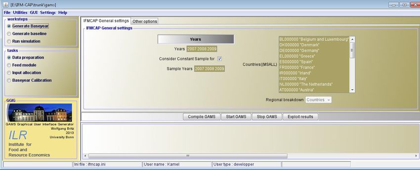
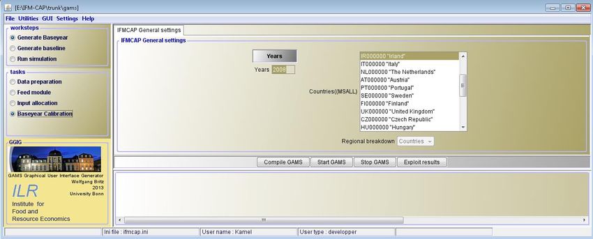
9. Graphical user interface for IFM-CAP .......................................................................... 43
10. Application of IFM-CAP to the crop diversification ‘greening’ measure ..................... 48
10.1. Baseline ............................................................................................................... 49
10.2. Crop diversification scenario .............................................................................. 49
10.3. Results ................................................................................................................. 50
10.4. Conclusions and discussion ................................................................................ 59
11. Current and future model developments ........................................................................ 61
References .............................................................................................................................. 62
Annex A: Main model parameters and equations .................................................................. 68
Annex B: Animal feed requirement functions in IFM-CAP .................................................. 83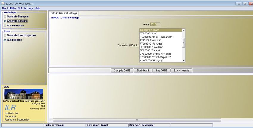
1. Introduction

Over the last two decades, the Common Agricultural Policy (CAP) has undergone a
gradual change from market intervention instruments (e.g. price support) to
decoupled farm-specific measures attempting to enhance the environmental
performance of the EU agricultural sector. This became evident with the introduction
of the Single Payment Scheme (SPS) in 2005. The 2013 CAP reform goes further in this
direction by proposing a mandatory component to direct payments, namely ‘greening’,
with the aim of supporting agricultural practices beneficial to the climate and the
environment. Other farm-specific measures introduced by the recent CAP reforms
include, among others, the capping of direct payments and young farmer and small
farmer schemes. The uptake and economic effects of these farm-specific measures
differ significantly between farms depending, among other things, on their size,
specialisation, resource endowment, location and socioeconomic characteristics.
There is a wide range of applied agricultural models available in the literature that
attempt to investigate the impact of the CAP, spanning farm-type optimisation models
to general equilibrium models (Britz, 2011; Buysse et al., 2007a; de Muro and Salvatici,
2001; Gocht and Britz, 2011; Gocht et al., 2013; Gohin, 2006; Gomez y Paloma et al.
2013; Helming et al., 2010; Louhichi et al., 2010, 2013; OECD, 2006; Offermann et al.,
2005). However, most of the models available are implemented at an aggregate level
(regions, countries, group of countries) and are not able to fully capture the impacts of
these new policy measures at a disaggregated (farm) level. Although farm-type models
can assess these farm-specific policies to some extent, they are subject to aggregation
bias, they reduce farm heterogeneity considerably and they cannot model a number of
CAP policies for which eligibility depends on individual farm characteristics and
location. For example, in the case of the crop diversification measure, certain farms
have to produce a minimum of two crops, with the main crop representing a maximum
of 75 % of the arable area. By construction, the cropping pattern is much more
diversified for a representative farm than it is for the actual individual farms on the
basis of which the representative farm was created. As a result, the crop diversification
requirement will usually be respected (not binding) at the level of the representative
farm, although in reality the restriction is binding at the level of individual farms.
Moreover, aggregated farm-group models can represent only average effects for a set of
pre-determined farm types, whereas an individual farm-level model provides the
distribution of effects over the farm population and allows the aggregation of the
results at different levels (Nomenclature of Territorial Units for Statistics (NUTS 2),
Member State (MS), EU) or by farm type (farm size, specialisation, etc.), depending on
the specific policy question to be answered.
Another drawback of existing farm models is that most of them are developed for a
specific purpose and/or location and, consequently, are not easily adapted and reused
for other applications and contexts (Louhichi et al., 2010). Out of a large number of EU-
based representative farm models, only two have full EU coverage: Common
Agricultural Policy Regional Impact Assessment Farm Type (CAPRI-FT) (Gocht and
Britz, 2011; Gocht et al., 2013) and Agriculture, Recomposition de l’Offre et Politique
Agricole (AROPAj (De Cara and Jayet, 2011). The other models cover either a specific
MS (Forest and Agricultural Optimisation Model (FAMOS) (Schmid, 2004)) or a
selected set of MSs/regions (Farm Modelling Information System (FARMIS)

                                                                                       4
(Offermann et al., 2005), Farm System Simulator (FSSIM) (Louhichi et al., 2010),
Agricultural Policy Simulator (AgriPoliS) (Kellermann et al., 2008) and Stylised Agri-
environmental Policy Impact Model (SAPIM) (OECD, 2010)).
Given the shortcomings of the available agricultural policy modelling tools, the Joint
Research Centre started developing an individual farm-level simulation model, named
IFM-CAP (Individual Farm Model for Common Agricultural Policy Analysis), for the ex
ante assessment of the medium-term adaptation of individual farmers to policy and
market changes. The main expectations from this micro-simulation tool are that it will:
(i) allow a more flexible assessment of a wide range of farm-specific policies; (ii) be
applied on a EU-wide scale; (iii) reflect the full heterogeneity (1) of EU farms in terms
of policy representation and impacts; (iv) cover all main agricultural production
activities in the EU; (v) permit a detailed analysis of different farming systems; and (vi)
estimate the distributional impacts of policies across the farm population. The typical
questions that we attempt to answer with IFM-CAP are the following: How is farm
income affected by policy reforms? Which farms would gain and which would lose?
Where are the affected farms located? What is their production specialisation? Are
small farms more affected than large ones? How many full-time and part-time jobs are
potentially affected by the policy reform?
The IFM-CAP model is a static positive mathematical programming model, which
builds on the EU-FADN data, potentially complemented by other relevant EU-wide data
sources such as the Eurostat, Farm Structure Survey (FSS) and CAPRI databases. It
consists of solving, at given prices and subsidies, a general maximisation problem in
terms of input choice and land decisions, subject to a set of constraints representing
production technology and policy restrictions. In order to reach the best
representativeness and to capture the full heterogeneity of the EU farm population, the
whole FADN farm constant sample between 2007 and 2009 (around 60 500 farms) is
individually modelled.
The IFM-CAP model starts with a simplified prototype, to which improvements will be
added at different steps of the model’s development (Table 1 summarises the main
features of this prototype). After refinement of this prototype, farm and market
interactions will be added; improvements will also be made regarding the modelling of
farm behaviour (e.g. modelling of risk and of labour and capital allocations). Finally,
additional issues such as the modelling of environmental issues and second pillar
policies will be considered (see section 11).
This report provides a detailed description of the IFM-CAP prototype in terms of
design, mathematical structure, data preparation, modelling livestock activities,
allocation of input costs and calibration process. The theoretical background, the
technical specification and the outputs that can be generated from this prototype are
also briefly presented and discussed.

(1) The Farm Accountancy Data Network (FADN) survey (therefore the IFM-CAP model) does not cover
all the agricultural holdings in the EU but only those that, because of their size, could be considered
commercial (the specific threshold varies by each MS).

                                                                                                     5
Table 1. Main features of the IFM-CAP prototype
Model name Individual Farm Model for Common Agricultural Policy Analysis (IFM-
CAP)
Institution responsible for Institute for Prospective Technological Studies (IPTS) (in-house model
development and development and maintenance) and Directorate General for Agriculture
maintenance and Rural Development (DG-AGRI)
Type of model Individual farm model running for the whole FADN sample (and
therefore all the EU regions and sectors), except farms with less than
three years’ observation during the base year period
Methodology Comparative static and non-linear programming model
Model calibration Calibrated for an average of years (3 years) using positive mathematical
programming (PMP)
Objective function Farm income maximisation: (revenues – accounting costs + pillar I
subsidies – PMP terms)
Revenues Production value by activity: price × yield activity level (ha or head)
Accounting costs Operating costs per unit of each production activity
Subsidies First pillar policies: coupling and decoupling (SPS and Single Area
Payment Scheme (SAPS))
Constraints
Land constraint Sum of area by activity less or equal to total farm land endowment
defined by type of use (arable and grassland)
Labour, capital Captured by PMP terms
Policy constraints Set-aside, quotas, greening, capping, modulation, regional ceiling for
premiums, etc.
Livestock Animal demography and livestock constraint balancing feed demand
and feed supply
Other considerations
Price, yield and subsidies Exogenous variables derived at farm level from FADN
Input costs by activity Estimated using econometric estimation (highest posterior density
(HPD) estimation with prior information derived from the DG-AGRI
input allocation module)
Total farm land endowment Fixed at base year level
Technological progress Yes, using an exogenous yield trend
Structural change No
Changes in management No
practices
Environmental indicators, No
public goods and externalities
Market interactions No
Time horizon 2020/22 (extensive use of results from Aglink/CAPRI baseline work)
Potential scenarios CAP first pillar (i.e. greening, Basic Payment Scheme, etc.); price change;
input cost change
Model results
Type of model results Production, land use, land allocation by activity within the farm, farm
income, variable costs, first pillar subsidies, distribution of income and
subsidies among farmers (base year, baseline and policy scenarios)
Farm level Single farm units
Farm group aggregation By farm typology, farm size or other relevant dimension [using farm
weighting factors from FADN (2)]
Regional aggregation FADN regions, NUTS, MS, EU
Data needs and other considerations
FADN data Constant sample single observations (2007, 2008, 2009)
Other supporting data Official statistical sources (e.g. Eurostat, FSS), scientific literature, other
models (e.g. CAPRI), etc.
Programming language General Algebraic Modelling System (GAMS)
(2) The farm weights are adjusted taking into consideration the constant sample used in the model.
6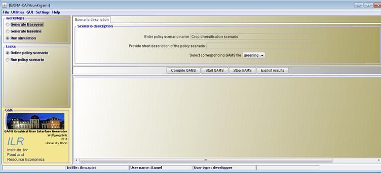
2. IFM-CAP prototype: specification and mathematical structure

IFM-CAP is a constrained optimisation model that maximises an objective function
subject to a set of constraints. For the current prototype, we have assumed that
farmers maximise their income at given yields, product prices and production
subsidies, subject to resource (arable and grassland and feed requirements) and policy
constraints such as sales, quotas and set-aside obligations. Land constraints are used
to match the available land that can be used in a production operation and the possible
uses made of it by the different agricultural activities. Constraints relating feed
availability to feed requirements are used to ensure that the total energy, protein and
fibre requirements are met by farm-grown or/and purchased feed. For certain animal
categories, additional minimum or maximum requirements by type of feeding
regarding the animal's diet are introduced.
Farm income is defined as the sum of gross margins minus a non-linear (quadratic)
activity-specific function. The gross margin is the total revenue including sales from
agricultural products and compensation payments (coupled and decoupled ( 3 )
payments) minus the accounting variable costs of production activities. The accounting
costs include costs of seeds, fertilisers, crop protection, feeding and other specific
costs. The quadratic activity-specific function is a behavioural function introduced to
calibrate the farm model to an observed base year situation (4), as is usually done in
positive programming models. This function intends to capture the effects of factors
that are not explicitly included in the model such as price expectation, risk aversion,
labour requirement and capital constraints (Heckelei, 2002).

The FADN database provides only total accounting costs per variable input category
(e.g. seeds, fertiliser, pesticide, feed, etc.), without indicating the unit input costs of
each (crop and animal) output that is needed to capture policy impacts and to
represent technologies in an explicit way. To overcome this lack of information, we opt
for a Bayesian econometric estimation of unit input costs based on the farm-level input
costs per category reported in FADN, assuming a Leontief production function (i.e.
input use increases linearly with production activity levels).
The removal of the accounting variable costs from the quadratic behavioural function
by introducing a Leontief production function for variable input costs, was motivated
by the fact that the primal technology representation through the Leontief production
function (i) provides an explicit link between production activities and the total
physical input use, (ii) eases the linkage to environmental indicator calculation, and
(iii) allows the simulation of policy measures linked to specific farm management.
According to Heckelei and Wolff (2003), the main disadvantage of this approach is the
lack of rationalisation, as intermediate input uses are assumed to be independent of
the unknown marginal costs captured by the quadratic behavioural function.
A single model template was applied for all modelled FADN farms in order to ensure a
uniform handling of all the individual farm models and their results. That is to say, all
the individual farm models have an identical structure (i.e. they have the same

(3) All farm area is assumed to be eligible.
(4) In principle, any non-linear convex function with the required properties can reproduce the base
year solution. For simplicity, and in the absence of any strong arguments for other types of functions, a
quadratic function is usually employed.

                                                                                                       7
equations and variables, but the model parameters are farm specific), and no cross-
farm constraints or relationships are assumed in the current version of the model,
except in the calibration phase, in which all individual farms in each region are pooled
together to estimate the behavioural function parameters. To render equations easily
understandable, vectors are designated by bold lower case letters, matrices by upper
case letters and scalars by italic letters. For simplicity, indices for farms are omitted.
The general mathematical formulation for IFM-CAP is as follows:
Max π p' (y x) s' x Cx d' x 0.5x' Qx (1) (5)
x 0
S.t.
(2)
Ax b ρ
where is the objective function value, x is the (N × 1) vector of non-negative activity
levels (i.e. acreages) for each agricultural activity i, p is the (N × 1) vector of product
prices (including feed and young animal prices), y is the (N × 1) vector of yields, s is the
(N × 1) vector of production subsidies (coupled and decoupled payments), C is the
(N × K) matrix of accounting unit cost for K input categories (seed, fertiliser, plant
protection, other specific costs and feeding costs), d is the (N × 1) vector of the linear
part of the behavioural activity function and Q is the (N × N) symmetric, positive
(semi-) definite matrix of the quadratic part of the behavioural activity function.
A is the (N × M) matrix of coefficients for M resource and policy constraints (land,
obligation set-aside and quotas), b is the (M × 1) vector of available resources (arable
and grassland) and upper bounds to the policy constraints, and is the vector of their
corresponding shadow prices. Product prices, yields, subsidies, set-aside rate, quotas
(sugar beet and milk) and land availability are given (i.e. derived from FADN or
estimated in the data preparation step) and are assumed to be known with certainty.
The parameters C, d and Q are estimated using highest posterior density (HPD)
estimation (Heckelei et al., 2008) (6).
In each farm and for each activity i, total production can be used for sales, on-farm use
for feeding animals or for others uses (including losses and seeding):
yi xi qi ti ui ei i 1,..., N (3)
x is the (N × 1) vector of non-negative activity levels (i.e. acreages) for each
agricultural activity i, y is the (N × 1) vector of yields, q is the (N × 1) vector of
produced quantities (i.e. production), t is the (N × 1) vector of sales/purchases
quantities (or sales/purchases of animals), u is the (N × 1) vector of used quantities for
feeding, and e is the (N × 1) vector of losses and on-farm use for seeding.
(5) The symbol indicates the Hadamard product.
(6) A detailed mathematical description of IFM-CAP prototype is given in Table A 1 in Annex A.
83. IFM-CAP database
This section provides a brief description of the data used and data treatment
procedures applied in IFM-CAP. As mentioned above, IFM-CAP is parameterised using
FADN data for the three-year average around 2008 (2007, 2008 and 2009). However,
before using the FADN data, several steps were performed in order to screen data and
to convert them to a format that is compatible with the IFM-CAP modelling framework.
This activity included in particular data adjustment to IFM-CAP model needs,
identification and correction of out-of-range values and outliers, handling missing
values and addressing the issue of variables that are not available in FADN.
3.1. Data requirement
Three types of data are required for running the first prototype of IFM-CAP: farm
resource data, input–output data for production activities, and calibration data.
(i) Farm resource data involves available farmland (i.e. total utilised agricultural area
(UAA), arable land and grassland), sugar beet quota rights and the minimum set-aside
rate. These data are used for setting lower/upper bounds for resource and policy
constraints in the model. Farmland is directly available in FADN. Sugar beet quotas are
estimated using the national share of quota because for most of the MSs these data are
not reported in the FADN database (see section 5). The set-aside rate is set to the
observed rate (i.e. the proportion of set-aside in the total area) (7). Data on labour,
energy, water and capital resources are not included, as they are not explicitly
modelled but captured by the behavioural function (i.e. PMP terms).
(ii) Input and output data for production activities consist of yields, product prices,
production subsidies and accounting unit costs for all crop and animal activities on
each farm. These data are used for the calculation of the gross margin per hectare or
per head of each production activity to be embedded in the model objective function,
as well as for the definition of input coefficients for resource and policy constraints.
The data on yields, prices and subsidies are derived from FADN. Data on accounting
unit costs for crops (i.e. specific costs related to seeds, fertilisers, crop protection and
other crop-specific costs) are estimated using a Bayesian approach with prior
information on input–output coefficients from the DG-AGRI input allocation module
(see section 4). The feeding costs are also estimated using a Bayesian approach with
prior information on animal feed requirements from CAPRI and data on farm level feed
costs, feed prices, feed nutrient contents and fodder yields from FADN, CAPRI and
Eurostat, respectively (see section 7.2). The list of crop activities defined in the IFM-
CAP model and the extraction rules for each activity are provided in Table A 3 in Annex
A. The extraction rules for the livestock activities are explained in section 6.1, as they
are more complex owing to the livestock herd demography.
(iii) Calibration data consist of activity levels (i.e. hectares or heads), rental prices, the
gross margin differential between sugar beet and the next best alternative crop and
supply elasticities at NUTS 2 level. The observed activity level (x0) is used to calibrate
(7) Note that the set-aside rate was not set to the policy rate because for some farms the observed rate is
lower than the policy rate, which can inhibit model calibration.
9the model, assuming it is the optimal crop allocation in the base year. The land rental
prices, the supply elasticities and the gross margin differential between sugar beet and
the next best alternative crop are used as prior information. Section 7 describes in
detail how these data are used in the calibration process.
Overall, most of the required data for the first prototype of IFM-CAP come directly or
indirectly from FADN with the exception of some data linked to feed crops and animal
activities (see section 6) or those used as prior information for model calibration (see
section 7) or for the estimation of sugar beet quota and prices (see section 5). For
example, the majority of calibration and farm resource data are recorded in the FADN
data and, thus, are used in the modelling exercise directly. However, some other data
such as prices and yields are not directly reported in FADN and, therefore, are derived
from the original FADN variables using simple assumptions. For example, prices are
approximated by dividing production value (TP) with the production quantity (QQ).
Production value (TP) is reported in FADN as the sum of sales, own consumption and
change of stocks, which may result in negative, very small or very large positive (i.e.
out-of-range) values for the derived prices in a given year. In fact, high carry-over
stock and a consequent drop in prices may lead to a negative total production value
and ultimately generate a negative output price. For the modelling exercise it is not
suitable to use out-of-range (i.e. negative, outliers) or zero values for prices and yields,
as they are key factors in determining the farmer’s decisions. Section 3.3 (i) describes
in detail the rule used to identify outliers and missing values for yields and prices, (ii)
provides some examples of identified outliers, and (iii) explains how we deal with
them.
The left-hand side of Figure 1 summarises the data needs of IFM-CAP and their
sources. As shown in this figure, some data are not used directly in the optimisation
process but only as prior information in the estimation procedure of certain input
coefficients.
10•FADN data
•Utilised agricultural area (arable &
grassland)
•Obligatory set-aside rate MODEL
• Sugar quota right (when available)
•Set of crop and livestock activities
•Yields, prices & subsidies
•Observed activity levels
•Farm-level feed costs
•Farm weighting factor •Optimise farm’s
•Land rental prices (prior) objectives: profit
maximisation =
linear gross margin
•EUROSTAT data – quadratic
•Yields for fodder crops at MS level behavioural
•Carcass weights function OUTPUTS
•CAPRI data •Subject to: •Activity levels
•Prices for fodder crops at MS level •Land constraints (ha & head)
•Feed prices at MS level (arable & •Production
•Feed nutrient content grassland) (tonnes)
•Prices and yields trend •Policy constraints •Land use (ha)
(CAP 1 pillar – •Input use
•Animal feed requirement functions
decoupling,
(prior) •Farm profit
quotas, set-aside,
•Elasticities for feed demand at NUTS (EUR)
greening)
2 level (prior) •Shannon index
•Feeding
constraints (feed •…
•Others data (prior) availability vs. feed
•Out-of quota prices for sugar beet requirement, max
(Agrosynergie, 2011) share of roughage
•MS sugar beet in-quota production & concentrates)
(DG-AGRI, 2014)
•In-quota prices for sugar beet
(Agrosynergie, 2011)
•Supply elasticities at NUTS 2 level ESTIMATION
(Jansson and Heckelei, 2011)
Accounting unit costs for crops
Quadratic behavioral function's parameters
Animal feed requirement & costs
Sugar beet quota & prices
DATA
Figure 1. IFM-CAP prototype description
3.2. Selection of farm constant sample
A constant sample of farms for the base year period 2007–2009 is selected and stored
in a single file to facilitate data management. Figure 2 shows the number of farms in
the constant sample. In the EU-27 (8), of the total 81 114 farms sampled in 2007, only
(8) In the IFM-CAP model, Belgium and Luxembourg are grouped together as one country (indicated by
BL) because of data availability (trade data) and the similarity of their agriculture.
1160 552 remained in the sample until 2009. The proportion of farms that remain in the
constant sample varies strongly across MSs.
EU-27
2007
81 114
from 2007 (nr holdings)
2008
66 652 11 283 from 2008 (nr holdings)
from 2009 (nr holdings)
2009
60 552 9 218 10 609
0 20 000 40 000 60 000 80 000 100 000
Figure 2. Evaluation of the number of FADN farms in the EU-27
The FADN is a representative stratified sample with regard to regional disaggregation
(FADN regions), production specialisation and farm size. An individual weighting
scheme is applied to each farm in the sample corresponding to the number of farms it
represents in the total population. The weighting scheme allows aggregation of results
at different regional levels (e.g. NUTS 2, MS, EU level) or by farm type according to
specialisation, farm size, etc. Because we consider the constant sample, the weights
need to be adjusted in order to account for the farms in the FADN sample that are
excluded from the final database used in IFM-CAP. The adjusted weights (indicating
the number of farms represented in each dimension cell as the combination of region,
economic size and type of farming) will be used in particular for (i) the calculation of
the three-year averages around 2008, used as base year, (ii) the calculation of average
data at NUTS 2 level to be used during the data preparation routine for handling
missing values, and (iii) the aggregation of model results by region (NUTS 2, MS and
EU) and by farm type (specialisation, size).
3.3. Data screening and treatment
The purpose of the FADN data screening is to remove aberration and to check to what
extent these data need to be adjusted to reflect the IFM-CAP modelling requirements.
The key data that have been screened are: yields, product prices, production quantities
and production values. The data screening involves two steps: (i) detecting and
handling outliers; and (ii) identifying and addressing the problem of zero/missing and
negative values. The data treatment was applied to the raw data before averaging them
over the three years considered in the model.
Outliers
Outliers are observations that are numerically distant from the rest of the data. In our
case, they concern mainly prices and yields and may originate for various reasons:
12 Because prices and yields are derived from other FADN data (based on total
production value, production quantity and areas), their values in some farms may
deviate significantly from the rest of the sample if underlying data do not portray
sufficient information to identify their true value (e.g. because of high carry-over
stock combined with a high price (9)). The formulas for price and yield calculation
are given as follows:
Prices are derived as: p = TP / QQ
Yields are derived as: y = QQ / AA
where TP is production value (euros); QQ is production quantity (tonnes); AA is
production area (hectares)
TP is calculated as: TP = SA + FC + FV - (BV - CV)
where SA is sales; FC is farm consumption; FV is farm use; BV is opening stock;
CV is closing stock
Because of high heterogeneity in yields and prices for specific activities included in
a given aggregated activity group (e.g. flower (FLOW), other cereals (OCER), other
vegetables (OVEG)), as well as for crops with yields strongly dependent on climatic
conditions or variety cultivated (e.g. tobacco (TOBA), potatoes (POTA), olives
(OLIV), and pasture (GRAS)).
Because farmers may have imputed incorrect information in particular for output
quantity and/or output value in the FADN farm returns.
In the case of yields, the outliers were kept unchanged. This was motivated by the fact
that there can be high yield heterogeneity owing to variation in the natural conditions
(e.g. soil type, weather effects, infections and diseases) and management practices (e.g.
irrigation, crop variety, input application).
For prices, normality tests have been carried out, and for consistency we have used a
non-parametric method (the interquartile range (IQR)) for determining and replacing
the outliers in prices.
The IQR is a measure of statistical dispersion, being equal to the difference between
the upper and lower quartiles:
This data treatment was conducted at NUTS 2 level. More precisely, it is a trimmed
estimator, defined as the 25 % trimmed mid-range, and it is the most significant basic
robust measure of scale. It is the third quartile of a box and whisker plot minus the first
quartile. An outlier is defined as any value that lies at more than one and a half times
the length of the IQR, therefore:
( )
(9) The opening valuation is based on the value of the stocks at the start of the accounting year at farm
gate prices current at that time.
13( )
We have identified a total of 27 788 upper outliers and 12 197 lower outliers for prices
representing around 7 % of the total number of prices for the three years (2007–
2009).
We have analysed two options of treating outliers: discarding (trimming) and
winsorising (transforming). As the number of outliers was large and in order to keep
the FADN sample intact, we have decided to transform the (lower/upper) outliers
using the values of the (lower/upper) outlier threshold defined as follows:
Lower outlier threshold = Q1 - 1.5×IQR
Upper outlier threshold = Q3 + 1.5×IQR
The IQR is equal to the difference between the upper (Q3) and lower quartiles (Q1)
defined at the NUTS 2 level:
IQR Q3 Q1
Variables with zero and negative values
FADN assigns zero values to variables for which data is not collected. For this reason it
is often difficult to distinguish between a variable with a missing value and a variable
with an observed zero value. We treat all zero values for existing (non-zero) activity
levels as ‘missing values’ in our data management tool and replace them with a specific
value when necessary.
Three crucial FADN variables are used for calculating prices and yields: total
production value (TP); output quantity (QQ); and areas (AA). In the first step, all the
negative values associated with output quantities and areas have been substituted by a
zero value. After conducting this procedure, a total of 123 236 ‘missing’ (zero) values
were identified for TP and QQ over the three years considered in the model. This
represents around 20 % of crop activities for which activity level – area (AA) – is non-
zero. Because prices and yields are derived from total production and output quantity,
their value cannot be calculated. In addition, 1 486 variables (representing 0.20 %) are
identified with negative total production value (TP) (therefore price). To address this
problem, we have implemented the following corrections:
1. Total production (TP) is ‘negative’: we set crop prices to the average price at the
NUTS 2 level. If the NUTS 2 prices are not available, we use average national prices.
Next, we recalculate total production value (TP) based on the new price and the
reported output quantity (QQ).
2. Total production (TP) is ‘missing’: if output quantity (QQ) is positive while total
production value (TP) is missing, we set crop prices equal to the average crop price at
NUTS 2 level, assuming that prices cannot be equal to zero. If the average regional
prices are not available, we use average national prices. Next, we recalculate total
production value (TP) based on the new price and the reported output quantity (QQ).
143. Output quantity (QQ) is ‘missing’: if activity level/area (AA) and total production
value (TP) are available, while output quantity (QQ) is not, we set crop yield equal to
the average regional (NUTS 2) yield, recalculate the output quantity (QQ) based on the
new yield, and recalculate the price based on the total production value (TP) and new
output quantity (QQ). As above, if the average regional yields are not available, we use
average national yields.
4. Output quantity (QQ) and total production (TP) are ‘missing’: if activity level/area
(AA) exists, while total production value (TP) and output quantity (QQ) are not
available, we set crop prices equal to the average regional price (10) and crop yield
equal to zero. We assume that production/yield can be equal to zero but not prices. In
cases in which the average regional price is not available, we use the average national
price.
3.4. Extraction rules for subsidies
The current version of the IFM-CAP prototype relies fully on subsidy data available in
FADN. The FADN (and thus also IFM-CAP) covers both coupled and decoupled CAP
payments. The coupled payments for crops (SUBCRO) include compensatory payments
for annual and permanent crops (SUBCRO_COP), set-aside (SUBCRO_SETA), other
specific crop payments (SUBCRO_OTHER) and other coupled subsidies (SUBART) (11).
The decoupled payments (SUBDEC) include Single Payment Scheme (12) (DPSFP), Single
Area Payment Scheme (DPSAP) and additional aid (DPAID). Rural Development
Subsidies are not included in the model at this stage (Table 2 and Table 3).
Coupled crop payments are distributed to eligible crops (13). They are calculated per
hectare for each eligible activity based on area proportions in the total eligible area.
This means that in cases where there is more than one activity benefiting from the
payment (e.g. DPCER), subsidies are distributed over all eligible activities using the
area proportions. In the special case in which all eligible activities have ‘zero’ area in
the database, the payment is distributed to all farm activities using the area
proportions as the distribution key.
In the livestock sector, four types of coupled animal payments are considered: dairy
subsidies (SUBLIV_DAIR), other cattle subsidies (SUBLIV_OTCA), sheep and goat
subsidies (SUBLIV_SHGO) and other livestock subsidies (SUBLIV_OTHER). Given that
these subsidies are distinguished by livestock type (cattle, sheep and goat, etc.) and
animal category (cows, heifers, male cattle, etc.), they are calculated per head. As in the
arable sector, they are distributed over eligible animal activities based on the
proportion of each eligible activity in the total number of animals benefiting from these
payments. Table 3 summarises the rules used for the extraction of animal subsidies
from FADN.
(10) When replacing prices or yields for a single year with an average price/yield, we calculate the
deviation from average prices/yields for the other two years and adjust assigned average price/yield by
the average deviation for the two years.
(11) The extraction rules for the subsidies follow in part the ones implemented in FADNTOOL. Other
coupled subsidies include those granted under the Article 68 of Regulation (EC) No 73/2009.
(12) Often referred to as Single Farm Payment.
(13) The crop and livestock activities benefiting from each payment (and by year) are specified in Table
A 6 in Annex A.
15Table 2. Extraction rules for coupled crop payments and decoupled payments
from Table J and M in FADN
FADN
Categories subsidies GAMS acronym s Extraction rule
Table
Coupled payments SUBCRO J+M
M (602CP...614CP) +
Compensatory payments per area SUBCRO_COP M M618CP + M(622CP...629CP) +
M(632CP...634CP) + M638CP + M655CP
Set-aside premiums SUBCRO_SETA M M650CP
JC(120...145) + JC146 + JC(147...161) + JC185 +
Other crop payments SUBCRO_OTHER J JC(281...284) + JC(296...301) +
JC(326...357) + JC(360...374) + JC952
Art. 68 subsidies SUBART J JC956
Decoupled payments SUBDEC J JC670 + JC680 + JC955
Single farm payment DPSFP J JC670
Single area payment DPSAP J JC680
Additional aid DPAID J JC955
16Table 3. Extraction rule for coupled animal payments
Subsidies GAMS GAMS
Description Extraction rule
in FADN acronym acronym.
Direct payments to dairy
DPDCOW M770CP
Subsidies cows
SUBLIV_DAIR
dairying Other payments to dairy
JCDOW JC30 + JC32 + JC163
cows
Special premiums to bulls
DPBULF M710CP
and steers
Direct payments to suckler
DPSCOW M731CP
cows
Additional payments to
DPNE_MEAT M735CP
bovine meat cattle
Slaughter premium for adult
DPSL_ADCT M742CP
cattle
DPSL_CALV Slaughter premium for calves M741CP
Subsidies Additional payments
DPADDPNA M760CP
other SUBLIV_OTCA (national envelope)
cattle Extensification payment for
DPEXTENS M750CP
bulls, steers and suckler cows
JCBULF Payments bull fattening JC25 + JC27
JCSCOW Payments suckler cow JC32
JCHEIR Payments heifers raising JC26 + JC28
JCHEIF Payments heifers fattening JC29
JCCAR Payments calves raising JC24
JCCAF Payments calves fattening JC23
JCCATT Payments cattle JC52 + JC307
JCOCAT Other payments other cattle JC31
Payments sheep and goat
Subsidies JCSHGO JC54 + JC55 + 308
fattening
sheep and SUBLIV_SHGO
Payments sheep and goat
goats JCSHGM JC38 + JC40 + JC(164….JC168)
milk
JCPIGF Payments for pig fattening JC45 + JC46
JCPIGS Payments for pigs and sows JC309 + JC56
JCSOWS Payment for sows JC44
Subsidies JCHENS Payments for hens JC48 + JC169 + JC43
on other SUBLIV_OTHER JCPOUF Payments for poultry JC47 + JC49 + JC310
livestock Payments for hens and
JCPOU JC57
poultry
JCOANI Payments for other animals JC50 + JC58
JCOTHLI Other payments livestock JC951 + JC170 + JC171 + JC311
For the decoupled payment (i.e. SUBDEC), we calculate the payment value on each
farm on the basis of the received decoupled aid and the number of eligible hectares. All
the eligible area on each single farm receives a uniform per hectare decoupled
payment (Table 2).
4. Input cost estimation
FADN collects the monetary value of crop inputs, livestock inputs and other farm costs
(e.g. overheads, depreciation, hired labour costs, interest costs) at farm level.
17Information on how these aggregate costs are distributed over specific farm activities
is not recorded. Starting from the reported farm-level aggregate input costs, we
therefore estimate activity-specific unit input costs using a Bayesian econometric
approach (14). The resulting estimated accounting units costs for K input categories
(seed, fertiliser, plant protection and other specific costs) are directly incorporated in
the model's objective function () as the elements of the matrix C (N × K) in equation
(1) above.
4.1. Leontief technology specification
For the estimation of input costs, we assume a Leontief production function for
intermediate inputs (i.e. input use increases linearly with the production activity
levels). Such a linear input demand equation has been used widely in the literature
(e.g. Léon et al., 1999; Kleinhanss et al., 2011). This allows us to link production
activities and total physical input use. However, the rigid technology assumption and
the failure to consider, for example, soil quality and crop rotation effects in input use
can be a serious limitation. One common way to handle these problems and make the
technology set more flexible, without departing from the Leontief specification, is to
include activities with discretely varying input intensities.
Hence, input allocation is assumed to display the following linear relationship to
output:
z Ηv u (4)
where z is the (K × 1) vector of input costs, v is the (N × 1) vector of total value of
outputs, H is an (N × K) matrix of unknown input–output coefficients and u is the (K × 1)
vector of random errors.
This relationship can be expressed by farm and input category as follows:
z f,k H i,k v f ,i u f , k (5)
i
where is the total (explicit) cost of variable input k (k = 1,…, K) for farm f (f = 1,
…, F) recorded in FADN, is the total value of output i (I = 1,…, N) for farm f, is
the expenditure on input k required per unit of output value i and is a random
disturbance term which is specific to each input category and to each farm (Errington,
1989). It is assumed that farms within the same region and the same farm type have a
common technology, and thus the same input–output coefficients (i.e. the index for
farm types is omitted here).
In order to ensure that the accounting balance between total revenue and total cost is
respected, the following accounting restriction is imposed for each output i:
H
k
i .k 1 (6)
(14) In parallel, an alternative way of estimating the costs of production is being tested, making use of the
cost function approach, which would alter the entire modelling approach (see section 11).
18Following Léon et al. (1999), this is achieved by introducing a residual input category
‘value added’ with corresponding monetary input coefficients equal to the difference
between the total revenue and the sum of all other monetary input coefficients across
input categories. Similar to other input categories, value added is restricted to being
positive, assuming that, for each type of output i averaged (across all farms) total cost
cannot exceed total revenue.
4.2. Highest posterior density estimation
In order to select the most accurate method for estimating the unknown input–output
coefficients , we have tested several alternative estimation approaches for a
sample of 565 farms in a region in France, for which details on activity-level input
costs were recorded. We aggregated the crop-specific input costs at farm level, and
tested the performance of different methods (including seemingly unrelated
regressions (SURs), entropy and highest posterior density (HPD) estimation) in
recovering the true disaggregated crop-specific input costs (for details on these
alternative estimation approaches and their performance, see Colen et al., 2014). As
prior information for the entropy and HPD approach, we propose the use of the results
of the input allocation key that was developed by DG-AGRI and we compare this with
alternative types of prior information that were proposed in earlier studies. The key
allocates total accounting costs to individual output activities based on the proportion
of activity output value in the total output value (for details see Table A 7 in Annex A).
Several accuracy criteria showed that the HPD approach, using the inputs allocated
according to the input allocation key as prior information, performed best. HPD also
has a significantly lower computational demand, which is non-negligible given the
large sample of individual farms in the IFM-CAP model.
Hence, we estimate the input–output coefficients, H, by NUTS 2 region and farm type,
using the HPD approach and prior information ̅ based on the input allocation key
developed by DG-AGRI. The HPD approach minimises the normalised least square
deviation between the estimated input–output coefficients and the prior information.
This Bayesian approach was proposed by Heckelei et al. (2005) as an alternative to
entropy methods for deriving solutions to underdetermined systems of equations.
They argued that the main advantage of this approach is that it allows a more direct
and straightforward interpretable formulation of available a priori information and a
clearly defined estimation objective. In the HPD estimation the model parameters are
treated as stochastic outcomes. In this context, the method distinguishes between the
prior density, p(H), which summarises a priori information on parameters, and the
likelihood function, L(Hv), which represents information obtained from the data in
conjunction with the assumed model. The combination of the prior density and the
likelihood function results in a posterior density that can be expressed as (e.g. Zellner,
1971, p. 14).
z(Hv)(p(H)L(Hv)) (7)
where z denotes posterior density, is the proportionality, H are the parameters to
estimate and v is the vector of observations. This approach is extensively discussed in
Heckelei et al. (2008). This leads to the following estimation problem:
19( ̅) ∑ ( ̅)
Subject to:
(8)
where ̅ contains the prior values and HPD is the prior density function of the form
vec(H) ~ N(vec( ̅ ),∑). The prior values, ̅ , are the mean input–output coefficients
by NUTS 2 region and farm type, obtained through DG-AGRI's input allocation key (see
Table A 7). The covariance matrix, ∑, is set equal to a diagonal matrix with elements
twice the variance of the input–output coefficients obtained from the input allocation
key method: (2σH)². For the error term, u, we use a prior density function of the form
N(0,∑), with prior mean zero and with twice the squared standard deviation of the
error (2σu)² as elements of the diagonal covariance matrix. For more details, refer to
Table A 3 in Annex A.
The solution to this optimisation problem provides estimates for the unknown input–
output coefficients, , for each region and farm type and for the error term, u.
This approach does not ensure that all input costs are fully distributed over activities.
Therefore, for each farm we proportionally allocate the remaining non-distributed
costs across the different activities, leading to a farm-specific corrected input–output
coefficient, ̃ . These corrected input–output coefficients ensure that aggregate
input costs are completely distributed, and further improve the accuracy of input cost
estimates (see Colen et al., 2014). Based on these corrected coefficients, ̃ , and the
value of production per observed activity level, , the unit input costs of the
matrix C (N × K), i.e. the input costs per hectare of activity i, can be calculated as
follows:
~ z f ,k
H f ,i,k H i ,k
H
i
i ,k v f ,i (9)
n n
~
z f,k H f ,i,k v f ,i C f ,i,k x 0f ,i (10)
i 1 i 1
Hence,
̃ (11)
20For illustration, the resulting average estimated input costs per hectare, , are
reported for each crop and input cost category in Table A 8 (Annex A) for the regions
Burgundy and Andalusía.
5. Estimation of sugar beet quota
The common market organisation for sugar is subject to production controls
implemented by a system of supply quotas. The quotas are defined for each MS, which
allocates the quota to sugar refineries, which in turn allocate ‘delivery rights’ to
individual farms. The quota specifies the amount of ‘quota beet’ (in-quota sugar beet)
farms can deliver at supported prices. Any quantities sold beyond the quota (out-of-
quota sugar beet) have to be sold at international prices and thus they receive a lower
price than the in-quota beet (Agrosynergie, 2011; Burrell et al., 2014; European
Commission, 2013).
The IFM-CAP cannot fully rely on FADN data for modelling the sugar beet quota
system. The FADN contains records on sugar beet area (K131AA), total sugar beet
production (K131QQ (15)), average sugar beet price (p) (K131TP/K131QQ) and sugar
beet in-quota quantity (L421I). Although there are data available on sugar beet quota
(L421I) for several MSs (i.e. Austria (AT), Belgium-Luxembourg (BL), Germany (DE),
Lithuania (LT), the Netherlands (NL), Poland (PL), Spain (ES), Sweden (SE) , Greece
(EL) and the United Kingdom (UK)) (16), their quality needs to be considered carefully.
Only in four MSs (i.e. Belgium-Luxembourg, Germany, Lithuania and Poland) is the
ratio between the reported MS sugar quota (DG-AGRI, 2014) and the quota in FADN
(aggregated at MS level using the farm weights for the average year) within a
reasonable range, i.e. between 0.5 and 1.5 (17). This implies that the data for in-quota
prices, sugar beet quota and out-of-quota prices, which are indispensable for the
modelling of quota regime in IFM-CAP, cannot be fully recovered from FADN and need
to be estimated and/or extracted from other data sources. Other potential data sources
available for the entire EU that can supplement the FADN data include FSS and DG-
AGRI (see Table A 12).
Table A 13 provides a comparison of the (weighted) FADN data with the FSS data for
area, production and yield of sugar beet averaged for the years 2007–2009. On
average, FADN reports higher values (for production and area) than FSS (by around
25 %), implying that sugar beet is over-represented in the FADN sample compared
with the total population (18). There are some MSs in which this difference is very
large. For example, for Spain and Romania the sugar beet area in FADN is 108 % and
(15) The reported quantity is net of sugar beet tops.
(16) It has been assumed that the reported quota data is in sugar beet (instead of sugar).
(17) The ratio between the MS quota reported by DG-AGRI (DG-AGRI, 2014) and the one in FADN is the
following: EL = 0.00; BL = 1.42; DE = 1.26; ES = 1.59; LT = 1.12; NL = 0.18; AT = 49.67; PL = 0.63;
SE = 0.30; UK = 2.76.
( 18 ) The explanation could be that the FADN covers only commercial farms and that the
representativeness of the FADN sample is constructed from location of the farm (region), economic size
and type of farming and not from each production activity. Hence, the FADN may not be representative
with respect to each activity (e.g. sugar beet production).
21You can also read