The Local Technology Spillovers of Multinational Firms
←
→
Page content transcription
If your browser does not render page correctly, please read the page content below
The Local Technology Spillovers of Multinational Firms
                                       Robin Kaiji Gong
                        The Hong Kong University of Science and Technology1

Abstract

This paper identifies the causal effect of U.S. multinationals’ technology shocks on their
subsidiaries’ and nearby domestic firms’ productivity in China. By combining firm-level
data from both the U.S. and China, I match U.S. multinationals with their manufacturing
subsidiaries in China and measure the multinationals’ technology shocks to the local firms
in China based on the multinationals’ patenting activities in the U.S. To address potential
endogeneity concerns, I introduce an instrumental variable strategy based on U.S. state-level
R&D tax credit policies. I find multinationals’ technology improvements induce an increase
in the value-added output and total factor productivity (TFP) of both their own subsidiaries
and domestic firms in the local areas. The size of the local technology spillover effect depends
on local firms’ absorptive capacity. I further provide evidence of spillovers through produc-
tion linkages as well as technological linkages. In addition, spillovers through technological
linkages also stimulate innovation of the productive local firms.

Keywords: FDI, technology spillovers, patents, productivity.
JEL codes: D2, F2, O1, O3

1
    Email: rkgong@ust.hk. I thank Nicholas Bloom, Pete Klenow, Kyle Bagwell, and Hongbin Li for their
    dedicated discussions and guidance. I also thank Caroline Hoxby, Pascaline Dupas, Isaac Sorkin, Daniel
    Xu, Matilde Bombardini, Heiwai Tang for their detailed suggestions and comments. I thank all seminar
    participants in Stanford University. Financial support from the Stanford Institute for Research in the Social
    Sciences Dissertation Fellowship and the Stanford Institute for Economic Policy Research Dixon and Carol
    Doll Graduate Fellowship is gratefully acknowledged.

Preprint submitted to Elsevier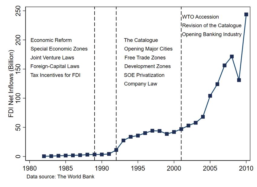
1. Introduction

      Foreign affiliates of multinational corporations (MNCs) accounted for 12% of global pro-
duction in 2014.2 MNCs’ expansion during the past several decades has been accompanied
by a lengthy debate over their role in the global economy, particularly in developing coun-
tries. In principle, international knowledge diffusion stimulates global economic growth and
drives productivity convergence between developing and developed countries (Romer (1993),
Coe et al. (1997)). Multinational activities are one of the primary channels through which
technology is disseminated globally (Keller (2004)): through the sharing of technology be-
tween multinational parents and their foreign subsidiaries, technological advances in multi-
nationals’ home countries are then transmitted to foreign destinations (Markusen (2004)).
Macro-level evidence (Borensztein et al. (1998)) has also suggested foreign direct investment
(FDI) contributes to the economic growth of developing countries. Potential gains from
MNCs’ technology spillovers have encouraged governments to adopt FDI incentive policies,
such as tax incentives, financial subsidies, and regulatory exemptions in many developing
countries.
      However, the micro-level evidence of technology diffusion through multinational activities
remains mixed and inconclusive (Harrison and Rodrı́guez-Clare (2010)). Previous studies
have often documented the impact of FDI inflows on domestic firms in the same industries to
be neutral (Haddad and Harrison (1993)) or even negative (Aitken and Harrison (1999)). On
the contrary, domestic firms in upstream industries may benefit from FDI inflows through
backward linkages (Javorcik (2004)). The role of technology remains obscure in previous
literature: horizontally, the potential productivity gains could be offset simultaneously by
the competition of multinational entries, while vertically, distinguishing production efficiency
improvements from potential supply or demand shocks is difficult.
      This paper aims to fill the gaps in the literature by examining the impact of multination-
als’ technological improvements on their subsidiaries and domestic firms in nearby geographic
areas. I first match U.S. public companies with their subsidiaries in China based on the in-
formation provided in their annual financial reports (10-K files). I then measure the impact

2
    “Multinational enterprises in the global economy”, OECD Report.

                                                     2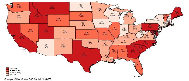
of the technology shocks from these parent companies to their subsidiaries based on the
citation-weighted patent stocks of the parent companies. I further construct the technology
shocks of the MNCs to the domestic Chinese firms in nearby geographic areas as a weighted
sum of the parent-subsidiary technology shocks. To address potential endogeneity problems,
I adopt an instrumental variable strategy based on state-level research and development
(R&D) tax credit policies in the U.S., which induce exogenous shocks to firms’ innovation
incentives (Wilson (2009), Bloom et al. (2013)). The primary analysis focuses on three sets
of outcome variables: value-added output, revenue-based total factor productivity estimated
following Ackerberg et al. (2015), and labor productivity measured in terms of value-added
per worker.
   This paper establishes two main results. First, technological advances of U.S. multi-
nationals are transmitted to their foreign subsidiaries and improve the value-added output
and productivity of these subsidiaries. Second, the technology improvements are further
transmitted to domestic firms that are geographically close to the subsidiaries, thereby pre-
cipitating production expansions and productivity growth of domestic firms. The results
validate the existence of both technology transfers from parent companies to their foreign
subsidiaries within MNCs, and local technology spillovers from the MNCs to domestic firms.
Further discussion reveals the revenue-based productivity improvements are likely to be
driven by production efficiency gains rather than price fluctuations. The magnitude of the
local technology spillover effect also hinges on local firms’ human capital stock, product in-
novation activities, and ownership types, which are related to the absorptive capacity theory
in the management literature (Lane and Lubatkin (1998)).
   To advance our understanding of the local technology spillover effects, I further inves-
tigate the impact of technology shocks through production linkages. I demonstrate that
multinationals’ technology shocks lead to production expansions and productivity gains in
the domestic firms in both upstream and downstream industries, whereas the effect on firms
in the same industry is positive but statistically insignificant. The results suggest multi-
nationals’ technological improvements would diffuse to the nearby domestic firms through
the production networks, consistent with the findings in the previous literature (Javorcik
(2004)).

                                              3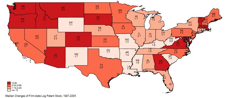
I further construct measures of technology shocks based on the technological similarity
between MNCs and local industries (Hall et al. (2001)), as ordinary industry classification
might be insufficient to capture the extent of technology spillovers. I find local firms with
closer technological linkages to the multinationals realize higher productivity gains from
such spillovers. Technology shocks through technological linkages also stimulate innovation
activities of the more productive firms in the local areas.
      This paper contributes to the literature on the following grounds. First, it supplements
prior studies on the relationship between multinational parents and foreign subsidiaries.
Models of multinational production have commonly presumed multinational parents and
foreign subsidiaries share common technological inputs (Helpman (1984), Markusen (1995),
Helpman (2006), and Antras and Yeaple (2014)). Meanwhile, empirical research has sug-
gested the existence of technology transfers from multinational parents to their foreign sub-
sidiaries in the form of patent royalty transactions (Branstetter et al. (2006)) and that
intra-firm technology diffusion further enhances multinationals’ sales growth in the foreign
market (Keller and Yeaple (2013), Bilir and Morales (2018)). This study complements pre-
vious theoretical frameworks and empirical findings by providing direct causal evidence of
multinational subsidiaries’ productivity gains as a result of their parents’ technology ad-
vances.
      The results also shed light on empirical studies on multinationals’ spillover effects. Indus-
try shares of employment and output in foreign-owned firms are frequently used as common
proxies of multinational spillovers in the previous literature. Based on those measures, on
one hand, studies such as Haddad and Harrison (1993), Aitken and Harrison (1999), Djankov
and Hoekman (2000), Konings (2001), Bwalya (2006), and Tao et al. (2017) report that for-
eign capital inflows exert a minimal or negative effect on the productivity of domestic firms
in the same industry;3 conversely, domestic firms in the upstream industries are likely to
benefit from foreign capital inflows, suggested by studies including Javorcik (2004), Kugler
(2006), Blalock and Gertler (2008), Javorcik and Spatareanu (2008), Javorcik and Spatare-
anu (2011), and Gorodnichenko et al. (2014). The classic approach is appealing in that it

3
    For developed countries, however, studies such as Haskel et al. (2007) and Keller and Yeaple (2009) find
    positive horizontal FDI effects.

                                                      4
reflects the overall impact of multinational activities, but it may also embed challenges for
precise interpretation and causal inference of the spillover effects (Keller (2004)). This paper
complements the previous studies through the following means. First, rather than relying
upon the FDI employment shares, I directly use the parent companies’ patent filings to infer
potential technological diffusion to their subsidiaries and domestic firms,4 . Second, I intro-
duce an identification strategy that relies on policy changes in the home countries.5 Because
the R&D tax credit policy in the U.S. is unlikely to be driven by multinationals’ performance
and foreign market fluctuations, the strategy provides an opportunity to identify the causal
effect of multinationals’ technology spillovers on the domestic firms in other countries.
Lastly, my analysis also relates to research in the innovation literature. First, studies
including Henderson et al. (1993), Peri (2005), Henderson et al. (2005), Thompson (2006),
Agrawal et al. (2008), and Murata et al. (2014) illustrate that knowledge spillovers (measured
by patent citations) are substantially limited by distance.6 I incorporate the insights into
the paper by restricting my analysis to the domestic firms that are geographically close
to the multinational subsidiaries. Second, as discussed in Schmookler (1966), Jaffe (1986),
and Griliches (1992), the product-based industry classification system is often insufficient to
represent technological boundaries, and the industry technology shocks based on technology
linkages adopted in this study improves upon the previous sectoral FDI spillover measures
by linking MNCs’ knowledge stocks with their relative importance in the Chinese industries.
Third, my results also contribute to previous research concerning the real effect of innovation
(Jones and Williams (1998), Hall et al. (2010), Hall (2011)) by connecting the innovation
outcomes of multinationals with the productivity of the foreign subsidiaries and domestic
firms.
The paper is organized as follows: Section 2 introduces the data and construction of key
variables. Section 3 outlines the main specification and introduces the identification strategy.
4
An example of using patent data to measure technology spillovers is Bwalya (2006) in which citation counts
are used to infer technology spillovers from Japan to the U.S.
5
Some recent studies also adopt other identification strategies. For example, Tao et al. (2017) utilizes changes
of FDI restrictions in China after 2001 for identification; Abebe et al. (2018) exploits the natural experiment
of FDI entry in the local districts.
6
Macro-level analysis such as Keller (2002) also suggests the benefits from R&D spillovers are decaying over
distance.
5Section 4 presents the baseline results as well as the related robustness checks and discussion
of firms’ absorptive capacity. Section 5 examines the technology spillover effects through
production linkages and technological linkages, and discusses local firms’ response in their
innovation activities. Section 6 concludes.
2. Data and Variable Construction
2.1. Institutional backgrounds
The Chinese Economic Reform of 1978 aimed to transform a central government planned
economy into a market economy. The reform was initially accompanied by policies that
opened certain regions in China to international trade and foreign investment. Since 1980,
the government has established several designated economic zones that allow for foreign
investment, including cities such as Shenzhen, Zhuhai, Xiamen, Shantou, and the entire
Hainan Province. During the 1980s, the Chinese government also passed joint venture laws
and foreign-capital laws to support an institutional environment that protects the property
rights of foreign investors. The reform was reinforced after 1992, when Deng Xiaoping re-
affirmed continuation of the economic reform during his southern tour. Between 1993 to
2000, the government opened major cities such as Beijing and Shanghai to trade and foreign
investment and further minimized tariffs and trade barriers. In 1995, the government pub-
lished the “Catalogue for the Guidance of Foreign Investment Industries” (“the Catalogue”),
a guide for the local governments to encourage, permit, restrict, or prohibit FDI in certain
classified industries. The industry classification underwent several rounds of revision after
2000. The net inflow of FDI skyrocketed in China after 2001, when the country joined the
World Trade Organization (WTO); the figure increased from less than 50 billion in 2001 to
about 250 billion in 2010. Figure 1 illustrates the growth of U.S. FDI inflows and the major
policy events in China between 1978 and 2010.
U.S. multinationals’ FDI in China was initiated early during the Chinese market reform.
The U.S. and the People’s Republic of China established diplomatic relations in 1979, and
in the following several years, numerous U.S. MNCs established their first subsidiaries in
6Figure 1: Institutional Background
Notes: This figure shows the change of FDI net flows into China and the corresponding policy changes during
the same period. The figure divides the evolution of the institutional changes into three major periods. The
first period starts from 1982 to 1989, when China started its market economy reform and opening to trade
and FDI. The second period starts from 1992 to 2001, when China deepens the market reform by enriching
the ownership laws, opening major cities and trade zones, and starting the privatization process of SOEs.
The third period starts from 2001 to 2010, when China accesses WTO and becomes the world’s major
destination of FDI.
China, including Coca Cola (1979), Pepsi (1981), Johnson & Johnson (1982), and Hewlett-
Packard (1985).7 Although these early entrants often opted for a Chinese headquarters in
major cities such as Beijing, Shanghai, and Guangzhou, they have expanded operations to
the other cities later. For example, Pepsi first established its headquarters in Beijing in
1981; however, as of 2000, it has established production factories in regional centers such
as Changchun, Chongqing, Guilin, Nanchang, and Nanjing. Following the growth of U.S.
multinationals’ Chinese businesses, the U.S. also became the third largest source country of
FDI in China in 2006 (excluding the tax havens) following Japan and South Korea. In 2006,
the total amount of FDI inflow added up to 3,061.23 million.8
Rich anecdotal evidence has suggested foreign direct investment is likely to introduce
technology spillovers to local companies in China. For decades, the Chinese government has
7
See Table A1 for examples of U.S. multinationals and their entry years.
8
See Table A2 for the major origins of FDI inflows in China.
7been accused of its implicit “technology for markets” policy, under which foreign companies
are required to transfer technology to domestic firms to initiate operations in China.9 Mean-
while, domestic firms may imitate or reverse engineer the products and technology of the
multinationals. Foreign companies may also voluntarily share technology with local firms
to prevent hold-up problems with local suppliers (Blalock and Gertler (2008)). Technology
spillovers may also exist in many other forms, such as labor pooling (Poole (2013)).
2.2. Data sources and variable construction
The Chinese data used in this study are based on the Annual Survey of Industrial En-
terprises (ASIE), which are collected by the Chinese National Bureau of Statistics (NBS)
and includes all state-owned enterprises (SOEs) and non-SOEs with annual sales of over
5 million Chinese yuan (about $604,600 in 2000). The data contains basic information of
each company, including name, location, industry, ownership structure, and starting year;
and performance variables, such as gross output, value added, net income, fixed assets, in-
termediate inputs, and employment. Some items that are uncommon in standard financial
statements are also reported in the ASIE, including value of export, value of new prod-
ucts, and employee compensation. I primarily focus on two sets of key firm-level outcome
variables: value-added output and revenue-based productivity measures (total factor pro-
ductivity and labor productivity). Value-added output is constructed directly based on the
data using the logarithm of the reported values, deflated by industry price indices. I fur-
ther estimate a two-factor production function (Ackerberg et al. (2015)) with value added
as production output and employment and capital as production inputs,10 to estimate the
revenue-based total factor productivity (TFPR).11 I also construct labor productivity defined
by log value-added output per worker as well as other firm-level outcome variables from the
data, including wage, return on assets (ROA), intangible assets, and value of exports. The
other Chinese data sources used in this study include Chinese patent data from the State
Intellectual Property Office (SIPO), which contains patents granted to individuals and firms
9
See, for example, Jiang et al. (2018).
10
I follow Brandt et al. (2017) to construct capital stocks using perpetual inventory method.
11
The estimation procedure is outlined in later sections and in the appendix.
8by the SIPO between 1990 and 2015.12
In terms of U.S. data sources, I mainly rely upon patent data from the Harvard Patent
Network Dataverse, which was primarily collected from the U.S. Patent and Trademark
Office (USPTO). The data encompass all patents granted in the U.S. from 1975 to 2010,
and contains both information concerning each patent applicant, including names, states,
and assignee numbers, as well as the characteristics of each patent, including technology
class, application year, and grant year. Furthermore, the database also includes every pair
of cited and citing patents, which is used to construct citation measures. I use the crosswalk
provided by Kogan et al. (2017) to link each patent to U.S. publicly listed companies, and
the annual Compustat data to access U.S. public firms’ other financial information.
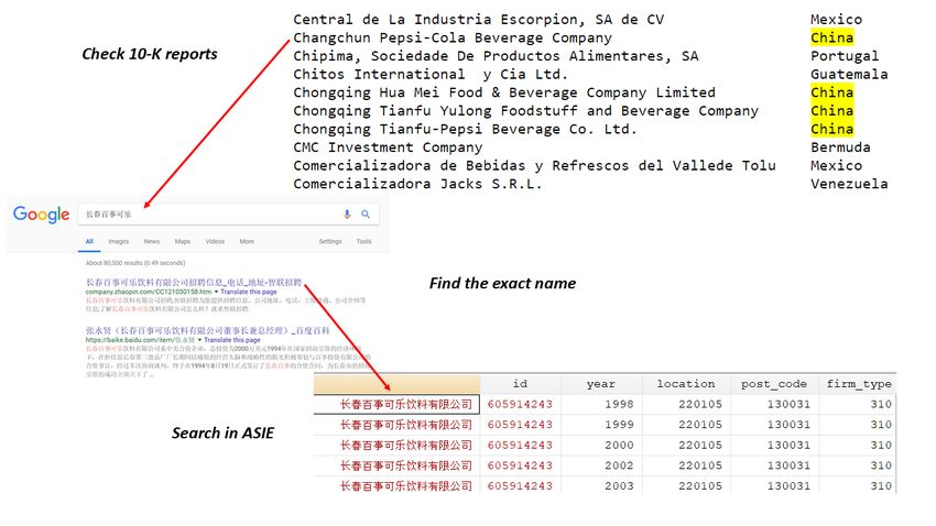
2.3. Matching U.S. public firms to their Chinese subsidiaries
Recent research in both economics and finance has exhibited increasing interest in ex-
ploiting the textual data of firms’ financial reports to garner information not presented in
financial statements.13 For example, Hoberg and Moon (2017) and Hoberg and Moon (Forth-
coming) use 10-K filings to determine companies’ exposure to off-shoring activities and relate
such measures to these public companies’ stock market performance. This paper expands
the existing approaches that utilize financial reports by extracting exact parent-subsidiary
information from the 10-K files. Relative to other potential data sources for identifying
14
parent-subsidiary linkages, the current study directly constructs the relationship based
on publicly accessible financial reports and can be combined with rich firm-level panel data
from both the U.S. and China.
The matching of U.S. public companies with their Chinese subsidiaries involves both au-
tomated textual search algorithms and hand-matching. I primarily use the annual 10-K files
from the Securities and Exchange Commission (SEC) database to construct these relation-
12
The data were recently used in studies such as Bombardini et al. (2017).
13
For example, Hoberg and Phillips (2010) and Hoberg and Phillips (2016) construct 10K-based product
similarity measures; Loughran and McDonald (2011) construct 10K-based measures of tones, and Bodnaruk
et al. (2015) construct a 10K-based measure of financial constraints.
14
Branstetter et al. (2006), Keller and Yeaple (2013), Bilir and Morales (2018) use the within-company
transaction records from confidential data of the U.S. Bureau of Economic Analysis (BEA); Jiang et al.
(2018) uses the Name List of Foreign and Domestic Joint Ventures in China from the China’s Ministry of
Commerce.
9ships. The 10-K files are annual U.S. public firm financial reports required by the SEC, and
they include not only standard financial statements, but also rich textual information about
the companies’ operations and outcomes. I first download all 10-K files from the SEC Edgar
database and then identify the U.S. firms that mention related keywords in their 10-K files
through text scraping. Specifically, I define the U.S. firms as related if their 10-K files include
the words “China” or “Chinese” plus “subsidiary,” “operation,” “facility,” “investment,” or
“venture” in the same sentence. I also randomly select about 50 financial reports to validate
my search. The validation results confirm the searching algorithm targets the companies
with various forms of operations in China.
Of these potential candidate firms, I manually examine the Exhibit 21 tables (list of
subsidiaries) in the 10-K files to extract the detailed names and locations of their Chinese
subsidiaries if they exist. When the Exhibit 21 tables are missing or do not contain any
Chinese subsidiary information, I also examine the main text of the 10-K files to search
for the related keywords and record the exact forms of these firms’ operations in China. A
large proportion of these firms report sales offices, representatives, or business partners in
China rather than manufacturing subsidiaries. I also supplement my list of subsidiaries from
10-Ks with an additional list of Chinese subsidiaries of U.S. companies from the ORBIS
database, which exclusively contains currently operating subsidiaries. I exclude from the
list the subsidiaries that were initiated after 2000. I demonstrate that the ORBIS data
adds 25 more U.S. public firms and 42 additional subsidiaries to my final matches, which
indicates my 10-K-based method of identifying subsidiaries of U.S. public firms captures a
major proportion of possible matches.
I then manually match these subsidiaries (both from 10-Ks and ORBIS) with the ASIE
data one by one. The names are often not precisely identical after translation into Chinese; I
therefore use keyword searches in multiple search engines to determine the names and infor-
mation of the subsidiaries. For each potential match, I also investigate the name, location,
industry, starting year, and ownership information to ensure the match is correct.15
Lastly, I restrict my focus to the subsidiaries from between 2000 and 2007 to eliminate
15
Figure A.1 shows my name-matching procedure using Pepsi Co. as an example.
10selection problems, because the entry and exit decisions of the subsidiaries could be correlated
with innovation shocks from the U.S. parents. I also restrict the parent companies of these
subsidiaries to the U.S. companies that exist (and are not acquired) between 2000 and 2007
in the Compustat data.
Of all 4,918 U.S. public companies that existed between 2000 and 2007, about 20% are
associated with China-related keywords, and I discover 224 U.S. public firms that include
subsidiary information that can be matched to the ASIE data. I examine the main text of
10-Ks of the other firms and determine that a substantial proportion of them have discussed
their sales office, representatives, or business partners in China when referring to the related
keywords. Therefore, I am unlikely to overlook a substantial number of U.S. public firms’
subsidiaries due to missing information in the 10-Ks. Including firms from the ORBIS data
and restricting them to subsidiaries starting before 2000 changes the numbers to 235 U.S.
public firms and 452 subsidiaries in China. Finally, matching with the patent data reduces
the number of public firms to 210 and the number of subsidiaries to 325 because some of
the U.S. public firms did not file any patents or were not matched to the patent database.
Because I could not distinguish between the two, I eliminate these firms from my final
match.16
As of year 2000, the largest MNC in the linkage is Motorola Solutions Inc., which em-
ployed over 13,000 people total and experienced sales of over 34 billion yuan (over 4 billion
U.S. dollars) in 2000. Notably, most of the matched MNCs are in high-tech industries, such
as electronics (Motorola, Flextronics, Emerson), machinery (United Technologies, General
Electric, Cummins), and chemistry (DuPont and Procter & Gamble).17
2.4. Measuring technology stocks
Measuring technology shocks is based on patent stocks of U.S. public firms. I utilize
the Harvard Patent Dataverse to compute the citation-weighted patent counts, and use the
crosswalk provided by Kogan et al. (2017) to match the patents with the Compustat public
firms.
16
Table A3 presents the matching rate for each step.
17
Table A4 presents the top 15 U.S. MNCs in size from the final match.
11The truncation problem presents a classic challenge of using the patent counts and cita-
tion counts (Hall et al. (2001)): when closer to the final year of the patent data, the patent
counts are downward-biased due to the absence of applied patents that have not yet been
granted, and the citation counts are also downward-biased because of the missing citations
from patents granted after the final year. I address the truncation problem by implement-
ing Hall et al. (2001) and Hall et al. (2005)’s quasi-structural approach that estimates the
empirical distribution function of both patent counts and citation counts for each of the six
technology categories and adjusts the counts in later years using the deflators based on the
estimation results.18
I apply the perpetual inventory method with a 15% depreciation rate, as suggested in
the previous literature,19 to construct the patent stock measures:
P
Kmt = (1 − η)KPmt−1 + Pmt .
In the equation above, m denotes U.S. MNCs and t denotes years varying from 1975 to
2010; K P is the cumulative patent stock, and Pmt is m’s citation-weighted patent counts in
the application year t. I primarily use citation-weighted patent stock to measure technology
levels of U.S. public firms because the weighting scheme accounts for the importance of each
patent.
I use parent company m’s three-year lagged patent stock as a proxy for the potential
technology transfers from m to its foreign subsidiary n:
sub
T ECHmnt = Log(Kmt−3 ).
After identifying the domestic firms that locate in the same county of the subsidiaries, I
measure local technology stocks as a weighted sum of the subsidiary-level technology stocks,
with the initial share of subsidiaries’ employment in each county as weights:
X wn0
T ECHctloc = log( Km(n)t−3 · ).
n∈Nc
Wc0
18
The detailed adjustment procedure is outlined in the appendix.
19
See, for example, Hall et al. (2005), Matray (2014). An alternative choice is to use a 10% depreciation rate
as in Keller (2002) and Peri (2005).
12In the equation above, Nc is the set of all matched subsidiaries in county c, Km(n)t−3 is n’s
parent company n(m)’s patent stock at year t − 3, wn0 is the initial employment of n, and
Wc0 is the total employment of firms in county c in the initial year. In other words, I use
the employment share of n in county c as weights to compute the aggregated county-level
technology stocks of MNCs. I use the time-invariant weights to avoid potential endogeneity
problems due to technology-induced changes in subsidiary sizes. The local technology stocks
measure serves as a proxy for the potential technology spillovers from the subsidiaries to the
domestic firms in the same county.
The measure of local technology stocks can be rationalized through a simple model in
which local technology diffusion is realized by the connections between workers in the multi-
nationals and local firms. I first assume each U.S. subsidiary n with size Ln is embedded with
technology level Tn from their parent company m. In each period, x percent of employees of
n have contact with any other workers in the local firms with equal probability.20 Assuming
the local economy is of size L, each worker in the local firm has an equal probability of x · LLn
having contact with the employees of n and of benefiting from the knowledge spillovers of
size Tn . The technology spillovers that originated from subsidiary n are therefore x · Tn ·LLn ,
and the overall local technology spillovers are x · n∈Nc TnL·Ln . By replacing the technology
P
level Tn with lagged citation-weighted patent stock Kmt−3 and size Ln with the initial level
of employment sn0 , the formula coincides with the construction of local technology stocks.
Figure 2 illustrates the geographic distribution of T ECH l oc in 2000. Many of the affected
counties are clustered around the four largest cities, namely, Beijing, Shanghai, Guangzhou,
and Shenzhen, as well as more developed provinces, such as Jiangsu, Zhejiang, and Guang-
dong. However, the influence of the MNC subsidiaries is also disseminated nationally: many
of the subsidiaries are located in the northeast, southwest, and central part of China, and
some of these subsidiaries are also linked to the most innovative U.S. parent companies.
I begin with this general measure that reflects the potential local technology spillovers on
all manufacturing firms in nearby counties, which facilitates an understanding of the overall
impact of the multinationals’ innovation activities on the local economy. Section 5 constructs
20
Alternatively, assume in each period that x percent of multinationals’ employees randomly flow from those
multinationals to the local firms.
13Figure 2: Geographic distribution of T ECH loc in 2000
Notes: This figure shows the geographic distribution of the measured technology spillover, which is the 3
year lagged log weighted sum of citation-weighted patent stock of the subsidiaries’ U.S. parent firms. The
subsidiaries are located in 121 counties out of 2280 in total. On average the matched subsidiaries account
for 7.3% of the total employment and 19.0% of the total output of the counties where they located.
industry-specific measures of local technology stocks based on subsidiaries’ industry codes
and technological relationships between the multinationals and local firms.
2.5. Productivity estimation
The primary outcome variables of the analysis include local firms’ value-added output
(va), revenue-based total factor productivity (tf pr), and labor productivity (lb). Because
the construction of value-added output and labor productivity is straightforward, this section
briefly introduces the construction of TFPR.
Directly measuring firms’ production efficiency (tf pq) based on the ASIE data is infeasible
due to the lack of exact input and output price data at the firm level. As such, I have instead
estimated the revenue-based total factor productivity (tf pr) and discussed the effects on tf pq
under specific assumptions.
I mainly apply Ackerberg et al. (2015) method (henceforth the ACF method) to mea-
14sure firm-level TFPR. First, I assume the following “value-added” Cobb-Douglas production
function:
yit = βk kit + βl lit + πit + it .
In this function, yit represents the value of the value-added output, kit represents capital,
and lit represents total employment. Two components constitute the residual term: the
persistent factor, πit , and the idiosyncratic factor, it , which consists of transitory shocks
and measurement errors. The value-added production function assumes gross output is
Leontief in the intermediate input mit ; therefore, the intermediate input is proportional to
the gross output.21
I estimate the production function based on the ACF two-stage method.22 In the first
stage, I estimate the output function using a 3-order polynomial of l, k and m, controlling
for a set of fixed effects and, most importantly, a set of multinationals’ technology stock
variables constructed in the previous sections, as suggested by Pavcnik (2002). In the second
step, I implement the generalized method of moments (GMM) estimator to recover the
coefficients for capital and labor at the same time. The estimated TFPR is therefore π̂it =
yit − β̂k kit − β̂l lit .
2.6. Summary statistics
Table 1 displays the summary statistics of the key variables in the analysis. Panel A
includes the sample of all matched subsidiaries of the U.S. public firms, and panel B includes
the sample of all local firms in the matched Chinese counties. Panel C indicates the distribu-
tion of the technology-shock measures. Comparing panel A with panel B demonstrates that
the matched subsidiaries are larger in size and more productive than local firms in nearby
geographic areas. The matched subsidiaries are, on average, 975% of the annual sales of the
domestic firms, 246% of the total employment of the domestic firms, and 200% of the TFP
of the domestic firms. The subsidiaries also pay 216% higher wages to their employees and
export much more than the local Chinese firms, on average. The differences persist after
21
The value-added production function assumption is discussed in, for example, Bruno (1978), Diewert
(1978), and Levinsohn and Petrin (2003).
22
the detailed estimation procedure is outlined in the appendix.
15Table 1: Summary statistics
Variables Mean Median Std. Dev. N
Panel A. Matched subsidiaries
Value added (millions RMB) 199.59 4.83 1125.30 1,957
Gross output (millions RMB) 673.03 165.56 3857.75 1,957
TFPR 2.41 2.85 2.14 1,957
Labor productivity 5.17 5.58 2.14 1,957
Employment 496.43 203.00 1045.79 1,957
Wage (thousands RMB) 48.07 37.75 36.05 1,957
Export value (millions RMB) 267.18 14.60 2250.20 1,957
Panel B. Local firms
Value added (millions RMB) 17.93 4.03 224.52 226,097
Gross output (millions RMB) 69.39 16.42 757.15 226,097
TFPR 1.42 1.65 1.78 226,097
Labor productivity 3.82 4.01 1.74 226,097
Employment 202.83 86.00 643.17 226,097
Wage (thousands RMB) 15.20 12.43 10.42 226,097
Export value (millions RMB) 4.49 0.00 166.36 226,097
State ownership (%) 21.80 226,097
Collective ownership (%) 19.40 226,097
Private ownership (%) 58.80 226,097
Panel C. Technology shocks
Parent-subsidiary tech. shocks 7.80 8.27 2.64 1,957
Local tech. shocks 2.85 3.16 3.47 226,097
Within-industry shocks 0.56 1.3 3.85 24,512
Shocks to upstream -2.18 -1.98 3.85 185,393
Shocks to downstream -2.15 -1.9 3.5 187,827
Tech.-distance based shocks 0.97 1.17 3.44 222,403
Notes: The table presents the summary statistics of key variables
in the main analysis, in which panel A presents the characteristics
of matched subsidiaries, panel B presents characteristics of local
firms in the matched counties, and panel C presents the distri-
bution of technology shock measures. The units are noted in the
parentheses, if necessary.
controlling for county, industry, and ownership fixed effects. These substantial differences
not only validate our matches of U.S. subsidiaries, but also indicate the subsidiaries may
induce sizable technology spillovers for local firms, as the subsidiaries are not only large in
size, but also technologically advantageous relative to local firms.
163. Specification and Identification Strategy
3.1. Specification
I estimated the effect of technology shocks exerted by parent companies on their foreign
subsidiaries (the intra-firm technology transfer effect) and the effect of local technology
shocks on domestic firms (the local technology spillover effect) using the following fixed
effect models, respectively:
Ynt = fn + ft + θsub T ECHnt
sub
+ Xnct + sub
nct ;
Yict = fi + ft + θloc T ECHctloc + loc
ict .
In these equations, n denotes matched subsidiaries, i denotes local Chinese firms, c denotes
counties, and t denotes years. Y refers to the outcome variables, and Xct refers to the control
variables. I include firm fixed effects to control for any time-invariant firm characteristics.
I also control for year fixed effects to capture any common shocks to all firms during the
year. The general year fixed effect is further divided into industry-year fixed effects to absorb
any industry-specific shocks, such as industry supply or demand shocks in each year, and
ownership-year fixed effects, which are intended to absorb any ownership-specific shocks,
such as the SOE reforms in the 2000s. The robust standard errors are clustered at the
parent company level in the parent-subsidiary technology transfer specification, and the
robust standard errors are clustered at the county level in the local technology spillovers
specification. The regressions are weighted using the initial employment of the firms for the
following reasons: First, the weighting scheme controls for the heteroskedasticity in the initial
firm size (Greenstone et al. (2010)); second, the estimated coefficients of the regression results
can be interpreted as “per capita” effects; third, the weighting scheme is also consistent with
the conceptual framework of knowledge transfer through worker connections or worker flows.
The coefficients of interest are θsub and θloc . θsub represents the estimated parent-subsidiary
technology transfer elasticity, and θloc represents the estimated local technology spillover
elasticity.
The OLS estimates could suffer from endogeneity problems, such that cov(T ECH sub , sub ) 6=
0 (patent stocks of multinationals correlate with unobserved shocks that affect subsidiaries’
17outcomes) or cov(T ECH loc , loc ) 6= 0 (multinationals’ technology stocks correlate with un-
observed shocks that affect local firms’ outcomes). First, as in the classic simultaneity prob-
lem (the “correlated effect” as in Manski (1993)), MNC headquarters, foreign subsidiaries,
or local Chinese firms could respond simultaneously to identical unobserved shocks. In the
parent-subsidiary technology transfer specification, a negative bias could be caused by CEO’s
limited attention23 ; that is, if CEOs occasionally allocate attention from foreign operations to
domestic research and development centers, the increase in innovation outcomes in the U.S.
will be associated with the contraction of foreign operations, thereby creating a negative bias
in the OLS estimates. In the local technology spillover specification, a bias could result from
unobserved supply or demand shocks. For example, an unobserved positive global supply
shock that enhances both local Chinese firms’ performance and multinationals’ innovation
outcomes would create a positive bias in the OLS estimates. Conversely, an unobserved shift
in tastes toward multinationals’ products (or high-quality products) in the global market
that also reduces the market demand for the Chinese products would produce a negative
bias in the OLS estimates.
The second source of bias relates to the sorting behaviors of the multinational sub-
sidiaries. Specifically, the innovation capacity of the multinationals may correlate with their
unobserved ability to select subsidiary locations, thereby resulting in bias in OLS estimates.
This type of bias could be either positive or negative: if multinationals prefer locations with
lower expected wages and input cost growth, and if more innovative multinationals are su-
perior in selecting the preferred locations for their subsidiaries, the bias would be negative;
conversely, if multinationals prefer locations with higher levels of human capital stocks and
faster market-demand growth, the bias would be positive.
To address potential endogeneity issues, I first restrict the sample of subsidiaries to
those initiated before 2000 so that the entry decisions are unlikely to be affected by the
multinational parents’ innovation activities during the sample period. I further introduce an
instrumental variable strategy based on the U.S.’s R&D tax credit policies in the following
section.
23
See, for example, Schoar (2002) and Seru (2014), for empirical evidence of CEO limited attention.
183.2. The U.S. R&D tax credit
The U.S. research and experimentation tax credit, or the R&D tax credit, consists of two
parts: the federal tax credit system and the state tax credit system. The federal R&D tax
credit was first introduced in the Economic Recovery Tax Act of 1981. The policy grants
a 25% tax credit for all qualified research and development expenses (QRE) defined by the
U.S. Internal Revenue Code (IRC).24 Since 1981, Congress had extended the R&D tax credit
policy multiple times, and made it permanent in 2015.
The introduction of the state R&D tax credit policies closely align with that of the
federal policy, and the state tax codes typically apply the same QRE definition as the
federal government. In 1982, Minnesota became the first state to introduce the state R&D
tax credit. As of 2007, 32 U.S. states have introduced some form of the R&D tax credit, and
Hawaii, Rhode Island, Nebraska, California, and Arizona have the highest effective credit
rate, ranging from 11% to 20%.
The effective state R&D tax credit rates commonly change over the course of years
due to policy adjustments.25 Figure 3 illustrates the changes in these tax credits from
1994 to 2001 (the duration of my analysis), and displays significant variation in state-level
R&D tax credit policy adjustments. Furthermore, the impact of the tax credits on firms’
research and development investment may also correspond with macroeconomic fluctuations
and other tax policy changes, such as interest rates and corporate income tax rates. To
adjust for these factors, I use the state-specific, R&D tax credit-induced user cost of research
and development capital (henceforth, user cost of R&D capital), constructed following Hall
(1992), Wilson (2009), and Bloom et al. (2013) in my instrumental variable construction.26
3.3. Instrumental variable construction
I construct the instrumental variable in four steps. First, I compute each firm’s patent
stock in each state in year 1997, which corresponds to the starting year of the three year
24
The three main components of eligible research expenses are: wages; supplies; contract research expenses,
as in the 2005 IRC section 41. Please see Audit Techniques Guide: Credit for Increasing Research Activities
for the detailed definition.
25
For example, Arizona changes its tax credit rate from 20% to 11% in year 2001.
26
The formula to construct the user cost of R&D capital is presented in the appendix.
19Figure 3: Changes of R&D Capital User Cost and Median Log Patent Stock
Notes: The figures show the geographic distribution of the changes of R&D capital user cost and
median log patent stock. The upper figure shows the change of R&D capital user cost from 1994
to 2001, and the lower figure shows the change of median firm-state log patent stock from 1997 to
2004, corresponding to the time period in our main analysis.
Change of R&D Capital User Cost
Change of Median Log Patent Stock
lagged measures of technology stocks. The patent stock share in each state is a proxy of
the geographic distribution of the firm’s innovation activities. Based on the state-specific
average user cost of R&D capital, I compute the firm-specific user cost of R&D capital as:
X
ρ̃it = wis ρhst ,
s∈S
20where ρhst is the user cost of R&D capital for the highest tier of R&D spending firms in state
s and year t, and wis is firm i’s share of citation-weighted patent stocks in state s and year
1997.
I further compute a cumulative R&D user cost (similar to my patent-stock construction)
as:
t
0
X
Zitsub = (1 − η)t −ti0 log(ρ̃¯it0 ),
t0 =ti0
where ti0 is the starting year of firm i, η = 15% is the depreciation rate of knowledge capital,
and ρ̃¯it0 is the average firm-level user cost of R&D capital from t0 − 3 to t0 . The coverage of
three years before the patent application year is to account for research durations.27
The firm-specific cumulative user cost of R&D capital is directly used as the instrument
for the technology transfers from the U.S. parents to their subsidiaries. The first-stage re-
gression specification in identifying the parent-subsidiary technology transfer effect is written
as:
sub
T ECHnt = fn + ft + λsub Zm(n)t−3
sub sub
+ νnt ,
where I control for subsidiary fixed effect fn and year fixed effect ft , with standard errors
clustered at the parent company level. λsub is the coefficient of interest, which represents the
elasticity of the parents’ patent stocks in response to the cumulative log R&D capital user
costs.
Next, I compute the weighted average of the user costs at the Chinese county level, based
on the initial size of the subsidiaries in China:
Z sub · wn0
P
n∈Nc
Zctloc = P m(n)t−3
0
,
n∈Nc wn
in which wn0 is the initial employment of subsidiary n, and Nc is the set of all matched
subsidiaries in c. The term can be interpreted as the average cumulative R&D user cost of
the parent companies of all foreign subsidiaries in the county.
The first-stage regression specification in identifying the local technology spillover effect
27
In the appendix, I show the cumulative R&D user cost construction is an approximation of a constant
elasticity relationship between patent counts and R&D user cost.
21is represented as:
loc
T ECHict = fi + ft + λloc Zct−3
loc loc
+ νict .
The first-stage regression would be conducted at the Chinese local firm level, where fj is
the firm fixed effects, and ft is the year fixed effects, which could be further replaced by
sector-year fixed effects and ownership-type-year fixed effects. As in the previous equation,
λloc is the coefficient of interest, representing the elasticity of local technology stocks of
multinationals in response to the average cumulative log R&D capital user cost changes.
Table 2: First-stage Regressions
First-stage regressions, 2000-2007
Dependent variables TECHŝub TECHl̂oc
(1) (2) (3) (4)
Z sub -2.316*** -2.272***
(0.640) (0.620)
Z loc -0.991*** -0.992***
(0.208) (0.188)
Local controls No Yes
Firm fixed effects Yes Yes Yes Yes
Year fixed effects No No Yes No
Sector-year fixed effects Yes Yes No Yes
Ownership-year fixed effects No No No Yes
Sample Subsidiaries Local firms
Observations 1,957 1,957 226,097 226,097
R-squared 0.982 0.982 0.9937 0.994
Notes: The table presents the first-stage regression results for the
parent-subsidiary technology transfer specification and the local
technology spillovers specification. Robust standard errors are clus-
tered at parent company levels in columns 1 and 2, and at county
levels in columns 3 and 4. ***, **, and * indicate significance at
the 1%, 5%, and 10% level.
Table 2 displays the first stage regressions. The results show the constructed instruments
exert negative effects on the corresponding multinational technology shocks, which are both
economically and statistically significant. The F-statistics of the first-stage regressions are
at least around 10, which is the lower bound of strong instruments, as suggested by Stock
and Yogo (2002).28
28
In the appendix, I discuss how the identification strategy of using the cumulative user cost of R&D capital
might fulfill the criteria of the exclusion and inclusion restrictions in detail.
224. Technology Transfers and Local Technology Spillovers
4.1. Parent-subsidiary technology transfers
I examine the relationship between parent companies’ innovation and their subsidiaries’
performance. This step serves as a validation assessment because the existence of the parent-
subsidiary technology transfers is necessary for the multinationals’ local technology spillover
effect. Additionally, the question concerning whether technology advances of the parent com-
panies are transmitted to their foreign subsidiaries is worth investigating in itself. Previous
studies have documented substantial technology transfers within multinationals (Branstet-
ter et al. (2006)). A parallel strand of literature has established that productivity shocks of
parent firms could be transmitted to their foreign subsidiaries (for example, Boehm et al.
(2019), Bilir and Morales (2018)). However, few studies have yet investigated whether tech-
nological improvements in parent companies also generate productivity gains in their foreign
subsidiaries.
I begin by studying how the matched subsidiaries’ log value-added output, TFPR, la-
bor productivity, and markups are affected by their parent companies’ three year lagged
citation-weighted patent stocks (T ECH sub ). I control for firm fixed effects that eliminate
any time-invariant subsidiary characteristics and industry-year fixed effects that absorb in-
dustry specific shocks in each year. I further include the mean sales, TFPR, and markups
level of the local firms in the same sector and county of each matched subsidiary in the re-
gressions to control for the local economic conditions. Last, as previously discussed, I weight
each firm by its initial employment level and cluster the robust standard errors at the parent
company level.
Table 3 presents the regression results. Column 1 suggests a 10% increase in the par-
ents’ lagged patent stocks is associated with a 2.8% increase in the subsidiaries’ value-added
outputs. As indicated in Column 2, controlling for the local economic conditions did not
eliminate the positive correlations between the parents’ lagged patent stocks and the sub-
sidiaries’ value-added outputs. The IV estimate using the cumulative user costs of research
and development capital as instruments in Column 3 indicates a 10% increase in the parents’
lagged patent stocks causally increases the value-added outputs of the subsidiaries by 5.8%.
23In Column 3 relative to Column 2, the IV estimate is approximately double the OLS esti-
mate, which may either be due to attenuation bias (because the standard error also becomes
larger) or unobserved factors, such as CEO attention, as discussed previously. Column 4
shows the TFPR is also positively correlated with the parents’ technology shocks, but the
OLS estimate presents negative bias (compared with Column 5). Columns 5 and 6 suggest
a 10% increase in the parents’ lagged patent stocks causally increases the revenue-based
productivity measures, including TFPR and labor productivity, by about 3.6% to 3.8%
respectively.
Table 3: Effects of the parent-subsidiary technology shocks
Parent-subsidiary technology transfers
Dependent variables va va va tfpr tfpr lp
(1) (2) (3) (4) (5) (6)
Models OLS OLS IV OLS IV IV
T ECH sub 0.279*** 0.307*** 0.579*** 0.213** 0.380** 0.362**
(0.0929) (0.104) (0.198) (0.0888) (0.163) (0.171)
Local controls No Yes Yes Yes Yes Yes
Industry-year FE Yes Yes Yes Yes Yes Yes
First-stage F-stats 15.594 15.594 15.594
Observations 1957 1957 1957 1957 1957 1957
R-squared 0.767 0.769 0.767 0.692 0.691 0.682
Notes: The table presents the regression results of the effects the parent-
subsidiary technology shocks. Regressions are weighted using the initial
employment of the firms. Robust standard errors are clustered at the parent
company level. ***, **, and * indicate significance at the 1%, 5%, and 10%
level.
I also investigate how the other firm-level outcomes of the subsidiaries respond to the
parent companies’ technology stocks.29 I find subsidiaries’ average wage and return on assets
respond to the technology shocks at 10% significance level.
4.2. Local technology spillovers
The results presented in the previous subsection confirm that the subsidiaries of the U.S.
multinationals benefit from technological advances of their parent firms. The next question
is to ask whether the local firms in China also benefit from the technological improvements of
the multinationals in the local areas. This subsection addresses this question by examining
29
See Table A8.
24how the local firms’ log value-added output, TFPR, and labor productivity, are affected by
the multinationals’ local technology shocks (T ECH l oc), which is measured in terms of the
log weighted sum of lagged patent stocks. I control for firm fixed effects and year fixed
effects (or industry-year and ownership-year fixed effects) in the regressions, and weight the
regressions in terms of the initial employment of firms. Robust standard errors are clustered
at the county level.
Table 4: Effects of the local technology shocks
Local technology spillovers
Dependent variables va va va tfpr tfpr lp
(1) (2) (3) (4) (5) (6)
Models OLS OLS IV OLS IV IV
T ECH loc 0.214** 0.201* 0.331* 0.169** 0.249** 0.242**
(0.104) (0.108) (0.181) (0.0835) (0.116) (0.117)
Firm FE Yes Yes Yes Yes Yes Yes
Year FE Yes No No No No No
Industry-year FE No Yes Yes Yes Yes Yes
Ownership-year FE No Yes Yes Yes Yes Yes
First-stage F-stats 27.866 27.866 27.866
Observations 226097 226097 226097 226097 226097 226097
R-squared 0.707 0.719 0.719 0.615 0.615 0.606
Notes: The table presents the regression results of the effects the local
technology shocks. Regressions are weighted using the initial employ-
ment of the firms. Robust standard errors are clustered at the county
level. ***, **, and * indicate significance at the 1%, 5%, and 10% level.
Table 4 presents the regression results. Column 1 shows a 10% increase in the local
technology stocks is associated with a 2.1% increase in the local firms’ value-added outputs,
and the magnitude changes to 2.0% after controlling for industry-year and ownership-year
fixed effects rather than year fixed effects in Column 2. Column 3 shows a 10% increase in
the local technology stocks causally leads to a 3.3% increase in the value-added outputs of
the local firms at 10% significance level. Similar to the previous results, the IV estimate is
approximately twice as large as the OLS estimate, suggesting a negative bias due to either
attenuation bias, or the global shocks as previously discussed. Column 4 shows the TFPR is
also positively correlated with the local technology stocks, but the OLS estimate is negatively
biased (when compared with Column 5). As shown in Columns 5 and 6, a 10% increase in
the local technology stocks also causally increases local firms’ revenue-based productivity
measures by 2.4% to 2.5%.
25I also investigate the effect of the local technology stocks on the other outcomes of local
firms,30 and find the local firms’ average wage and intangible assets are responding positively
to the local technology stocks at 10% significance level. Furthermore, the local technology
shocks also improve the survival rate of the more productive firms.31 .
4.3. Magnitudes
I discuss the implied magnitudes of the identified effects in the baseline regressions in de-
tail. First, one within-firm standard deviation in the parent-subsidiary technology transfers
(0.372) leads to a 21.5% increase in the subsidiaries’ value-added outputs, a 14.1% increase
in the subsidiaries’ TFPR, and a 13.5% increase in the subsidiaries’ labor productivity. The
one-standard-deviation effect of the parent-subsidiary technology transfers on TFPR explains
about 9.0% of the within-firm TFPR variations in the matched subsidiaries.
Meanwhile, one within-firm standard deviation in the local technology spillovers from
the U.S. multinationals (0.221) leads to a 7.3% increase in the local firms’ value-added
outputs, a 5.5% increase in the local firms’ TFPR, and a 5.3% increase in the local firms’
labor productivity. The one-standard-deviation effect of the local technology spillovers on
TFPR explains approximately 4.87% of the within-firm TFPR variations in the matched
subsidiaries. Additionally, the intra-firm effect of technology shocks is more substantial
than the inter-firm one. The difference could be driven by firm boundaries that impede the
transfer of technology from multinationals to domestic firms.
4.4. Robustness Checks
This section provides a list of robustness checks to address various potential concerns
regarding the baseline results.
In the primary analysis, I have made one seemingly arbitrary assumption: I presume
the duration of international technology diffusion through multinationals is three years. I
examine alternative choices regarding the duration of technology spillovers.32 I find the
parent-subsidiary technology transfer effects are significant at the 5% level for lagged years
30
See Table A9.
31
See Table A10.
32
The results are shown in Figure A.6
26You can also read