An Integrated London Journey Planner - Department of Computing
←
→
Page content transcription
If your browser does not render page correctly, please read the page content below
Imperial College London

             Department of Computing

An Integrated London Journey
           Planner

                                                     Supervisors:
                                           Dr. Alessandra Russo
   Author:                                    Dr. Luke Dickens
   Ryszard T. Kaleta
                                                   Second Marker:
                                               Dr. Francesca Toni

                             19 June 2012

Submitted in part fulfilment of the requirements for the degree of Master of
         Engineering in Computing of Imperial College London
Abstract
Urban cycling is becoming increasingly popular. For many commuters and
tourists alike it is the cheaper and more pleasant alternative to traditional
modes of public transport. Urban cycling is supported by many cities world-
wide through introduction of cycling lanes and, more importantly to those who
do not own a pair of wheels themselves, also the creation of bicycle sharing
schemes.
City public transportation networks are not easy to navigate. This is why most
provide on-line journey planners that allow users to search for a desired mix
of transport links to reach destination. We believe that such journey planners
should also incorporate the bicycle sharing schemes. However, to build an effec-
tive journey planner one has to know the future arrival times of various modes
of transport such that waiting time whilst connecting is minimised.
The latter is a non-trivial task when it comes to bicycle sharing schemes because
there is no schedule of bicycle arrivals at various docking stations. This makes it
hard to plan cycling journeys that are to occur in the future and is the reason no
journey planner built thus far has fully catered for the needs of urban cyclists.
We aim to change all this by designing and implementing a journey planner
for London, UK that integrates a bicycle sharing scheme with other modes
of public transport whilst minimizing wait times at docking stations through
bicycle availability prediction.
Acknowledgements
I am grateful to Dr. Alessandra Russo and Dr. Luke Dickens for their continuous
support and guidance throughout the course of this project.
Above all, I would like to thank my parents and closest family - without them
I would not have been able to make it this far.
Contents

1 Introduction                                                                                                              3

2 Background                                                                                                                7
  2.1 Terminology . . . . . . . . . . . . . . . .                  .   .   .   .   .   .   .   .   .   .   .   .   .   .    7
  2.2 Bicycle Sharing Systems . . . . . . . . .                    .   .   .   .   .   .   .   .   .   .   .   .   .   .    7
  2.3 Transport for London . . . . . . . . . .                     .   .   .   .   .   .   .   .   .   .   .   .   .   .    8
  2.4 Journey Planning Data Sets . . . . . . .                     .   .   .   .   .   .   .   .   .   .   .   .   .   .   10
      2.4.1 Past cycle journeys . . . . . . . .                    .   .   .   .   .   .   .   .   .   .   .   .   .   .   10
      2.4.2 Live bicycle availability . . . . .                    .   .   .   .   .   .   .   .   .   .   .   .   .   .   10
  2.5 Probability Theory . . . . . . . . . . . .                   .   .   .   .   .   .   .   .   .   .   .   .   .   .   13
      2.5.1 The Basics . . . . . . . . . . . .                     .   .   .   .   .   .   .   .   .   .   .   .   .   .   13
      2.5.2 Density Models . . . . . . . . . .                     .   .   .   .   .   .   .   .   .   .   .   .   .   .   14
      2.5.3 Density Estimation . . . . . . . .                     .   .   .   .   .   .   .   .   .   .   .   .   .   .   15
      2.5.4 Maximum Likelihood Estimation                          .   .   .   .   .   .   .   .   .   .   .   .   .   .   16
  2.6 Graph Theory . . . . . . . . . . . . . . .                   .   .   .   .   .   .   .   .   .   .   .   .   .   .   17
      2.6.1 The Basics . . . . . . . . . . . .                     .   .   .   .   .   .   .   .   .   .   .   .   .   .   17
      2.6.2 Path finding . . . . . . . . . . . .                   .   .   .   .   .   .   .   .   .   .   .   .   .   .   17

3 System Architecture                                                                                                      20

4 Predicting Bicycle Availability                                                                                          23
  4.1 Model Definition . . . . . . . . . . . . . . . . .                           .   .   .   .   .   .   .   .   .   .   25
  4.2 Parameterizing the Model . . . . . . . . . . . .                             .   .   .   .   .   .   .   .   .   .   31
  4.3 Making Predictions . . . . . . . . . . . . . . . .                           .   .   .   .   .   .   .   .   .   .   32
      4.3.1 Using Cumulative Distribution Function                                 .   .   .   .   .   .   .   .   .   .   33
      4.3.2 By Sampling the Density Estimator . .                                  .   .   .   .   .   .   .   .   .   .   35

5 Routing                                                                                                                  41
  5.1 Graphs . . . . . . . . . . . .   .   .   .   .   .   .   .   .   .   .   .   .   .   .   .   .   .   .   .   .   .   42
  5.2 Modified astar path . . .        .   .   .   .   .   .   .   .   .   .   .   .   .   .   .   .   .   .   .   .   .   42
  5.3 Cost Models . . . . . . . . .    .   .   .   .   .   .   .   .   .   .   .   .   .   .   .   .   .   .   .   .   .   46
  5.4 Complete Journey Planning        .   .   .   .   .   .   .   .   .   .   .   .   .   .   .   .   .   .   .   .   .   52
  5.5 Pathmax Optimisation . . .       .   .   .   .   .   .   .   .   .   .   .   .   .   .   .   .   .   .   .   .   .   54

                                           2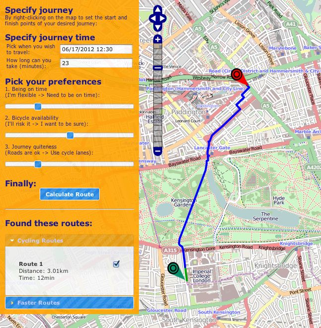
CONTENTS                                                                                                   3

6 Results and Evaluation                                                                                  57
  6.1 Bicycle Availability Model Performance      .   .   .   .   .   .   .   .   .   .   .   .   .   .   57
      6.1.1 Functional Performance . . . . .      .   .   .   .   .   .   .   .   .   .   .   .   .   .   57
      6.1.2 Non-Functional Performance . .        .   .   .   .   .   .   .   .   .   .   .   .   .   .   61
  6.2 Routing Algorithm Performance . . . .       .   .   .   .   .   .   .   .   .   .   .   .   .   .   67
      6.2.1 Functional Performance . . . . .      .   .   .   .   .   .   .   .   .   .   .   .   .   .   67
      6.2.2 Non-Functional Performance . .        .   .   .   .   .   .   .   .   .   .   .   .   .   .   68

7 Conclusions and Future Work                                                73
  7.1 Conclusion . . . . . . . . . . . . . . . . . . . . . . . . . . . . . . 73
  7.2 Improving Bicycle Availability Predictions . . . . . . . . . . . . . 74
  7.3 Improving Router . . . . . . . . . . . . . . . . . . . . . . . . . . . 75

A Journey Planner - In Action                                                                             77
Chapter 1
Introduction
Bicycle sharing systems are being introduced as the latest mode of public trans-
port all over the world (see section 2.2). The providers are driven by their
positive environmental impact to increase their popularity. The cyclists often
see these systems as a cheap and cheerful alternative to more traditional modes
of urban transport. Apart from introducing the systems themselves, the city
planners attempt to make their streets more bicycle-friendly. Most journey plan-
ning software allows the user to set a number of parameters before the route is
calculated, such that most desirable journey path can be found.
The amount of time an urban journey maker spends waiting whilst travelling on
public transport has a significant influence on their choice of transport and the
willingness to use it again. The more a passenger has to wait throughout their
journey, the less reliable the transport mode in question will seem. Journey
planners often consider current traffic and network conditions in their attempts
to find routes that are most desirable to the user yet avoid any ongoing delays.
This works well with modes of public transport that run according to a timetable
as alternative routes that avoid these problems can be easily found.
The vast majority of journey planners that are capable of incorporating cycling
into their routes assume the user owns a bicycle. Finding a cycling route is
then relatively easy as all we have to do is to take into account users’ prefer-
ences and find a path that satisfies them. This is done very successfully by a
number of free route planning solutions. Apart from turn-by-turn navigation,
cyclestreets.net [12] is able to provide a very impressive feedback on the pro-
posed cycling journey, including the number of burnt calories, CO2 avoided and
even the number of traffic lights and crossings that are passed on the way. A
number of OpenTripPlanner implementations [31] provide a similar service for
a number of cities around the world. Created from data gathered by the cyclists
themselves, they have the potential of containing information not found in other
cycling route planners, such as picturesqueness.
45
However, trying to include cycling into routes, when no assumption about bi-
cycle ownership can be made, is more difficult. This is because, while we are
keen to utilise the bicycle sharing systems, these have a limit on the number of
bicycles that are available at docking stations. The journey planning software
is unable to guarantee that the user will be able to start and finish their cycling
journey at the elected docking stations, since the docking stations of interest
may either be out of bicycles or have no free parking space left. This is partic-
ularly problematic if the bicycle sharing system charges their users for bicycle
hire - then, any delay that occurs because of inability to complete the cycling
journey as planned by the routing software is not only putting the user off using
that journey planning software and the bicycle sharing scheme again, but is now
also costly.
The problem is tackled by both the bicycle sharing systems’ providers as well
as the cycling journey planners. Transport for London, who own a large bicy-
cle sharing system in London, UK (called BCH and described in section 2.3),
provide the following guidelines when problems with picking up or dropping off
bicycles occur:
• if there are no bicycles at the docking station, the passenger can use the
docking station’s map to locate other docking stations nearby. There is
no guarantee there will be a bicycle available at those stations
• if the docking station is full, the passenger can get up to 15 minutes extra
time to cycle to another station before extra charges for late bicycle return
start to apply. As above, there is no guarantee that there will be a parking
space at the nearby stations
Often, this is not a good enough solution [24]. That is why we have seen a
number of mobile phone applications being developed that can locate the nearest
docking station and provide the latest available information on the number of
working bicycles and free parking spaces at that station. However, with this
solution the task of planning the journey is left to the user.
The most sophisticated solution to the problem is provided by journey planning
software that bases its suggested cycle routes around the use of bicycle sharing
schemes, but additionally considers the latest bicycle availability at all active
docking stations. If a docking station is currently out of working bicycles or all
of its docks are in use, the software seeks an alternative route that uses other
docking stations. Transport for London is the best example of such a journey
planner the author was able to find and we examine it in more detail in section
2.3.
All of the above routing software misses one important point - a user is rarely
able to begin their cycling journey the very moment they ask for a route to be
found. Normally, some time will pass between journey planning and the time
the user arrives at a docking station to start their journey. As such, using live
data on bicycle and parking space availabilities is not helpful as the state of the
world is likely to change between now and journey start time. From the time6 CHAPTER 1. INTRODUCTION
of planning the journey to actually reaching one of the docking stations the
bicycles that were available when we planned our journey might have by now
been taken away by other members of the public. The time a bicycle will be
returned to this station such that we can continue on our journey is unknown.
This is not the case for more traditional modes of public transport such as a
train or a bus, where a timetable of arrivals exits.
The only true way of improving the reliability of journey planning software that
includes cycle path routing based on bicycle sharing systems is to predict bicycle
availability at journey origin/destination docking stations at the time the user
is set to reach the docking station in question.
With this project, we aim to:
1. collect data on past BCH cycle journeys and current bicycle availability
across all BCH stations
2. devise a model capable of predicting future availability of bicycles at
BCH’s docking stations based on above historical evidence
3. devise a route planner that will combine walking, cycling and the London
Underground network to create a route that is most desirable to the user.
It should be capable of calculating routes based on distance, time and
route busyness
4. allow the user the control over the setting of those preferences such that
they are able to define what the most desirable route would be (mention
achieving this (maths wise) in cost models functions, and UI-functionality
wise when evaluating user experience)
5. incorporate the bicycle availability prediction model into said route plan-
ner in the aim of creating a more accurate and satisfying journey planning
experience
The end-product is an implementation of a journey planner capable of finding
routes combining walking, cycling and travel on the London Underground across
Greater London area. The journey planner tries to find a cycling route and when
this is not possible given user-defined preferences, a mix of walking, cycling and
London Underground routes is suggested as well. Our journey planner makes
no assumption of bicycle ownership and instead utilises a large bicycle sharing
scheme that exists in the city centre. It goes further than all other routing
software has ever gone before by attempting to predict future bicycle availability
within this system using density estimation techniques, such that the users feel
cycling can be a reliable mode of public transport. The journey planner interacts
with the users via map-based web interface that allows the users to specify their
most desirable journey across a number of parameters.
Whilst working on this project, we have also been able to contribute to Net-
workX, a Python language software package for the creation, manipulation,
and study of the structure, dynamics, and functions of complex networks. We7 have extended the functionality of NetworkX’s astar path to finding short- est paths in directed and undirected multigraphs, where only simple graphs were handled before [22]. The report is structured to describe our approach to each of the above aims in turn. Thus in Chapter 2 we describe the data we will use in developing bicycle availability models, themselves described in Chapter 4. In Chapter 5 we describe our routing methods that combine user’s preferences as to the desired journey with the predicted bicycle availabilities at docking stations. Our journey planner is built as a number of components whose design is briefly described in Chapter 3. Chapter 6 shows our results and asses the suitability of our methods. To see the journey planner in action, investigate figures in Appendix A.
Chapter 2

Background

2.1     Terminology

The following definitions will be used frequently throughout this report. We
clarify their indented meaning below:
   • BCH is an acronym we will use when referring to Barclays Cycle Hire
     scheme
   • Bicycles refers to bicycles that are part of the BCH
   • Docking station refers to the London-wide BCH terminals where bicycles
     can be parked and picked up form
   • Bicycle dropoff refers to the act of arriving at a docking station that is
     part of the BCH and parking the bicycle at an available dock
   • Bicycle pickup refers to the act of departing from a docking station that
     is part of the BCH by taking an available and functional bicycle out of its
     dock and cycling away

2.2     Bicycle Sharing Systems

Bicycle sharing system is a service that provides affordable access to bicycles to
individuals who do not own any themselves. Run mainly by local government
agencies, the systems are an alternative to motorized public transport on short-
distance trips. The authorities hope the systems will reduce traffic congestion,
noise and air pollution. As of 2011, around 300 such schemes were operating
worldwide [3]. Examples of successful implementation are manifold:

                                        8
2.3. TRANSPORT FOR LONDON 9
• Dublinbikes, setup in September 2009, reached 1 million uses in less than
a year
• Cyclocity programs, launched by JCDecaux, spread out of France into
Brisbane, Australia and Vienna, Austria
• New York City, USA plans to introduce its own Citibike system in July
2012. With 10,000 bicycles available from 600 stations spread throughout
the city, this will be the largest system of its kind in North America
Operating the bicycle sharing schemes can be very profitable too - Bixi [6],
a system developed by Public Bike System Company in Montreal, Canada,
recorded net income of CAD1.5 million in the financial year 2011 [33]. Since
most systems charge passengers on a per-trip basis, the providers are interested
in increasing the popularity of their bicycle networks.
2.3 Transport for London
Transport for London (TfL) is the local government body responsible for most
aspects of the transport system in Greater London. We are interested in TfL
for two reasons:
1. they own and operate BCH, described next, on which we shall use for the
cycling parts of the routes calculated by our journey planner
2. they provide data that we can use to build bicycle availability models.
This data, described in sections 2.4.1 and 2.4.2, is provided free of charge
and available to anyone who registers in TfL’s Developer’ Area [16].
Barclays Cycle Hire
BCH is a bicycle sharing system owned by Transport for London (TfL) that was
launched on 30 July 2010. Available 24 hours a day, this self-service operates
8,000 bicycles across 570 docking stations spread around 65 km2 of central
London. By March 2012, the system has registered 10 million ’hires’, making it
one of the most successful in the world [2]. This also means we will have access
to a substantial amount of historical data on which to build our availability
model.
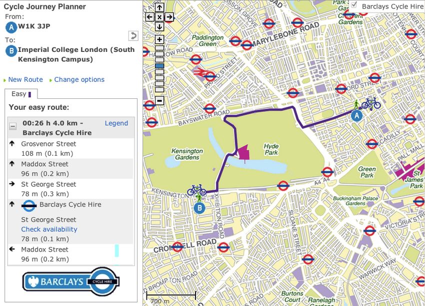
TfL already provides a cycle journey planner that incorporates BCH. Figure 2.1
shows the cycling journey planner following a request to calculate an exemplary
cycling journey across central London. The start and finish points are entered
manually by the user and we found that our home postcode was not recognised.
The route is calculated by finding BCH docking stations nearest to user-defined
start and finish locations. The route is then formed of three parts:10 CHAPTER 2. BACKGROUND
Figure 2.1: TfL’s Cycle Journey Planner[17]2.4. JOURNEY PLANNING DATA SETS 11
1. using the user-defined start location and the location of starting docking
station, the start-walk part of route is found. This helps the passenger
reach the nearest docking station
2. using the locations of starting and finishing docking stations, as well as
preferences for route busyness (set in options), the cycling part of resulting
route is found
3. finally, using the user-defined finish location and the location of the fin-
ishing docking station, the finish-walk part of the route is found
We can see in Figure 2.1 that the user can check live availability of a docking
station to check if bicycles are available. This is an availability check made at
the time the planner is used and no attempt is made to estimate the future
availability.
2.4 Journey Planning Data Sets
In this section we describe the data that we were able to and needed to obtain
as part of this project. We first describe the data we will need to build our
model of bicycle availability. We then briefly mention other data that is needed
to build our journey planner.
2.4.1 Past cycle journeys
We have obtained access to data listing all BCH journeys made from 30 July
2010 to 31 May 2011 [18]. Each journey record lists:
• bike ID
• journey start date and time
• start docking station
• end date and time
• end docking station
Methods described in sections 4.2 and 4.3 will use this data to estimate the
number of pickups and dropoffs for each docking station at different time points
of the day.
2.4.2 Live bicycle availability
We have also obtained access data listing the current status of every docking
station. Unlike the past cycle journeys data described above, this is a live feed
that comes directly from Serco Group’s database and is updated in three-minute12 CHAPTER 2. BACKGROUND
intervals, 24 hours a day, seven days a week [19]. Serco Group are the service
providers of BCH. Each update includes the following information on every
operation docking station:
• update time stamp
• name, location and co-ordinates
• availability for usage
• total number of bicycles available at a docking station
• number of docking points available at a docking station, excluding any
defective bike docks
• total number of docking points available at a docking station
Methods described in sections 4.2 and 4.3 will use this data to improve the
estimated number of pickups and dropoffs for each docking station at different
time points of the day, as calculated using past cycling journeys data described
above.
London Underground Data
Our journey planner will be capable of mixing journeys on the London Under-
ground into the routes it suggests to the user. For this, we need the following
information on every London Underground station:
• station name
• station co-ordinates
We would also like to know how the stations are connected, such that we can
find paths through the underground network. This means that for any two
connected London Underground stations we would like to know:
• the London Underground lines that connect these stations
• the distance travelled by the underground train between these stations
and the time this takes.
TfL does not provide a straight-forward access to above data. We have found
alternative sources [26][27][11]. Later we find that the data is not always 100%
accurate. Though we consider the accuracy good enough for a prototype appli-
cation, we note in Chapter 3 that our journey planner has been designed with
future improvements in mind - the underlying data can be easily swapped inside
our database for a more accurate set without any code changes.2.4. JOURNEY PLANNING DATA SETS 13
Greater London data
Finally, we need a data set from which a model of Greater London can be built.
We need such model so that we can apply the techniques described in chapter 5
for finding street-level paths for walking and cycling. The data has to comprise a
list of nodes (street level feature points such as junction) and edges (representing
connections between pairs of nodes, such as a footpath, road or a bridge). An
introduction to graph theory is provided in section 2.6. For now, we note that
for this data we turned to OpenStreetMap - a collaborative project to create a
free editable map of the world.
There are several reasons explaining our choice:
• our mapping needs require access to underlying data - the information,
listed below, about every street, path and other street-level link that forms
a network representing Greater London. If we were to collect data from
Google Maps, for example, we would be creating derived work. The data
Google uses in its maps service is either its own or licensed from mapping
companies (for example NAVTEQ and Tele Atlas) or national mapping
agencies, who made significant financial investment to obtain it and are
understandably protective of their copyright. In practice, if our jour-
ney planner used the Google Maps API, we could be subject to licensing
fees and contractual restrictions of these map providers. Use of Open-
StreetMap for our purposes is completely free
• there exists a number of usage limits that apply to the Google Maps API
• we find that OpenStreetMap provides more information for built-up areas
than Google Maps - house numbers are an example. There also exist a
number of layers that can be applied on top of the underlying map tiles
that show additional information, such as cycling routes or more points of
interest
Of course, we are only interested in the area of Greater London. Having obtained
an extract from OpenStreetMap that covers the city [10], we find it contains
the following information:
• co-ordinates of nodes
• for every edge:
– source and target nodes
– edge length and geometry (an edge does not have to be a straight
line)
– car accessibility, which also tells us what type of road this edge is
– bicycle accessibility, which also tells us how safe the edge is for cycling
– foot accessibility14 CHAPTER 2. BACKGROUND
The accessibility information will help us calculate routes that suite our journey
planner users’ route busyness preference.
2.5 Probability Theory
Our approach to bicycle availability prediction will rely heavily on probability
theory. Below we introduce the basics concepts that are required for under-
standing the topics discussed in later parts of this section.
2.5.1 The Basics
A random variable is a mapping from the sample space S to the real numbers,
such that if X is a random variable, X : S → R. Each element of the sample
space s ∈ S is assigned by X a numerical value X(s).
Probability distribution P is a function that describes the probability of X
taking certain values in R.
For a discrete random variable it holds that:
X
p(x) = P (X = x) = 1, ∀s ∈ S (2.1)
s
p(x) is then called the probability mass function and it gives us the probability
that a discrete random variable is exactly equal to some value [20].
The cumulative distribution function of random variable X tells us the proba-
bility that X takes a value less than or equal to x:
F (x) = P (X ≤ x), ∀x ∈ R
We can express the cumulative distribution function of a discrete random vari-
able in terms of its probability mass function:
k
X
F (xk ) = p(xi ) (2.2)
i=1
Similarily
k−1
X
P (X < xk ) = p(xi ) (2.3)
i=12.5. PROBABILITY THEORY 15
2.5.2 Density Models
Chapter 4 describes bicycle availability models. These models need to estimate
the number of bicycle pickups and dropoffs that occur at every bicycle docking
station at different times of the day. We can think of these numbers as discrete
random variables. They do this by estimating unobservable probability mass
functions p(X) that underlay these pickup/dropoff numbers. These models
of the true distributions of random variables are otherwise known as density
estimators or density models.
Density models can be parametric or non-parametric. The parametric density
models are assumed to be of particular form that is characterised by a set of
adjustable parameters θ, where θ ∈ R. In section 2.5.4 we introduce a method
for calculating these parameters. First, however, we introduce two parametric
forms of density models that will prove essential in our attempts to predict
bicycle availability at docking stations.
Binomial Distribution
Binomial distribution is a discrete probability distribution defined as
N
Pp (k|N ) = pk (1 − p)N −k (2.4)
k
Since the above definition involves the combination
N N!
= (2.5)
k k!(N − k)!
the binomial distribution can be thought of as describing the probabilities of
obtaining k successes on N trials. In our case the k can be thought of as the
number of dropoffs or pickups per some time interval in a day and N as the
number of days for which we have sample data.
Poisson Distribution
For reasons listed in section 4.1 we are mainly interested in the Poisson distri-
bution. Poisson distribution is another example of a parametric discrete prob-
ability distribution. It builds on the binomial distribution mentioned above to
describe the probability of the number of events that are likely to occur within
a fixed period of time. It is defined as the binomial distribution in the limiting
case where N → ∞, with p in (2.4) as the probability of a success.
If we set λ = N p, where λ can intuitively be thought of as the expected number
of occurrences of an event in some time interval i, equation (2.4) can be rewritten
as
N! λ λ
Pλ/N (k|N ) = ( )k (1 − )N −k (2.6)
k!(N − k)! N N16 CHAPTER 2. BACKGROUND
Considering the mentioned limit, equation (2.6) becomes
Pλ (k) = lim Pp (k|N )
N →∞
k
N! λ λ λ
= lim ( )(1 − )N (1 − )−k
N →∞ N k (N − k)! k! N N
N (N − 1)...(N − k + 1) λk
λ λ
= lim ( )(1 − )N (1 − )−k
N →∞ Nk k! N N
λk −λ
= (1)( )(e )(1)
k!
λk e−λ
= (2.7)
k!
Formally, λ is a positive real number such that
λ = E(X) = var(X) (2.8)
2.5.3 Density Estimation
Density estimation helps us define the set of parameters θ that characterises a
density model, such as a Poisson distribution, given observed data, such as that
discussed in sections 2.4.1 and 2.4.2. Because we consider the observed data
as having been drawn from the true distribution that we are trying to describe
with our density model, we can make the assumption that such model inferred
from such data is a good representation of this true distribution. In this context,
the observed data can be referred to as the sample data.
Formally, density estimation is the problem of modelling a true, unobservable
probability density (for continuous variables) or mass (for discrete variables)
function p(X) of a random variable X given a finite set of observations {xi }N
i=1
drawn from that true density function [9].
In section 2.5.2 we mentioned that assuming a parametric form of a density
model is akin to limiting the hypothesis space of what the true distribution can
possibly be. We note here that this means the parametric approach to density
estimation introduces a number of assumptions that are made about the true
distribution that we are attempting to estimate with our density models. These
assumptions may or may not be true and they form a good basis for evaluating
the density estimation methods described in section 2.5.4.
There exist a number of approaches to parametric density estimation [5]. In the
next section we detail one of the methods.2.5. PROBABILITY THEORY 17
2.5.4 Maximum Likelihood Estimation
As mentioned in sections 2.4.1 and 2.4.2, we have access to a number of obser-
vations about bicycle docking stations and some of the cycling journeys made in
BCH’s first year of operation. Considering this data as a sample of N random
observations {xi }N
i=1 , we wish to estimate the true value of a set of adjustable
parameters θ of the probability distribution of the random variable X (repre-
senting the number of pickups or dropoff that occur) from which the sample
was drawn. In other words, we assume the observed data is drawn from the
true distribution and so we adjust the parameters that characterise our density
model to make the observed data most likely, believing that this approximates
our density model to the true distribution well.
Maximum likelihood estimation allows us to find θ̂, an estimator as close to the
true value of θ as possible. The method works by building on the assumption
that the probability of observing the sample data {xi }N
i=1 , given θ, is a measure
of the likelihood of θ given this data. By maximising the former we also effec-
tively maximize the latter [32]. In other words, MLE will allow us to estimate
the value of θ̂ by finding specific values for the parameters in θ that define a
density model giving the random sample data the greatest probability.
It is easy to find θ̂ - this will be the set of density models parameters that max-
imises a likelihood function `. A likelihood function describes the probability of
obtaining exactly the observed data sample x = {xi }N i=1 given some values for
the parameters in θ
likelihood(θ, x) = `(x|θ) (2.9)
When we consider that the random observations {xi }N i=1 are drawn indepen-
dently from the same probability distribution, the above joint frequency func-
tion can be expressed as the product of the marginal frequency functions. This
allows us to rewrite equation 2.9 as
n
Y
likelihood(θ, x) = `(xi |θ), ∀xi ∈ x (2.10)
i=1
For convenience, we maximise a log of the likelihood function and not the like-
lihood function itself. Since a logarithm is a monotonically increasing function
of its arguments, in an attempt to maximise the function all we have to do is
maximise its log
n
Y
likelihood(θ, x) = ln `(xi |θ), ∀xi ∈ x
i=1
n
X
= ln`(xi |θ), ∀xi ∈ x. (2.11)
i=118 CHAPTER 2. BACKGROUND
Since the desired set of parameters θ is that which maximises the likelihood of
sample data, we have that
θ̂M LE = arg max(likelihood(θ, x)) (2.12)
θ
2.6 Graph Theory
As well as attempting to predict future availability of BCH bicycles, we are also
looking to develop our own router that will combine walking, cycling and London
Underground paths into complete journeys suitable to users’ requirements and
preferences. Building the router requires an understanding of graph theory,
which we introduce next.
2.6.1 The Basics
A graph G is a set of vertices V (also known as nodes) and a set of edges E (also
know as arcs). An edge is a binary relationship between vertices (a, b) where
a, b ∈ G. In this case a and b are known to be adjacent. If a, b ∈ V and a = b
then the relationship (a, b) is called a loop. Edges can be directed or undirected.
A directed edge distinguishes (a, b) from (b, a), whereas an undirected edge does
not. A cost function C(e) evaluates weights attached to an edge e, ∀e ∈ E, to
return the expense of travelling along e.
A simple graph is one in which only a single edge can exist between any two
vertices and no loops are allowed. A multigraph removes the first of these
constraints. A pseudograph removes both. See Figure 2.2 for the illustration of
each of these graphs.
2.6.2 Path finding
A path between a source vertex v1 and a target vertex vn , where v1 , vn ∈ V , is a
sequence of adjacent vertices {v1 , v2 , ..., vn }. In a connected graph there exists
a path between any two different vertices. If only a single path exists then this
is the optimal shortest path. Otherwise, the optimal path is one of the lowest
overall cost [13]. Methods for finding shortest paths in graphs have been studied
extensively and a number of algorithms have been developed. The choice of an
algorithm is influenced by the properties and types of graphs through which
shortest paths will be looked for.
One of the properties governing the choice of an algorithm is its density D. For
a simple undirected graph
2 × kEk
D= (2.13)
kV k × (kV k − 1)2.6. GRAPH THEORY 19
Figure 2.2: Graph types.
Figure 2.3: Graph edge types.
where 0 ≤ D ≤ 1. D = 1 means every single vertex is connected to every single
other vertex by an edge, in which case the graph is maximal. A sparse graph is
one of low density.
Many shortest path algorithms have been developed, each one of varying time
complexities that are normally governed by the challenges that different types
of graphs present. In general, they can be divided into:
• non-informed search algorithms - so called brute-force searching - use no
information about the likely ’direction’ towards target vertex, instead only
utilising the information already present in the problem description. Di-
jkstra’s algorithm is an example [14]
• informed search algorithms - also know as best-first algorithms - attempt
to establish some ’direction’ to the search process using heuristics. Having
to examine fewer vertices reduces the search space and as a result better
running time performance is achieved
One of the most popular informed shortest path algorithms is the A* algorithm
[13]. The algorithm improves on Dijkstra because it uses a heuristic function to
estimate not just the cost of reaching the candidate node, but also the estimated20 CHAPTER 2. BACKGROUND
distance from the node to the target vertex. Formally, the cost associated with
node k is given as a sum of two functions
f (k) = g(k) + h(k) (2.14)
where g(k) is the cost of reaching the node k from v1 and h(k) is a heuristic
estimate of the cost from k to vn . The A* algorithm finds the shortest path
in a graph (if one exists) by expanding the lowest-cost node from among the
candidate nodes - the successors to the latest nodes it was able to examine.
To keep track of the vertices it visits, A* maintains a list of open nodes O,
which is initialised with v1 . This list contains the candidate nodes and at each
iteration a node in O with the lowest f cost is examined. As Algorithm 1 shows,
A* terminates when the next node picked for examination is the target vertex
vn .
Algorithm 1 A* search algorithm for finding shortest path in a graph.
1: function find shortest path(G, v1 , vn , c, h)
2: O = v1
3: while O not empty do
4: remove i ∈ O such that f (i) is least
5: if i == vn then
6: return path to i
7: end if
8: for all k ∈ children(i) do
9: calculate h(k)
10: calculate f (k)
11: insert k into O ordered by f (k)
12: end for
13: end while
14: fail
15: end function
In section 5.2 we will discuss our implementation of this algorithm in detail,
including a small modification we hope will decrease the algorithm’s search
space further still. For now, we simply note that A* has been proven to be
an optimal algorithm for finding a shortest path provided h(k) is admissible,
meaning it never overestimates the true cost of reaching target vertex vn from
node k, ∀k ∈ V [13].Chapter 3
System Architecture
Our cycling journey planner is written mostly in Python. We chose this lan-
guage because of the relative ease with which it can manipulate large datasets.
The author also had a personal interest in learning the language. Our journey
planner is built of several components, which we now briefly describe.
Data feed handler
As mentioned in section 2.4.2 we have obtained access to a feed of updates about
BCH docking station statuses. The datafeed package handles the function-
ality of listening for updates from TfL, downloading each one, processing its
contents to update our database with the latest information and also restarting
the update-downloading thread after system down time.
Database Manager
This journey planner relies heavily on information stored in databases. We
wanted to make sure that our journey planner is:
• independent of the database type and version
• not overpopulated with strings representing SQL commands
We achieved this by utilising an object-relational mapper (ORM) provided by
SQLAlchemy [34]. It provides the data mapper pattern, where classes can be
mapped to the database tables. This decoupling of the object model from
the database schema allowed us to almost completely avoid hand-written SQL.
The disadvantage of any ORM in terms of slower database access and lack of
support for complex queries did not outweigh the advantages of clearer code,
database independence (in fact, we did have to shift from an SQLite3 database
2122 CHAPTER 3. SYSTEM ARCHITECTURE to the departamental PostgreSQL database during the project and the switch was almost painless) and provision of database connection management (which we found useful as a number of data insertions lasting several hours had to be made and SQLAlchemy handled database connection recycling and others for us). Data Loaders Our bicycle prediction models and route calculators will need to frequently ac- cess various data held in the database. For example, the routing engine will require access to graphs of networks through which it is to find paths. It would be inefficient to build a new graph for every request so basic caching using module variable instantiation was implemented. Additionally, we can- not assume the underlying data is stored by ourselves - often, journey plan- ners retrieve positional data from remote servers. This is why the methods for building such graphs are constructed with data loader objects as parame- ters. Listing 3.1 shows how the graph building functionality combines caching of built graphs and independence of data source. A graph is built using a call similar to tube graph = build graph(get tube data loader()), where get tube data loader() is a method that returns an instance of a data loader that aggregates graph-related data from some source. User Interface Displays a map over which our journey suggestions are drawn. The modes of transport are color-coded. Additionally, this web-based user interface allows the users to specify the start time of their journey, its desired duration as well as their preferences towards being able to arrive at target on time, being certain about bicycles and free parking space availabilities at starting and finishing stations as well as preferred route busyness. The web-based interface sends a POST route request to our server which parses the route request parameters and initialises a route calculation. Router The router is responsible for calculating the single, overall journey that is most desirable to the user as per the received preferences. It fetches the required data using a number of different loaders that are designed similar to that in Listing 3.1. It uses NetworkX library for the manipulation of necessary networks, chosen for its Python language data structures for graphs, scalability (it is capable of handling graphs in excess of 10 million nodes and 100 million edges) and reasonable efficiency.
23

     Listing 3.1: route data loader module used for building NetworkX graphs from
     nodes and edges data held in databse
1    class GraphLoader(object):
2        ’’’Abstract class for all graph loaders.
3        Child classes are expected to implement build_graph() method ’’’
4
5       __metaclass__ = abc.ABCMeta
6
7       def __init__(self, data_loader):
8           self.data_loader = data_loader
9           self.graph = None
10
11      @abc.abstractmethod
12      def build_graph(self):
13          return NotImplementedError("Your child class should implement
                this method")
14
15      def load_graph(self):
16          return NotImplementedError("Your child class should implement
                this method")
17
18   _tube_graph = None
19
20   class TubeGraphLoader(GraphLoader):
21
22      def build_graph(self):
23          tube_graph = nx.Graph()
24          #steps for building the graph from data accessed through self.
                data_loader, omitted for readability
25          return tube_graph
26
27      def load_graph(self):
28          global _tube_graph
29          if _tube_graph is None:
30              _tube_graph = self.build_graph()
31          return _tube_graph
32
33
34   def build_graph(graph_loader):
35       ’’’Common point of access for retrieving a networkx graph’’’
36       return graph_loader.load_graph()
Chapter 4
Predicting Bicycle
Availability
As described in chapter 2, we have access to two kinds of information about
BCH
• the live bicycle availability data can tell us the current number of bicycles
good for hire and the number of free docs into which bicycles can be parked
• the past cycle journeys data can tell us how many journeys were completed
in and out of any docking station that was part of the system at the time
of data collection, at various time intervals throughout the day
If were looking for current bicycle availability, we would simply have to look
up the latest bicycle availability feed update the TfL have sent us for that
station. Most of the time, however, we will instead be interested in predicting
future bicycle availability. Even if our journey planner’s users are wanting to
immediately begin their journey, usually they will first have to reach, for example
by walking, whichever docking station we suggest to them as the starting point
of the cycling part of their overall journey - this will take some time. Similarly
for the finishing docking station - we need to estimate the arrival time at that
docking station and predict, for that future time point, the availability of a free
docking space.
One of the approaches to predicting future bicycle availability at any given
docking station is to estimate the number of people who will be picking up or
dropping off bicycles at the docking stations between now and the future time
point for which the availability prediction has been requested. Specifically, if
we treat the number of pickups or dropoffs as discrete random variables and
we heuristically divide the time between now and said future time point into
a number of time intervals then, as outlined in section 2.5.3, we are interested
in estimating the true, unobservable probability distribution of the number of
2425 dropoffs and pickups that occur at the starting and finishing docking stations in each of those time intervals. Existing Transport Models If we compare a bicycle pickup to a passenger arrival at a public transport station and a bicycle dropoff to the arrival of the public transportation unit at that station, then there are a number of existing transport models we could apply to predict these numbers of dropoffs and pickups. Normally, the presence of passengers at a public transport station at any given time point in the future is influenced by the knowledge of the arrival time of whatever mode of transport said passengers want to get onboard (a bus, for example, or a bicycle in our case). Thus past research [21] concentrated on clustering passengers into • those who know the timetable • those who do not know the timetable of arrivals This clustering allowed for establishing the parametric form of the density mod- els of arrivals of these two groups of passengers, since it was shown that passen- gers who do know the timetable arrive in a non-random pattern, whilst those who do not arrive at the stations in uniform distribution. A passenger arrival distribution curve for any station can then be calculated by combining these two groups of passengers. Apart from passenger clustering, the existing transport models additionally rely on establishing public transport’s headway [30]. Found to be the most impor- tant influence on passenger arrival distributions [25], it can be used to calculate the arrival median wait time at a public transport station - another factor influ- encing passenger arrivals. As with passenger clustering, these models depend on the existence of an arrival timetable for the transport mode in question. However, there exists no schedule that would outline the presence of a bicycle at any given BCH docking station at different time points in the future. The presence of a bicycle at a docking station (equivalent to a bus arriving at a bus station) is instead influenced by the ratio of the number of drop-offs and pick- ups that occur between the latest time point when we had true data about the number of bicycles present at the docking station in question and the time in future for which we would like to estimate the bicycle availability. For example, if it is likely that there will be more pickups than drop-offs then it is less likely that a bicycle will be available.
26                    CHAPTER 4. PREDICTING BICYCLE AVAILABILITY

4.1       Model Definition
Since we are unable to differentiate passengers based on their knowledge of
the schedule of bicycle availability at different stations (a schedule does not
exist), we could follow [21] in assuming that all passengers will arrive in uniform
distribution. However, by investigating data described in section 2.4.1 we see
that this is not true for bicycles. As an example consider Figure 4.1, which shows
how the frequency of departures from four different stations varies throughout
the day.
Since we cannot assume uniform distribution for our density estimator of the
true distribution of the number of bicycle dropoffs and pickups, we look for a
different parametric form for our density model.

Pickups and Dropoffs as Poisson Processes

Let us assume a typical scenario ω where there exists a docking station that
contains several bicycles that can be picked up and a couple of free docks into
which arriving bicycles can be dropped off. Since there are roughly 15,000
docking points across 570 docking stations and only 8,000 bicycles [2], this
scenario is very common. Let us further define Nt (ω) as the number of pickups
or dropoffs (generally, arrival events) that occur in the timer interval [0, t] given
the assumed scenario. Under certain assumptions, the following four conditions
hold:
     1. N0 (ω) = 0
     2. Nt (ω) increases by integer amounts, since it is impossible for two pickups
        or dropoffs to occur at exactly the same time. This is always true, since
        we can keep decreasing the time interval [t, s] until only a single pickup or
        dropoff event occurs
     3. ∀t ≥ 0, u > 0, Nt+u − Nt is independent of the history up to t, i.e. arrival
        events are independent of other such events that occurred in the past -
        the arrival of John at a docking station with the intention of picking up a
        bicycle is assumed to be unrelated to the arrival or Merry and Adam, who
        is instead terminating his journey at that docking station by dropping off
        a bicycle
     4. ∀t ≥ 0, u > 0, Nt+u − Nt is independent of t, i.e. N , which we defined as
        the number of dropoffs or pickups (generally, arrival events) that occur in
        the future, is an independent random variable identically distributed over
        time
Waterloo Station 2, Waterloo (station id=361) St. James’s Square, St. James’s (station id=228)
20 12
18
10
16
14
8
12
10 6
8
4
6
Average number of pick−ups
Average number of pick−ups
4
2
2
4.1. MODEL DEFINITION
0 0
4 6 8 10 12 14 16 18 20 22 4 6 8 10 12 14 16 18 20 22
Time of day (in 24h format) Time of day (in 24h format)
Marylebone Flyover, Paddington (station id=408) Regency Street, Westminster (station id=267)
1.4 4.5
4
1.2
3.5
1
3
0.8 2.5
0.6 2
1.5
0.4
Average number of pick−ups
Average number of pick−ups
1
0.2
0.5
0 0
4 6 8 10 12 14 16 18 20 22 4 6 8 10 12 14 16 18 20 22
Time of day (in 24h format) Time of day (in 24h format)
Figure 4.1: Average number of bicycle pick-ups at various docking station across the working hours of a weekday. We can
27
see that the number of pick-ups varies differently throughout the day for different stations. At Waterloo, the morning rush
hour passengers are most likely picking up the bicycles to connect to work. At St. James’s Square, the evening rush hour
passengers are most likely picking up the bicycles to connect to other modes of transport that will take them home. However,
other stations, such as Marylebone Flyover, may have a more uniform distribution of pickups. It is also entirely possible for a
station to have two intervals throughout the day when the pickup rate increases (see Regency Street station).28 CHAPTER 4. PREDICTING BICYCLE AVAILABILITY
In this case we can refer to N as a Poisson Process. For non-negative integers k,
the increments in N are found to follow the Poisson distribution we introduced
in section 2.5.2 [35]
k
(λt) e−λt
P (Nt+u − Nt = k) = (4.1)
k!
where λ is the expected number of pickups (equally, dropoffs) per period.
This result tells us that, under the assumptions outlined above, we can estimate
the true, unobservable probability mass function of bicycle pickups and dropoffs
using the Poisson distribution. We have therefore moved on from supposing the
true, unobservable distribution of these is of uniform distribution and will now
adopt exponential form for our density estimator. In section 4.2 we will show
how the density estimation method described in section 2.5.4 can be used to
find the parameter λ that characterises Poisson distributions.
Before we do this, we would like to discuss the implications of using Poisson
distribution as our density estimator - do we think it is going to estimate the
true distribution of the number of pickup and dropoff events at various times
throughout the day well? This obviously depends on whether the assumptions
of Poisson processes hold for these discrete random variables. The choice of
Poisson distribution expresses our inductive bias about the true density of the
number of pickups and dropoffs that occur in some time interval
• that there exists a single mode representing the most likely number of
occurrences of an event
• that this density decays as we move away from the mode
This inductive bias motivates an important design decision in our approach to
estimating the true density of the number of pickups and dropoffs that will occur
in the future - rather than estimating the true density of pickups and dropoffs
at docking stations throughout the entire day with just a single Poisson distri-
bution, we instead consider the day to be split into a number of time intervals
of smaller durations. It becomes our task to find a separate parameterization
of the density estimator for each of the shorter intervals.
Estimating true, unobservable density of pickups and dropoffs that occur through-
out the entire day with just a single Poisson estimator would be incorrect for two
reasons: Firstly, consider the average number of pickups that occur at Regency
Street station, shown in Figure 4.1. Clearly, the true distribution of pickups at
this station is multi-modal. This goes against our inductive bias that the true
probability mass function has a single (global and local) maxima and the fact
that density of the number of pickups should decay in every direction away from
the mean. Estimating the density of pickups for this station across an entire
day with just a single distribution would require adopting a more sophisticated,
multi-modal parametric form for our density estimator.4.1. MODEL DEFINITION 29
• However, the fact that a Poisson estimator is characterised by just one
parameter λ and therefore of single degree of freedom is a big advantage
to us, because it means we should be able to learn the value of λ from
relatively small sample data set. This is important as the cycling journeys
data has been collected in the first several months of BCH’s operation,
when the system was still gaining popularity and not all stations were
active from the first day.
• Estimating the true density of the number of pickups and dropoffs for
smaller intervals of the day solves this problem because in any sufficiently
small time interval, the distribution of the number of pickups and dropoffs,
from investigation, always seems to obey the two assumptions of our in-
ductive bias
Secondly, consider the average number of pickups that occur at Waterloo station,
shown in Figure 4.1. It tells us that the average number of pickups at this station
throughout the entire day is roughly 48 (this is simply the sum of average number
of arrivals in each 1 hour interval). As proved in the next section, this becomes
the distribution parameter λ of the Poisson distribution estimating the number
of pickups in that interval, shown in Figure 4.2. If we compare the predicted
number of pickups that are likely to occur in the interval 5am-10pm of any day
against the frequency density of the different number of pickups that we have
on record for this station in our cycle journeys data (shown in Figure 4.3) we
can see that the Poisson distribution does not estimate the true probability very
well. In particular, the Poisson estimator gives low likelihood to the number
of pickups being less than around 35 and more than 65, which by looking at
Figure 4.3 we know is not entirely true.
However, the far bigger problem is that the most likely number of pickups
to take place, as predicted by the Poisson estimator, is far higher than any
average number of pickups we would expect in the time until the future time
point for which we require a bicycle availability prediction. To explain, let us
consider that a user has just put in a request for a journey they would like
to start at their home near Waterloo in 1 hour. Using their house location
and the location of the nearest docking station we can calculate the walking
route to said docking station. Thus we know the exact time for which the
bicycle availability prediction is to be made to be about 1/1.5 hours from now.
Knowing that 48 pickups are likely to take place a day, we could divide this into
the number of pickups likely to take place every hour and combine this similar
reasoning about likely number of dropoffs and our knowledge of current bicycle
availability, which we receive as updates from TfL every 3 minutes. However,
since a single Poisson distribution is unable to describe the true density of the
number of pickups and dropoffs that are likely to take place throughout the
course of the day, our prediction is not likely to be accurate.
As before, the solution is to use the Poisson distribution as our estimator of
choice but instead attempt to estimate the true number of pickups and dropoffs
that will take place for much smaller time intervals. If our inductive bias is30 CHAPTER 4. PREDICTING BICYCLE AVAILABILITY
Waterloo Station 2, Waterloo (station id=361)
0.06
0.05
0.04
Probability
0.03
0.02
0.01
0
0 10 20 30 40 50 60 70 80 90 100
Number of pickups in the interval 5am−10pm
Figure 4.2: Per Figure 4.3 the average number of pickups in the interval 5am-
10pm is 48.4.1. MODEL DEFINITION 31
Waterloo Station 2, Waterloo (station id=361)
0.05
0.045
0.04
0.035
Frequency density
0.03
0.025
0.02
0.015
0.01
0.005
0
−20 0 20 40 60 80 100
Number of pickups in the interval 5am−10pm
Figure 4.3: Frequency density of the number of pickups between 5am and 10pm.
For example, of the 8261 journeys started at this station across 172 days, there
were 0.035 × 172 = 6 days when the number of pickups was 44.32 CHAPTER 4. PREDICTING BICYCLE AVAILABILITY
correct, the Poisson estimator should then perform well. However, if the true
density within each interval does not have these properties then our estimator
will perform very poorly. We hope that combining our estimations about true
density in each smaller interval will guide us towards more accurate predictions
for future time points. In section 4.3 we motivate the chosen duration for
these intervals, as well as introduce two methods which take advantage of this
approach to make predictions about future bicycle availability.
4.2 Parameterizing the Model
As mentioned in previous section, we are interested in estimating the true,
unobservable probability mass function of the number of pickup and dropoff
events that occur at every docking station at different time intervals throughout
the day by fitting a Poisson distribution to the samples of the numbers of pickups
and dropoffs that have previously occurred for those stations and time intervals.
These numbers can be calculated from the historical cycle journeys data set
described in section 2.4.1 and, as explained in section 2.5.3, we consider that they
must be discrete random variables distributed according to the true probability
mass function since they are real samples that have been drawn from it.
Density Estimation in Practice
For every docking station and every time interval throughout the day (discussed
later), we need to establish two distribution parameters:
• λp parameter that characterises the Poisson distribution describing the
probability of different number of pickups that occur for that docking
station and time interval
• λd parameter that characterises the Poisson distribution describing the
probability of different number of dropoff that occur for that docking
station and time interval
One approach for finding these parameters is to find their value that will max-
imise the probability of sample data x. This can be done with maximum likeli-
hood estimation, introduced in section 2.5.4.
Formally, we can rewrite our result from (2.11) as
n
X
λ̂M LE = arg max( ln`(xi |λ)), ∀xi ∈ x
λ i=1
In our model, the likelihood of a single sample data point is given by the Poisson
distribution. If we set k from 4.1 equal to 1, the above formula can be writtenYou can also read