Monarch: Google's Planet-Scale In-Memory Time Series Database
←
→
Page content transcription
If your browser does not render page correctly, please read the page content below
Monarch: Google’s Planet-Scale In-Memory
                              Time Series Database

                             Colin Adams, Luis Alonso, Benjamin Atkin, John Banning,
                          Sumeer Bhola, Rick Buskens, Ming Chen, Xi Chen, Yoo Chung,
                           Qin Jia, Nick Sakharov, George Talbot, Adam Tart, Nick Taylor
                                                              Google LLC
                                                       monarch-paper@google.com

ABSTRACT                                                                           these entities, stored in time series, and queried to support
Monarch is a globally-distributed in-memory time series data-                      use cases such as: (1) Detecting and alerting when moni-
base system in Google. Monarch runs as a multi-tenant ser-                         tored services are not performing correctly; (2) Displaying
vice and is used mostly to monitor the availability, correct-                      dashboards of graphs showing the state and health of the
ness, performance, load, and other aspects of billion-user-                        services; and (3) Performing ad hoc queries for problem di-
scale applications and systems at Google. Every second, the                        agnosis and exploration of performance and resource usage.
system ingests terabytes of time series data into memory and                          Borgmon [47] was the initial system at Google responsi-
serves millions of queries. Monarch has a regionalized archi-                      ble for monitoring the behavior of internal applications and
tecture for reliability and scalability, and global query and                      infrastructure. Borgmon revolutionized how people think
configuration planes that integrate the regions into a unified                     about monitoring and alerting by making collection of met-
system. On top of its distributed architecture, Monarch has                        ric time series a first-class feature and providing a rich query
flexible configuration, an expressive relational data model,                       language for users to customize analysis of monitoring data
and powerful queries. This paper describes the structure of                        tailored to their needs. Between 2004 and 2014, Borgmon
the system and the novel mechanisms that achieve a reliable                        deployments scaled up significantly due to growth in moni-
and flexible unified system on a regionalized distributed ar-                      toring traffic, which exposed the following limitations:
chitecture. We also share important lessons learned from a                             • Borgmon’s architecture encourages a decentralized op-
decade’s experience of developing and running Monarch as                                 erational model where each team sets up and manages
a service in Google.                                                                     their own Borgmon instances. However, this led to
PVLDB Reference Format:                                                                  non-trivial operational overhead for many teams who
Colin Adams, Luis Alonso, Benjamin Atkin, John Banning, Sumeer                           do not have the necessary expertise or staffing to run
Bhola, Rick Buskens, Ming Chen, Xi Chen, Yoo Chung, Qin                                  Borgmon reliably. Additionally, users frequently need
Jia, Nick Sakharov, George Talbot, Adam Tart, Nick Taylor.                               to examine and correlate monitoring data across appli-
Monarch: Google’s Planet-Scale In-Memory Time Series Data-                               cation and infrastructure boundaries to troubleshoot
base. PVLDB, 13(12): 3181-3194, 2020.
DOI: https://doi.org/10.14778/3181-3194
                                                                                         issues; this is difficult or impossible to achieve in a
                                                                                         world of many isolated Borgmon instances;

1.    INTRODUCTION                                                                     • Borgmon’s lack of schematization for measurement di-
                                                                                         mensions and metric values has resulted in semantic
   Google has massive computer system monitoring require-
                                                                                         ambiguities of queries, limiting the expressiveness of
ments. Thousands of teams are running global user facing
                                                                                         the query language during data analysis;
services (e.g., YouTube, GMail, and Google Maps) or pro-
viding hardware and software infrastructure for such services                          • Borgmon does not have good support for a distribution
(e.g., Spanner [13], Borg [46], and F1 [40]). These teams                                (i.e., histogram) value type, which is a powerful data
need to monitor a continually growing and changing collec-                               structure that enables sophisticated statistical analysis
tion of heterogeneous entities (e.g. devices, virtual machines                           (e.g., computing the 99th percentile of request laten-
and containers) numbering in the billions and distributed                                cies across many servers); and
around the globe. Metrics must be collected from each of
                                                                                       • Borgmon requires users to manually shard the large
                                                                                         number of monitored entities of global services across
This work is licensed under the Creative Commons Attribution-                            multiple Borgmon instances and set up a query evalu-
NonCommercial-NoDerivatives 4.0 International License. To view a copy                    ation tree.
of this license, visit http://creativecommons.org/licenses/by-nc-nd/4.0/. For
any use beyond those covered by this license, obtain permission by emailing           With these lessons in mind, Monarch was created as the
info@vldb.org. Copyright is held by the owner/author(s). Publication rights        next-generation large-scale monitoring system at Google. It
licensed to the VLDB Endowment.                                                    is designed to scale with continued traffic growth as well as
Proceedings of the VLDB Endowment, Vol. 13, No. 12
ISSN 2150-8097.                                                                    supporting an ever-expanding set of use cases. It provides
DOI: https://doi.org/10.14778/3181-3194                                            multi-tenant monitoring as a single unified service for all

                                                                                3181
GLOBAL
teams, minimizing their operational toil. It has a schema-
tized data model facilitating sophisticated queries and com- Configuration Root Root Root
Ingestion
Server Index Servers Mixers Evaluator
Routers
prehensive support of distribution-typed time series. Mon-
arch has been in continuous operation since 2010, collecting,
organizing, storing, and querying massive amounts of time Zone-1 Zone Zone Zone
Index Servers Mixers Evaluator
series data with rapid growth on a global scale. It presently
stores close to a petabyte of compressed time series data in Configuration Leaf
Other
memory, ingests terabytes of data per second, and serves Mirror Routers
Zones
millions of queries per second.
This paper makes the following contributions: Logging & Recovery Leaves Range
Leaves
Components Assigner
• We present the architecture of Monarch, a multi-tenant,
planet-scale in-memory time series database. It is de- Query Write Assign Index Config File I/O
ployed across many geographical regions and supports Figure 1: System overview. Components on the left
the monitoring and alerting needs of Google’s applica- (blue) persist state; those in the middle (green) execute
tions and infrastructure. Monarch ingests and stores queries; components on the right (red) ingest data. For
monitoring time series data regionally for higher reli- clarity, some inter-component communications are omitted.
ability and scalability, is equipped with a global query
federation layer to present a global view of geographi-
cally distributed data, and provides a global configura-
tion plane for unified control. Monarch stores data in 2. SYSTEM OVERVIEW
memory to isolate itself from failures at the persistent Monarch’s design is determined by its primary usage for
storage layer for improved availability (it is also backed monitoring and alerting. First, Monarch readily trades con-
by log files, for durability, and a long-term repository). sistency for high availability and partition tolerance [21, 8,
9]. Writing to or reading from a strongly consistent data-
• We describe the novel, type-rich relational data model
base like Spanner [13] may block for a long time; that is
that underlies Monarch’s expressive query language for
unacceptable for Monarch because it would increase mean-
time series analysis. This allows users to perform a
time-to-detection and mean-time-to-mitigation for potential
wide variety of operations for rich data analysis while
outages. To promptly deliver alerts, Monarch must serve
allowing static query analysis and optimizations. The
the most recent data in a timely fashion; for that, Monarch
data model supports sophisticated metric value types
drops delayed writes and returns partial data for queries if
such as distribution for powerful statistical data analy-
necessary. In the face of network partitions, Monarch con-
sis. To our knowledge, Monarch is the first planet-scale
tinues to support its users’ monitoring and alerting needs,
in-memory time series database to support a relational
with mechanisms to indicate the underlying data may be in-
time series data model for monitoring data at the very
complete or inconsistent. Second, Monarch must be low de-
large scale of petabyte in-memory data storage while
pendency on the alerting critical path. To minimize depen-
serving millions of queries per second.
dencies, Monarch stores monitoring data in memory despite
• We outline Monarch’s (1) scalable collection pipeline the high cost. Most of Google’s storage systems, includ-
that provides robust, low-latency data ingestion, au- ing Bigtable [10], Colossus ([36], the successor to GFS [20]),
tomatic load balancing, and collection aggregation for Spanner [13], Blobstore [18], and F1 [40], rely on Monarch
significant efficiency gains; (2) powerful query subsys- for reliable monitoring; thus, Monarch cannot use them on
tem that uses an expressive query language, an effi- the alerting path to avoid a potentially dangerous circular
cient distributed query execution engine, and a com- dependency. As a result, non-monitoring applications (e.g.,
pact indexing subsystem that substantially improves quota services) using Monarch as a global time series data-
performance and scalability; and (3) global configu- base are forced to accept reduced consistency.
ration plane that gives users fine-grained control over The primary organizing principle of Monarch, as shown
many aspects of their time series data; in Figure 1, is local monitoring in regional zones combined
with global management and querying. Local monitoring
• We present the scale of Monarch and describe the im- allows Monarch to keep data near where it is collected, re-
plications of key design decisions on Monarch’s scala- ducing transmission costs, latency, and reliability issues, and
bility. We also share the lessons learned while devel- allowing monitoring within a zone independently of compo-
oping, operating, and evolving Monarch in the hope nents outside that zone. Global management and querying
that they are of interest to readers who are building supports the monitoring of global systems by presenting a
or operating large-scale monitoring systems. unified view of the whole system.
The rest of the paper is organized as follows. In Section 2 Each Monarch zone is autonomous, and consists of a col-
we describe Monarch’s system architecture and key compo- lection of clusters, i.e., independent failure domains, that
nents. In Section 3 we explain its data model. We describe are in a strongly network-connected region. Components in
Monarch’s data collection in Section 4; its query subsystem, a zone are replicated across the clusters for reliability. Mon-
including the query language, execution engine, and index arch stores data in memory and avoids hard dependencies so
in Section 5; and its global configuration system in Sec- that each zone can work continuously during transient out-
tion 6. We evaluate Monarch experimentally in Section 7. ages of other zones, global components, and underlying stor-
In Section 8 we compare Monarch to related work. We share age systems. Monarch’s global components are geographi-
lessons learned from developing and operating Monarch in cally replicated and interact with zonal components using
Section 9, and conclude the paper in Section 10. the closest replica to exploit locality.
3182ComputeTask /rpc/server/latency
Target user job cluster task_num service command (cumulative) Metric
Schema (string) (string) (string) (int) (string) (string) (distribution) Schema
“sql-dba” “db.server” “aa” 123 “DatabaseService” “Insert” 10:40 10:41 10:42 ...
“sql-dba” “db.server” “aa” 123 “DatabaseService” “Query” 10:40 10:41 10:42 ...
… ... … ... ... ... … ... ... ... … ...
“monarch” “mixer.root” “Ig” 0 “MonarchService” “Query” 10:40 10:41 10:42 ...
“monarch” “mixer.zone1” “ob” 183 “MonarchService” “Query” 10:40 10:41 10:42 ...
“monarch” “mixer.zone2” “nj” 23 “MonarchService” “Query” 10:40 10:41 10:42 ...
value column
time series key columns
Figure 2: Monarch data model example. The top left is a target schema named ComputeTask with four key columns.
The top right is the schema for a metric named /rpc/server/latency with two key columns and one value column. Each
row of the bottom table is a time series; its key is the concatenation of all key columns; its value column is named after the
last part of its metric name (i.e., latency). Each value is an array of timestamped value points (i.e., distributions in this
particular example). We omit the start time timestamps associated with cumulative time series.
Monarch components can be divided by function into three 3. DATA MODEL
categories: those holding state, those involved in data inges- Conceptually, Monarch stores monitoring data as time se-
tion, and those involved in query execution. ries in schematized tables. Each table consists of multiple
The components responsible for holding state are: key columns that form the time series key, and a value col-
umn for a history of points of the time series. See Figure 2
• Leaves store monitoring data in an in-memory time for an example. Key columns, also referred to as fields, have
series store. two sources: targets and metrics, defined as follows.
• Recovery logs store the same monitoring data as the
leaves, but on disk. This data ultimately gets rewritten
3.1 Targets
into a long-term time series repository (not discussed Monarch uses targets to associate each time series with its
due to space constraints). source entity (or monitored entity), which is, for example,
the process or the VM that generates the time series. Each
• A global configuration server and its zonal mirrors target represents a monitored entity, and conforms to a tar-
hold configuration data in Spanner [13] databases. get schema that defines an ordered set of target field names
and associated field types. Figure 2 shows a popular target
The data ingestion components are: schema named ComputeTask; each ComputeTask target iden-
tifies a running task in a Borg [46] cluster with four fields:
• Ingestion routers that route data to leaf routers in user, job, cluster, and task num.
the appropriate Monarch zone, using information in For locality, Monarch stores data close to where the data
time series keys to determine the routing. is generated. Each target schema has one field annotated
as location; the value of this location field determines the
• Leaf routers that accept data to be stored in a zone specific Monarch zone to which a time series is routed and
and route it to leaves for storage. stored. For example, the location field of ComputeTask is
cluster; each Borg cluster is mapped to one (usually the
• Range assigners that manage the assignment of data closest) Monarch zone. As described in Section 5.3, location
to leaves, to balance the load among leaves in a zone. fields are also used to optimize query execution.
Within each zone, Monarch stores time series of the same
The components involved in query execution are: target together in the same leaf because they originate from
the same entity and are more likely to be queried together
• Mixers that partition queries into sub-queries that in a join. Monarch also groups targets into disjoint target
get routed to and executed by leaves, and merge sub- ranges in the form of [Sstart , Send ) where Sstart and Send
query results. Queries may be issued at the root level are the start and end target strings. A target string repre-
(by root mixers) or at the zone level (by zone mixers). sents a target by concatenating the target schema name and
Root-level queries involve both root and zone mixers. field values in order1 . For example, in Figure 2, the target
string ComputeTask::sql-dba::db.server::aa::0876 rep-
• Index servers that index data for each zone and leaf, resents the Borg task of a database server. Target ranges are
and guide distributed query execution. used for lexicographic sharding and load balancing among
leaves (see Section 4.2); this allows more efficient aggrega-
• Evaluators that periodically issue standing queries
tion across adjacent targets in queries (see Section 5.3).
(see Section 5.2) to mixers and write the results back
to leaves. 1
The encoding also preserves the lexicographic order of
the tuples of target field values, i.e., S(ha1 , a2 , · · · , an i) ≤
Note that leaves are unique in that they support all three S(hb1 , b2 , · · · , bn i) ⇐⇒ ha1 , a2 , · · · , an i ≤ hb1 , b2 , · · · , bn i,
functions. Also, query execution operates at both the zonal where S() is the string encoding function, and ai and bi are
and global levels. the i-th target-field values of targets a and b, respectively.
3183Count
20 20 20 20
10 10 10 10
RPC Latency Bucket: [6.45M .. 7.74M)
0 0 0 0 (ms) Count: 1
0 10 20 30 0 10 20 30 0 10 20 30 0 10 20 30
Exemplar value: 6.92.M
10:40 ↦ 10:41 10:40 ↦ 10:42 10:40 ↦ 10:43 10:43 ↦ 10:44 @2019/8/16 10:53:27
RPC Trace
Figure 3: An example cumulative distribution time
Exemplar Fields
series for metric /rpc/server/latency. There are four user: Monarch
job: mixer.zone1
points in this time series; each point value is a histogram, cluster: aa
task_num: 0
whose bucket size is 10ms. Each point has a timestamp and service: MonarchService
a start timestamp. For example, the 2nd point says that command: Query
Go to Task
between 10:40 and 10:42, a total of 30 RPCs were served,
among which 20 RPCs took 0–10ms and 10 RPCs took 10–
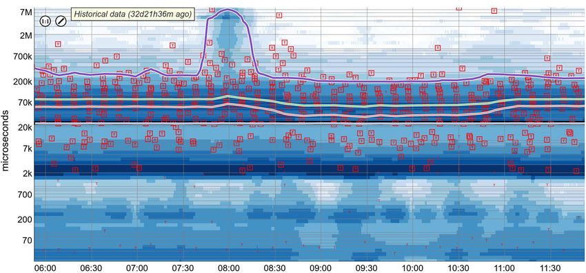
20ms. The 4th point has a new start timestamp; between Figure 4: A heat map of /rpc/server/latency. Click-
10:43 and 10:44, 10 RPCs were served and each took 0–10ms. ing an exemplar shows the captured RPC trace.
3.2 Metrics by its timestamp. For example, /rpc/server/latency in
A metric measures one aspect of a monitored target, such Figure 3 is a cumulative metric: each point is a latency dis-
as the number of RPCs a task has served, the memory uti- tribution of all RPCs from its start time, i.e., the start time
lization of a VM, etc. Similar to a target, a metric conforms of the RPC server. Cumulative metrics are robust in that
to a metric schema, which defines the time series value type they still make sense if some points are missing, because
and a set of metric fields. Metrics are named like files. Fig- each point contains all changes of earlier points sharing the
ure 2 shows an example metric called /rpc/server/latency same start time. Cumulative metrics are important to sup-
that measures the latency of RPCs to a server; it has two port distributed systems which consist of many servers that
metric fields that distinguish RPCs by service and command. may be regularly restarted due to job scheduling [46], where
The value type can be boolean, int64, double, string, points may go missing during restarts.
distribution, or tuple of other types. All of them are
standard types except distribution, which is a compact 4. SCALABLE COLLECTION
type that represents a large number of double values. A To ingest a massive volume of time series data in real
distribution includes a histogram that partitions a set of time, Monarch uses two divide-and-conquer strategies and
double values into subsets called buckets and summarizes one key optimization that aggregates data during collection.
values in each bucket using overall statistics such as mean,
count, and standard deviation [28]. Bucket boundaries are 4.1 Data Collection Overview
configurable for trade-off between data granularity (i.e., ac- The right side of Figure 1 gives an overview of Monarch’s
curacy) and storage costs: users may specify finer buckets collection path. The two levels of routers perform two lev-
for more popular value ranges. Figure 3 shows an exam- els of divide-and-conquer: ingestion routers regionalize time
ple distribution-typed time series of /rpc/server/latency series data into zones according to location fields, and leaf
which measures servers’ latency in handling RPCs; and it routers distribute data across leaves according to the range
has a fixed bucket size of 10ms. Distribution-typed points assigner. Recall that each time series is associated with a
of a time series can have different bucket boundaries; inter- target and one of the target fields is a location field.
polation is used in queries that span points with different Writing time series data into Monarch follows four steps:
bucket boundaries. Distributions are an effective feature for
summarizing a large number of samples. Mean latency is not 1. A client sends data to one of the nearby ingestion
enough for system monitoring—we also need other statistics routers, which are distributed across all our clusters.
such as 99th and 99.9th percentiles. To get these efficiently, Clients usually use our instrumentation library, which
histogram support—aka distribution—is indispensable. automatically writes data at the frequency necessary
Exemplars. Each bucket in a distribution may contain to fulfill retention policies (see Section 6.2.2).
an exemplar of values in that bucket. An exemplar for RPC
metrics, such as /rpc/server/latency, may be a Dapper 2. The ingestion router finds the destination zone based
RPC trace [41], which is very useful in debugging high RPC on the value of the target’s location field, and forwards
latency. Additionally, an exemplar contains information of the data to a leaf router in the destination zone. The
its originating target and metric field values. The informa- location-to-zone mapping is specified in configuration
tion is kept during distribution aggregation, therefore a user to ingestion routers and can be updated dynamically.
can easily identify problematic tasks via outlier exemplars.
Figure 4 shows a heat map of a distribution-typed time se- 3. The leaf router forwards the data to the leaves re-
ries including the exemplar of a slow RPC that may explain sponsible for the target ranges containing the target.
the tail latency spike in the middle of the graph. Within each zone, time series are sharded lexicographi-
Metric types. A metric may be a gauge or a cumu- cally by their target strings (see Section 4.2). Each leaf
lative. For each point of a gauge time series, its value is router maintains a continuously-updated range map
an instantaneous measurement, e.g., queue length, at the that maps each target range to three leaf replicas.
time indicated by the point timestamp. For each point of Note that leaf routers get updates to the range map
a cumulative time series, its value is the accumulation of from leaves instead of the range assigner. Also, target
the measured aspect from a start time to the time indicated ranges jointly cover the entire string universe; all new
3184targets will be picked up automatically without inter- Range assigners balance load in ways similar to Slicer [1].
vention from the assigner. So data collection continues Within each zone, the range assigner splits, merges, and
to work if the assigner suffers a transient failure. moves ranges between leaves to cope with changes in the
CPU load and memory usage imposed by the range on the
4. Each leaf writes data into its in-memory store and re- leaf that stores it. While range assignment is changing, data
covery logs. The in-memory time series store is highly collection works seamlessly by taking advantage of recovery
optimized: it (1) encodes timestamps efficiently and logs. For example (range splits and merges are similar), the
shares timestamp sequences among time series from following events occur once the range assigner decided to
the same target; (2) handles delta and run-length en- move a range, say R, to reduce the load on the source leaf:
coding of time series values of complex types including
distribution and tuple; (3) supports fast read, write, 1. The range assigner selects a destination leaf with light
and snapshot; (4) operates continuously while process- load and assigns R to it. The destination leaf starts to
ing queries and moving target ranges; and (5) mini- collect data for R by informing leaf routers of its new
mizes memory fragmentation and allocation churn. To assignment of R, storing time series with keys within
achieve a balance between CPU and memory [22], the R, and writing recovery logs.
in-memory store performs only light compression such 2. After waiting for one second for data logged by the
as timestamp sharing and delta encoding. Timestamp source leaf to reach disks2 , the destination leaf starts
sharing is quite effective: one timestamp sequence is to recover older data within R, in reverse chronologi-
shared by around ten time series on average. cal order (since newer data is more critical), from the
recovery logs.
Note that leaves do not wait for acknowledgement when
writing to the recovery logs per range. Leaves write logs to 3. Once the destination leaf fully recovers data in R,
distributed file system instances (i.e., Colossus [18]) in mul- it notifies the range assigner to unassign R from the
tiple distinct clusters and independently fail over by prob- source leaf. The source leaf then stops collecting data
ing the health of a log. However, the system needs to con- for R and drops the data from its in-memory store.
tinue functioning even when all Colossus instances are un- During this process, both the source and destination leaves
available, hence the best-effort nature of the write to the are collecting, storing, and logging the same data simulta-
log. Recovery logs are compacted, rewritten into a format neously to provide continuous data availability for the range
amenable for fast reads (leaves write to logs in a write- R. Note that it is the job of leaves, instead of the range as-
optimized format), and merged into the long-term repository signer, to keep leaf routers updated about range assignments
by continuously-running background processes whose details for two reasons: (1) leaves are the source of truth where data
we omit from this paper. All log files are also asynchronously is stored; and (2) it allows the system to degrade gracefully
replicated across three clusters to increase availability. during a transient range assigner failure.
Data collection by leaves also triggers updates in the zone
and root index servers which are used to constrain query 4.3 Collection Aggregation
fanout (see Section 5.4). For some monitoring scenarios, it is prohibitively expen-
sive to store time series data exactly as written by clients.
4.2 Intra-zone Load Balancing One example is monitoring disk I/O, served by millions of
As a reminder, a table schema consists of a target schema disk servers, where each I/O operation (IOP) is accounted
and a metric schema. The lexicographic sharding of data to one of tens of thousands of users in Google. This gener-
in a zone uses only the key columns corresponding to the ates tens of billions of time series, which is very expensive
target schema. This greatly reduces ingestion fanout: in to store naively. However, one may only care about the ag-
a single write message, a target can send one time series gregate IOPs per user across all disk servers in a cluster.
point each for hundreds of different metrics; and having all Collection aggregation solves this problem by aggregating
the time series for a target together means that the write data during ingestion.
message only needs to go to up to three leaf replicas. This Delta time series. We usually recommend clients use
not only allows a zone to scale horizontally by adding more cumulative time series for metrics such as disk IOPs because
leaf nodes, but also restricts most queries to a small subset of they are resilient to missing points (see Section 3.2). How-
leaf nodes. Additionally, commonly used intra-target joins ever, aggregating cumulative values with very different start
on the query path can be pushed down to the leaf-level, times is meaningless. Therefore, collection aggregation re-
which makes queries cheaper and faster (see Section 5.3). quires originating targets to write deltas between adjacent
In addition, we allow heterogeneous replication policies (1 cumulative points instead of cumulative points directly. For
to 3 replicas) for users to trade off between availability and example, each disk server could write to Monarch every TD
storage cost. Replicas of each target range have the same seconds the per-user IOP counts it served in the past TD sec-
boundaries, but their data size and induced CPU load may onds. The leaf routers accept the writes and forward all the
differ because, for example, one user may retain only the first writes for a user to the same set of leaf replicas. The deltas
replica at a fine time granularity while another user retains can be pre-aggregated in the client and the leaf routers, with
all three replicas at a coarse granularity. Therefore, the final aggregation done at the leaves.
range assigner assigns each target range replica individually. 2
Of course, a leaf is never assigned multiple replicas of a single Recall that, to withstand file system failures, leaves do not
wait for log writes to be acknowledged. The one second
range. Usually, a Monarch zone contains leaves in multiple wait length is almost always sufficient in practice. Also,
failure domains (clusters); the assigner assigns the replicas the range assigner waits for the recovery from logs to finish
for a range to different failure domains. before finalizing the range movement.
3185TrueTime.now.latest
1 { fetch ComputeTask ::/ rpc / server / latency
TW 2 | filter user == " monarch "
TB Admission Window 3 | align delta (1 h )
bucket 4 ; fetch ComputeTask ::/ build / label
bucket bucket | filter user == " monarch " && job =~ " mixer .* "
(finalized) 5
x The two latest
6 } | join
The oldest delta is rejected 7 | group_by [ label ] , aggregate ( latency )
because its end time is out delta delta delta deltas are admitted
of the admission window. into the two latest
TD
buckets. Figure 6: An example query of latency distributions
broken down by build label. The underlined are table
Figure 5: Collection aggregation using buckets and operators. delta and aggregate are functions. “=~” de-
a sliding admission window. notes regular expression matching.
Key column: label (aka /build/label) Value column: latency (aka /rpc/server/latency)
Bucketing. During collection aggregation, leaves put
deltas into consecutive time buckets according to the end “mixer-20190105-1” 10:40 10:41 10:42 ...
“mixer-20190105-2” 10:40 10:41 10:42 ...
time of deltas, as illustrated in Figure 5. The bucket length “mixer-20190110-0” 10:40 10:41 10:42 ...
TB is the period of the output time series, and can be con-
figured by clients. The bucket boundaries are aligned differ- Figure 7: An example output time series table.
ently among output time series for load-smearing purposes.
Deltas within each bucket are aggregated into one point ac-
cording to a user-selected reducer; e.g., the disk I/O example The fetch operation on Line 1 reads the time series table
uses a sum reducer that adds up the number of IOPs for a defined by the named target and metric schema from Fig-
user from all disk servers. ure 2. On Line 4, the fetch reads the table for the same
Admission window. In addition, each leaf also main- target schema and metric /build/label whose time series
tains a sliding admission window and rejects deltas older value is a build label string for the target.
than the window length TW . Therefore, older buckets be- The filter operation has a predicate that is evaluated
come immutable and generate finalized points that can be for each time series and only passes through those for which
efficiently stored with delta and run-length encoding. The the predicate is true. The predicate on Line 2 is a single
admission window also enables Monarch to recover quickly equality field predicate on the user field. Predicates can be
from network congestion; otherwise, leaves may be flooded arbitrarily complex, for example combining field predicates
by delayed traffic and never catch up to recent data, which with logical operators as shown on Line 5.
is more important for critical alerting. In practice, rejected The align operation on Line 3 produces a table in which
writes comprise only a negligible fraction of traffic. Once a all the time series have timestamps at the same regularly
bucket’s end time moves out of the admission window, the spaced interval from the same start time. The delta win-
bucket is finalized: the aggregated point is written to the dow operation estimates the latency distribution between
in-memory store and the recovery logs. the time of each aligned output point and one hour ear-
To handle clock skews, we use TrueTime [13] to times- lier. Having aligned input is important for any operation
tamp deltas, buckets, and the admission window. To com- that combines time series, such as join or group by. The
promise between ingestion traffic volume and time series ac- align can be automatically supplied where needed as it is
curacy, the delta period TD is set to 10 seconds in prac- for /build/label (which lacks an explicit align operation).
tice. The length of the admission window is TW = TD + The join operation on Line 6 does a natural (inner) join
TT .now .latest − TT .now .earliest, where TT is TrueTime. on the key columns of the input tables from the queries
The bucket length, 1s ≤ TB ≤ 60s, is configured by clients. separated by the semicolon in the brackets { }. It produces
It takes time TB + TW to finalize a bucket, so recovery logs a table with key columns from both inputs and a time series
are normally delayed by up to around 70 seconds with a max with dual value points: the latency distribution and the
TB of 60 seconds. During range movement, TB is temporar- build label. The output contains a time series for each pair of
ily adjusted to 1 second, since 70 seconds is too long for load input time series whose common key columns match. Left-,
balancing, as the leaf may be overloaded in the meantime. right-, and full-outer joins are also supported.
The group by operation on Line 7 makes the key columns
for each time series to contain only label, the build label.
5. SCALABLE QUERIES It then combines all the time series with the same key (same
To query time series data, Monarch provides an expres- build label) by aggregating the distribution values, point by
sive language powered by a distributed engine that localizes point. Figure 7 shows its results.
query execution using static invariants and a novel index. The operations in Figure 6 are a subset of the available
operations, which also include the ability to choose the top
5.1 Query Language n time series according to a value expression, aggregate val-
A Monarch query is a pipeline of relational-algebra-like ues across time as well as across different time series, remap
table operations, each of which takes zero or more time se- schemas and modify key and value columns, union input ta-
ries tables as input and produces a single table as output. bles, and compute time series values with arbitrary expres-
Figure 6 shows a query that returns the table shown in Fig- sions such as extracting percentiles from distribution values.
ure 7: the RPC latency distribution of a set of tasks broken
down by build labels (i.e., binary versions). This query can 5.2 Query Execution Overview
be used to detect abnormal releases causing high RPC la- There are two kinds of queries in the system: ad hoc
tency. Each line in Figure 6 is a table operation. queries and standing queries. Ad hoc queries come from
3186users outside of the system. Standing queries are periodic 5.3 Query Pushdown
materialized-view queries whose results are stored back into Monarch pushes down evaluation of a query’s table opera-
Monarch; teams use them: (1) to condense data for faster tions as close to the source data as possible. This pushdown
subsequent querying and/or cost saving; and (2) to generate uses static invariants on the data layout, derived from the
alerts. Standing queries can be evaluated by either regional target schema definition, to determine the level at which an
zone evaluators or global root evaluators. The decision is operation can be fully completed, with each node in this
based on static analysis of the query and the table schemas level providing a disjoint subset of all output time series
of the inputs to the query (details in Section 5.3). The ma- for the operation. This allows the subsequent operations to
jority of standing queries are evaluated by zone evaluators start from that level. Query pushdown increases the scale
which send identical copies of the query to the correspond- of queries that can be evaluated and reduces query latency
ing zone mixers and write the output to their zone. Such because (1) more evaluation at lower levels means more con-
queries are efficient and resilient to network partition. The currency and evenly distributed load; and (2) full or partial
zone and root evaluators are sharded by hashes of stand- aggregations computed at lower levels substantially decrease
ing queries they process, allowing us to scale to millions of the amount of data transferred to higher level nodes.
standing queries. Pushdown to zone. Recall that data is routed to zones
Query tree. As shown in Figure 1, global queries are by the value in the location target field. Data for a specific
evaluated in a tree hierarchy of three levels. A root mixer location can live only in one zone. If an output time series
receives the query and fans out to zone mixers, each of which of an operation only combines input time series from a sin-
fans out to leaves in that zone. The zonal standing queries gle zone, the operation can complete at the zone level. For
are sent directly to zone mixers. To constrain the fanout, example, a group by where the output time series keys con-
root mixers and zone mixers consult the index servers for tain the location field, and a join between two inputs with
a set of potentially relevant children for the query (see Sec- a common location field can both be completed at the zone
tion 5.4). A leaf or zone is relevant if the field hints index level. Therefore, the only standing queries issued by the root
indicates that it could have data relevant to the query. evaluators are those that either (a) operate on some input
Level analysis. When a node receives a query, it de- data in the regionless zone which stores the standing query
termines the levels at which each query operation runs and results with no location field, or (b) aggregate data across
sends down only the parts to be executed by the lower levels zones, for example by either dropping the location field in
(details in Section 5.3). In addition, the root of the execu- the input time series or by doing a top n operation across
tion tree performs security and access-control checks and time series in different zones. In practice, this allows up to
potentially rewrites the query for static optimization. Dur- 95% of standing queries to be fully evaluated at zone level
ing query execution, lower-level nodes produce and stream by zone evaluators, greatly increasing tolerance to network
the output time series to the higher-level nodes which com- partition. Furthermore, this significantly reduces latency by
bine the time series from across their children. Higher-level avoiding cross-region writes from root evaluators to leaves.
nodes allocate buffer space for time series from each par- Pushdown to leaf. As mentioned in Section 4.2, the
ticipating child according to the network latency from that data is sharded according to target ranges across leaves within
child, and control the streaming rate by a token-based flow a zone. Therefore, a leaf has either none or all of the data
control algorithm. from a target. Operations within a target complete at the
Replica resolution. Since the replication of data is leaf level. For example, a group by that retains all the tar-
highly configurable, replicas may retain time series with dif- get fields in the output and a join whose inputs have all the
ferent duration and frequency. Additionally, as the target target fields can both complete at the leaf level. Intra-target
ranges may be moving (see Section 4.2), some replicas can joins are very common in our monitoring workload, such as
be in recovery with incomplete data. To choose the leaf with filtering with slow changing metadata time series stored in
the best quality of data in terms of time bounds, density, and the same target. In the example query in Figure 6, the join
completeness, zonal queries go through the replica resolution completes at the leaf and /build/label can be considered
process before processing data. Relevant leaves return the as metadata (or a property) of the target (i.e., the running
matched targets and their quality summary, and the zone task), which changes only when a new version of the binary
mixer shards the targets into target ranges, selecting for is pushed. In addition, since a target range contains con-
each range a single leaf based on the quality. Each leaf then secutive targets (i.e., the first several target fields might be
evaluates the table operations sent to it for the target range identical for these targets), a leaf usually contains multiple
assigned to it. Though the range assigner has the target targets relevant to the query. Aggregations are pushed down
information, replica resolution is done purely from the tar- as much as possible, even when they cannot be completed
get data actually on each leaf. This avoids a dependency on at the leaf level. The leaves aggregate time series across
the range assigner and avoids overloading it. While process- the co-located targets and send these results to the mixers.
ing queries, relevant data may be deleted because of range The group by in the example query is executed at all three
movements and retention expiration; to prevent that, leaves levels. No matter how many input time series there are for
take a snapshot of the input data until queries finish. each node, the node only outputs one time series for each
User isolation. Monarch runs as a shared service; the group (i.e., one time series per build label in the example).
resources on the query execution nodes are shared among Fixed Fields. Some fields can be determined to fix to
queries from different users. For user isolation, memory used constant values by static analysis on the query and schemas,
by queries is tracked locally and across nodes, and queries and they are used to push down more query operations. For
are cancelled if a user’s queries use too much memory. Query example, when fetching time series from a specific cluster
threads are put into per-user cgroups [45], each of which is with a filter operation of filter cluster == "om", a global
assigned a fair share of CPU time. aggregation can complete at the zone level, because the in-
3187put time series are stored in only one zone that contains the string fields with small character sets (e.g. ISBN) can
specific cluster value om. be configured to use fourgrams and full strings, in ad-
dition to trigrams, as excerpts for higher accuracy.
5.4 Field Hints Index
For high scalability, Monarch uses field hints index (FHI), 3. Monarch combines static analysis and FHIs to further
stored in index servers, to limit the fanout when sending a reduce the fanout of queries with joins: it sends the
query from parent to children, by skipping irrelevant chil- example query (which contains a leaf-level inner join)
dren (those without input data to the particular query). only to leaves satisfying both of the two filter predicates
An FHI is a concise, continuously-updated index of time in Figure 6 (the join will only produce output on such
series field values from all children. FHIs skip irrelevant leaves anyway). This technique is similarly applied to
children by analyzing field predicates from queries, and han- queries with nested joins of varying semantics.
dle regular expression predicates efficiently without iterating
4. Metric names are also indexed, by full string, and are
through the exact field values. FHI works with zones with
treated as values of a reserved “:metric” field. Thus,
trillions of time series keys and more than 10,000 leaves while
FHIs even help queries without any field predicates.
keeping the size small enough to fit in memory. False posi-
tives are possible in FHI just as in Bloom filters [7]; that is,
As illustrated in Figure 1, FHIs are built from bottom up
FHIs may also return irrelevant children. False positives do
and maintained in index servers. Due to its small size, an
not affect correctness because irrelevant children are ignored
FHI need not be stored persistently. It is built (within min-
via replica resolution later.
utes) from live leaves when an index server starts. A zone
A field hint is an excerpt of a field value. The most com-
index server maintains a long-lived streaming RPC [26] to
mon hints are trigrams; for example, ^^m, ^mo, mon, ona,
every leaf in the zone for continuous updates to the zone
nar, arc, rch, ch$, and h$$ are trigram hints of field value
FHI. A root index server similarly streams updates to the
monarch where ^ and $ represent the start and end of text,
root FHI from every zone. Field hints updates are trans-
respectively. A field hint index is essentially a multimap that
ported over the network at high priority. Missing updates
maps the fingerprint of a field hint to the subset of children
to the root FHI are thus reliable indicators of zone unavail-
containing the hint. A fingerprint is an int64 generated
ability, and are used to make global queries resilient to zone
deterministically from three inputs of a hint: the schema
unavailability.
name, the field name, and the excerpt (i.e., trigrams).
Similar Index Within Each Leaf. Field hints index in-
When pushing down a query, a root (zone) mixer extracts
troduced so far resides in index servers and helps each query
a set of mandatory field hints from the query, and looks
to locate relevant leaves. Within each leaf, there is a similar
up the root (zone) FHI for the destination zones (leaves).
index that helps each query to find relevant targets among
Take the query in Figure 6 for example: its predicate reg-
the large number of targets the leaf is responsible for. To
exp ‘mixer.*’ entails ^^m, ^mi, mix, ixe, and xer. Any
summarize, a query starts from the root, uses root-level FHI
child matching the predicate must contain all these trigrams.
in root index servers to find relevant zones, then uses zone-
Therefore, only children in FHI[^^m] ∩ FHI[^mi] ∩ FHI[mix]
level FHI in zone index servers to find relevant leaves, and
∩ FHI[ixe] ∩ FHI[xer] need to be queried.
finally uses leaf-level FHI in leaves to find relevant targets.
We minimize the size of FHI to fit it in memory so that
Monarch still works during outages of secondary storage sys- 5.5 Reliable Queries
tems. Storing FHI in memory also allows fast updates and
As a monitoring system, it is especially important for
lookups. FHI trades accuracy for a small index size: (1)
Monarch to handle failures gracefully. We already discussed
It indexes short excerpts to reduce the number of unique
that Monarch zones continue to function even during fail-
hints. For instance, there are at most 263 unique trigrams
ures of the file system or global components. Here we discuss
for lowercase letters. Consequently, in the previous example,
how we make queries resilient to zonal and leaf-level failures.
FHI considers a leaf with target job:‘mixixer’ relevant al-
Zone pruning. At the global level, we need to protect
though the leaf’s target does not match regexp ‘mixer.*’.
global queries from regional failures. Long-term statistics
(2) FHI treats each field separately. This causes false posi-
show that almost all (99.998%) successful global queries
tives for queries with predicates on multiple fields. For ex-
start to stream results from zones within the first half of
ample, a leaf with two targets user:‘monarch’,job:‘leaf’
their deadlines. This enabled us to enforce a shorter per-
and user:‘foo’,job:‘mixer.root’ is considered by FHI
zone soft query deadline as a simple way of detecting the
a match for predicate user==‘monarch’&&job=~‘mixer.*’
health of queried zones. A zone is pruned if it is completely
(Figure 6) although neither of the two targets actually match.
unresponsive by the soft query deadline. This gives each
Despite their small sizes (a few GB or smaller), FHIs re-
zone a chance to return responses but not significantly de-
duce query fanout by around 99.5% at zone level and by
lay query processing if it suffers from low availability. Users
80% at root level. FHI also has four additional features:
are notified of pruned zones as part of the query results.
1. Indexing trigrams allows FHIs to filter queries with Hedged reads. Within a zone, a single query may still
regexp-based field predicates. The RE2 library can fanout to more than 10,000 leaves. To make queries resilient
turn a regexp into a set algebra expression with tri- to slow leaf nodes, Monarch reads data from faster replicas.
grams and operations (union and intersection) [14]. To As described in Section 4.2, leaves can contain overlapping
match a regexp predicate, Monarch simply looks up its but non-identical sets of targets relevant to a query. As
trigrams in FHIs and evaluates the expression. we push down operations that can aggregate across all the
relevant targets at the leaf (see Section 5.3), there is no
2. FHIs allow fine-grained tradeoff between index accu- trivial output data equivalence across leaves. Even when
racy and size by using different excerpts. For instance, leaves return the same output time series keys, they might be
3188aggregations from different input data. Therefore, a vanilla Table 1: Number of Monarch tasks by component,
hedged read approach does not work. rounded to the third significant digit. Components for
Monarch constructs the equivalence of input data on the logging, recovery, long-term repository, quota management,
query path with a novel hedged-read approach. As men- and other supporting services are omitted.
tioned before, the zone mixer selects a leaf (called the pri- Component #Task Component #Task
mary leaf ) to run the query for each target range during Leaf 144,000 Range assigner 114
replica resolution. The zone mixer also constructs a set of Config mirror 2,590 Config server 15
fallback leaves for the responsible ranges of each primary Leaf router 19,700 Ingestion router 9,390
leaf. The zone mixer starts processing time series reads from Zone mixer 40,300 Root mixer 1,620
Zone index server 3,390 Root index server 139
the primary leaves while tracking their response latencies. If Zone evaluator 1,120 Root evaluator 36
a primary leaf is unresponsive or abnormally slow, the zone
mixer replicates the query to the equivalent set of fallback
leaves. The query continues in parallel between the primary in Section 3, that allow data to be collected automatically
leaf and the fallback leaves, and the zone mixer extracts and for common workloads and libraries. Advanced users can
de-duplicates the responses from the faster of the two. define their own custom target schemas, providing the flex-
ibility to monitor many types of entities.
6. CONFIGURATION MANAGEMENT Monarch provides a convenient instrumentation library
Due to the nature of running Monarch as a distributed, for users to define schematized metrics in code. The library
multi-tenant service, a centralized configuration manage- also periodically sends measurements as time series points
ment system is needed to give users convenient, fine-grained to Monarch as configured in Section 6.2.2. Users can con-
control over their monitoring and distribute configuration veniently add columns as their monitoring evolves, and the
throughout the system. Users interact with a single global metric schema will be updated automatically. Users can set
view of configuration that affects all Monarch zones. access controls on their metric namespace to prevent other
users from modifying their schemas.
6.1 Configuration Distribution
All configuration modifications are handled by the con- 6.2.2 Collection, Aggregation, and Retention
figuration server, as shown in Figure 1, which stores them Users have fine-grained control over data retention poli-
in a global Spanner database [13]. A configuration element cies, i.e., which metrics to collect from which targets and
is validated against its dependencies (e.g., for a standing how to retain them. They can control how frequently data is
query, the schemas it uses) before being committed. sampled, how long it is retained, what the storage medium
The configuration server is also responsible for transform- is, and how many replicas to store. They can also down-
ing high-level configuration to a form that is more efficiently sample data after a certain age to reduce storage costs.
distributed and cached by other components. For example, To save costs further, users can also configure aggregation
leaves only need to be aware of the output schema of a stand- of metrics during collection as discussed in Section 4.3.
ing query to store its results. Doing this transformation
within the configuration system itself ensures consistency 6.2.3 Standing Queries
across Monarch components and simplifies client code, re- Users can set up standing queries that are evaluated pe-
ducing the risk of a faulty configuration change taking down riodically and whose results are stored back into Monarch
other components. Dependencies are tracked to keep these (Section 5.2). Users can configure their standing query to
transformations up to date. execute in a sharded fashion to handle very large inputs.
Configuration state is replicated to configuration mirrors Users can also configure alerts, which are standing queries
within each zone, which are then distributed to other com- with a boolean output comparing against user-defined alert-
ponents within the zone, making it highly available even in ing conditions. They also specify how to be notified (e.g.,
the face of network partitions. Zonal components such as email or page) when alerting conditions are met.
leaves cache relevant configuration in memory to minimize
latency of configuration lookups, which are copied from the
configuration mirror at startup with subsequent changes be- 7. EVALUATION
ing sent periodically. Normally the cached configuration is Monarch has many experimental deployments and three
up to date, but if the configuration mirror becomes unavail- production deployments: internal, external, and meta. In-
able, zonal components can continue to operate, albeit with ternal and external are for customers inside and outside
stale configuration and our SREs alerted. Google; meta runs a proven-stable older version of Monarch
and monitors all other Monarch deployments. Below, we
6.2 Aspects of Configuration only present numbers from the internal deployment, which
Predefined configuration is already installed to collect, does not contain external customer data. Note that Mon-
query, and alert on data for common target and metric arch’s scale is not merely a function of the scale of the sys-
schemas, providing basic monitoring to new users with min- tems being monitored. In fact, it is significantly more influ-
imal setup. Users can also install their own configuration to enced by other factors such as continuous internal optimiza-
utilize the full flexibility of Monarch. The following subsec- tions, what aspects are being monitored, how much data is
tions describe major parts of users’ configuration state: aggregated, etc.
6.2.1 Schemas 7.1 System Scale
There are predefined target schemas and metric schemas, Monarch’s internal deployment is in active use by more
such as ComputeTask and /rpc/server/latency as described than 30,000 employees and teams inside Google. It runs in
31891000 800 8
Count (Billion)
QPS (Million)
800
Size (TB)
600 6
600
400 4
400
200 200 2
0 0 0
6-07 7-01 7-07 8-01 8-07 9-01 9-07 6-07 7-01 7-07 8-01 8-07 9-01 9-07 6-07017-01017-07018-01018-07019-01019-07
201 201 201 201 201 201 201 201 201 201 201 201 201 201 201 2 2 2 2 2 2
Figure 8: Time series count. Figure 9: Time series memory size. Figure 10: Queries per second.
Write Rate (TB/s)
2.5 Table 2: Field hints index (FHI) statistics. Children
2 of the root FHI are the 38 zones. Zone FHIs are named after
1.5 the zone, and their children are leaves. Suppression ratio is
1 the percentage of children skipped by query thanks to FHI.
0.5 Hit ratio is the percentage of visited children that actually
0
have data. 26 other zones are omitted.
6-07 7-01 7-07 8-01 8-07 9-01 9-07
201 201 201 201 201 201 201
FHI Name Child Fingerprint Suppr. Hit
Figure 11: Time series data written per second. The Count Count (k) Ratio Ratio
write rate was almost zero around July 2016 because back root 38 214,468 75.8 45.0
then data was ingested using a different mechanism, which small-zone-1 15 56 99.9 60.5
is not included in this figure. Detailed measurement of the small-zone-2 56 1,916 99.7 51.8
small-zone-3 96 3,849 99.5 43.8
old mechanism is no longer available; its traffic peaked at
medium-zone-1 156 6,377 99.4 36.3
around 0.4TB/s, gradually diminished, and became negligi- medium-zone-2 330 12,186 99.5 32.9
ble around March 2018. medium-zone-3 691 23,404 99.2 33.4
large-zone-1 1,517 43,584 99.3 26.5
large-zone-2 5,702 159,090 99.2 22.5
large-zone-3 7,420 280,816 99.3 21.6
38 zones spread across five continents. It has round 400,000 huge-zone-1 12,764 544,815 99.4 17.8
tasks (the important ones are listed in Table 1), with the huge-zone-2 15,475 654,750 99.4 18.4
vast majority of tasks being leaves because they serve as the huge-zone-3 16,681 627,571 99.6 21.4
in-memory time series data store. Classifying zones by the
number of leaves, there are: 5 small zones (< 100 leaves),
16 medium zones (< 1000), 11 large zones (< 10, 000), and 7.2 Scalable Queries
6 huge zones (≥ 10, 000). Each zone contains three range
assigners, one of which is elected to be the master. Other To evaluate query performance, we present key statistics
components in Table 1 (config, router, mixer, index server, about query pushdown, field hints index (FHI, Section 5.4),
and evaluator) appear at both zone and root levels; the and query latency. We also examine the performance impact
root tasks are fewer than the zone counterparts because root of various optimizations using an example query.
tasks distribute work to zone tasks as much as possible.
Monarch’s unique architecture and optimizations make it 7.2.1 Overall Query Performance
highly scalable. It has sustained fast growth since its in- Figure 10 shows the query rate of Monarch’s internal de-
ception and is still growing rapidly. Figure 8 and Figure 9 ployment: it has sustained exponential growth and was serv-
show the number of time series and the bytes they consume ing over six million QPS as of July 2019. Approximately
in Monarch’s internal deployment. As of July 2019, Mon- 95% of all queries are standing queries (including alerting
arch stored nearly 950 billion time series, consuming around queries). This is because users usually set up standing
750TB memory with a highly-optimized data structure. Ac- queries (1) to reduce response latency for queries that are
commodating such growth rates requires not only high hori- known to be exercised frequently and (2) for alerting, whereas
zontal scalability in key components but also innovative op- they only issue ad hoc non-standing-queries very occasion-
timizations for collection and query, such as collection ag- ally. Additionally, the majority of such standing queries are
gregation (Section 4.3) and field hints index (Section 5.4). initiated by the zone evaluators (as opposed to the root eval-
As shown in Figure 11, Monarch’s internal deployment uators) because Monarch aggressively pushes down those
ingested around 2.2 terabytes of data per second in July standing queries that can be independently evaluated in each
2019. Between July 2018 and January 2019, the ingestion zone to the zone evaluators to reduce the overall amount of
rate almost doubled because collection aggregation enabled unnecessary work performed by the root evaluators.
collection of metrics (e.g., disk I/O) with tens of billions of To quantify the query pushdown from zone mixers to
time series keys. On average, Monarch aggregates 36 input leaves, we measured that the overall ratio of output to in-
time series into one time series during collection; in extreme put time series count at leaves is 23.3%. Put another way,
cases, over one million input time series into one. Collection pushdown reduces the volume of data seen by zone mixers
aggregation is highly efficient and can aggregate one million by a factor of four.
typical time series using only a single CPU core. In addition Besides query pushdown, field hints index is another key
to the obvious RAM savings (fewer time series to store), enabler for scalable queries. Table 2 shows the statistics of
collection aggregation uses approximately 25% of the CPU the root and some zone FHIs. The root FHI contains around
of the alternative procedure of writing the raw time series to 170 million fingerprints; it narrows average root query fanout
Monarch, querying via a standing query, and then writing down to 34×(1−0.758) ≈ 9, among which around 9×0.45 ≈
the desired output. 4 zones actually have data. Zones vary a lot in their leaf
3190You can also read