Ten-year return levels of sub-daily extreme precipitation over Europe - ESSD
←
→
Page content transcription
If your browser does not render page correctly, please read the page content below
Earth Syst. Sci. Data, 13, 983–1003, 2021
https://doi.org/10.5194/essd-13-983-2021
© Author(s) 2021. This work is distributed under
the Creative Commons Attribution 4.0 License.

                              Ten-year return levels of sub-daily
                              extreme precipitation over Europe
                                  Benjamin Poschlod1 , Ralf Ludwig1 , and Jana Sillmann2
             1 Department    of Geography, Ludwig-Maximilians-Universität München, 80333 Munich, Germany
              2 Center   for International Climate and Environmental Research (CICERO), Oslo, 0318, Norway
                            Correspondence: Benjamin Poschlod (Benjamin.Poschlod@lmu.de)

                                      Received: 8 June 2020 – Discussion started: 4 August 2020
                          Revised: 26 January 2021 – Accepted: 8 February 2021 – Published: 11 March 2021

      Abstract. Information on the frequency and intensity of extreme precipitation is required by public authorities,
      civil security departments, and engineers for the design of buildings and the dimensioning of water management
      and drainage schemes. Especially for sub-daily resolutions, at which many extreme precipitation events occur,
      the observational data are sparse in space and time, distributed heterogeneously over Europe, and often not pub-
      licly available. We therefore consider it necessary to provide an impact-orientated data set of 10-year rainfall
      return levels over Europe based on climate model simulations and evaluate its quality. Hence, to standardize
      procedures and provide comparable results, we apply a high-resolution single-model large ensemble (SMILE)
      of the Canadian Regional Climate Model version 5 (CRCM5) with 50 members in order to assess the frequency
      of heavy-precipitation events over Europe between 1980 and 2009. The application of a SMILE enables a ro-
      bust estimation of extreme-rainfall return levels with the 50 members of 30-year climate simulations providing
      1500 years of rainfall data. As the 50 members only differ due to the internal variability in the climate system,
      the impact of internal variability on the return level values can be quantified.
         We present 10-year rainfall return levels of hourly to 24 h durations with a spatial resolution of 0.11◦ (12.5 km),
      which are compared to a large data set of observation-based rainfall return levels of 16 European countries. This
      observation-based data set was newly compiled and homogenized for this study from 32 different sources. The
      rainfall return levels of the CRCM5 are able to reproduce the general spatial pattern of extreme precipitation
      for all sub-daily durations with Spearman’s rank correlation coefficients > 0.76 for the area covered by obser-
      vations. Also, the rainfall intensity of the observational data set is in the range of the climate-model-generated
      intensities in 60 % (77 %, 78 %, 83 %, 78 %) of the area for hourly (3, 6, 12, 24 h) durations. This results in biases
      between −16.3 % (hourly) to +8.2 % (24 h) averaged over the study area. The range, which is introduced by the
      application of 50 members, shows a spread of −15 % to +18 % around the median.
         We conclude that our data set shows good agreement with the observations for 3 to 24 h durations in large
      parts of the study area. However, for an hourly duration and topographically complex regions such as the Alps
      and Norway, we argue that higher-resolution climate model simulations are needed to improve the results. The
      10-year return level data are publicly available (Poschlod, 2020; https://doi.org/10.5281/zenodo.3878887).

Published by Copernicus Publications.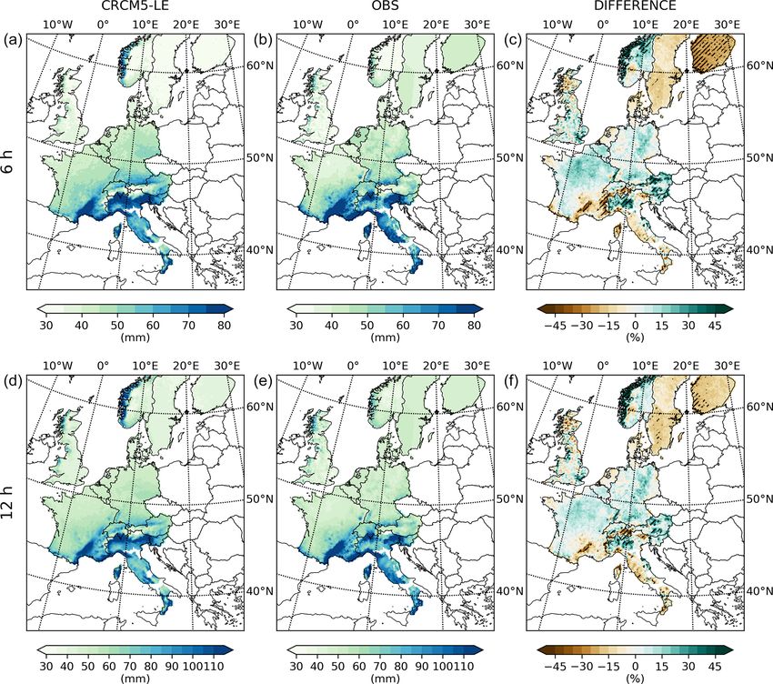
984                                  B. Poschlod et al.: Ten-year return levels of sub-daily extreme precipitation over Europe

1   Introduction                                                    by the Global Sub-Daily Rainfall Dataset (GSDR; Lewis et
                                                                    al., 2019a), which was not yet accessible during the conduct
Sub-daily precipitation extremes affect our daily lives with        of this study. However, the GSDR provides in situ data cov-
a wide range of consequences that can have impacts on in-           ering limited time periods and participating countries only.
frastructure, economy, and even health. Short-duration events          Therefore, we see a need to generate a homogeneous data
of minutes and up to several hours can cause urban flood-           set of rainfall return levels over Europe based on climate
ing, trigger landslides, flash floods, and snow avalanches or       model simulations and to evaluate its quality. We choose
induce heavy erosion (Arnbjerg-Nielsen et al., 2013; Bruni          10-year return periods of hourly and 3, 6, 12, and 24 h du-
et al., 2015; Gill and Malamud, 2014; Marchi et al., 2010;          rations. The limited time period of observational data sug-
Ochoa-Rodriguez et al., 2015; Panagos et al., 2017). Heavy-         gests that a relatively moderate return period should be cho-
rainfall events of several hours and up to days can lead to         sen to ensure comparability with observations. Additionally,
river flooding or coastal flooding as a singular trigger or as      the 10-year return level as a threshold for the detection of
a contributing process of compound flooding events such as          extreme events has already been chosen by Nissen and Ul-
rain-on-snow or coastal compound floods due to joint river          brich (2017) based on legislation and stakeholder interviews.
runoff and storm surge (Bevacqua et al., 2017, 2019; Co-            Also, the recent study of Berg et al. (2019) calculates this
hen et al., 2015; van den Hurk et al., 2015; Poschlod et al.,       return level for nine selected regional climate models of the
2020). These hazards have large impacts on the European in-         EURO-CORDEX multimodel ensemble.
frastructure of urban drainage systems, roads and railroads,           The durations between 1 h and 24 h cover a variety of
waterway transport, electricity, and communication networks         rainfall-generating mechanisms such as convection, advec-
(Forzieri et al., 2018; Groenemeijer et al., 2015; Nissen and       tion, and orographic precipitation. The complexity of these
Ulbrich, 2017). The agricultural sector is directly affected        processes inducing extreme precipitation, their inherent in-
by flooded crop fields and therefore lost yields and in the         termittency properties, and their variability are still not well
longer term by eroding soils and leaching nutrients (Mäki-          understood and a matter for recent climate and weather re-
nen et al., 2018; Panagos et al., 2017). Due to increased           search (Trenberth et al., 2017; Das et al., 2020). Hence, the
settlement in flood-prone areas, the financial impact on the        comparison to observational data is also relevant for the eval-
economic, societal, and private sector has risen in Europe          uation of the process knowledge within the regional climate
over the past decades (Barredo, 2009; Forzieri et al., 2018;        model and the applied parametrization schemes.
Rojas et al., 2013). Human health is also affected, as these
hazards can cause accidents or even fatalities (Krøgli et al.,
                                                                    2     Data and methods
2018; Petrucci et al., 2019). The Munich Re NatCatSER-
VICE reports financial losses of around EUR 173 billion for         2.1    The Canadian Regional Climate Model version 5
the 33 member states of the European Environment Agency                    Large Ensemble (CRCM5-LE)
between 1980 and 2017 due to floods and mass movements
(EEA, 2019). Over 4600 people have lost their lives because         The global climate for this study is based on a large ensem-
of these hazards.                                                   ble of global climate model (GCM) simulations, which was
   Hence, we conclude that the frequency and intensity of           performed with the Canadian Earth System Model version
heavy-precipitation events as triggers of high-impact floods,       2 (CanESM2) at the rather broad spatial resolution of 2.8◦
mass movements, and erosion is of great financial and soci-         (Arora et al., 2011; Fyfe et al., 2017). The CanESM2 was run
etal relevance. In this study, we analyse precipitation dynam-      for 1000 years forced by constant preindustrial conditions.
ics at the sub-daily timescale. For these durations, the obser-     After applying small random atmospheric perturbations, five
vational network for precipitation over Europe is distributed       runs with differing initial conditions were set up starting in
quite heterogeneously. The density of observations is sparse,       January 1850 (Leduc et al., 2019). On 1 January 1950, 10
and the time periods of observed data are often too short to        new random atmospheric perturbations were applied to each
assess extreme events (Lewis et al., 2019a). The data avail-        of the five runs resulting in an ensemble of 50 members
ability is limited and the “data processing stage” varies for       in sum. These 50 simulations were forced with estimations
each country or even region. The provided rainfall products         of historical CO2 and non-CO2 greenhouse gas emissions,
cover the range of in situ annual maxima of sub-daily precip-       aerosol concentrations, and land use until December 2005
itation, in situ time series of sub-daily precipitation, in situ    (Arora et al., 2011). From 2006 to 2099, the climate pro-
return levels, areal time series, and areal return levels. It de-   jections follow the radiative forcing from the representative
pends on the respective meteorological office if the data are       concentration pathway (RCP) 8.5.
available via open access or only by registration and in which         Implementing slight atmospheric perturbations in 1850
format the data are provided. Additionally, access to the data      and 1950 results in different climate realizations, though
is often complicated by the fact that the relevant information,     neither the atmospheric forcing nor the model dynamics,
often provided on websites or data sheets, is only available in     physics, or structure was changed (Arora et al., 2011). The
the national language. These difficulties may be partly solved      climate projections only differ due to the internal variability

Earth Syst. Sci. Data, 13, 983–1003, 2021                                            https://doi.org/10.5194/essd-13-983-2021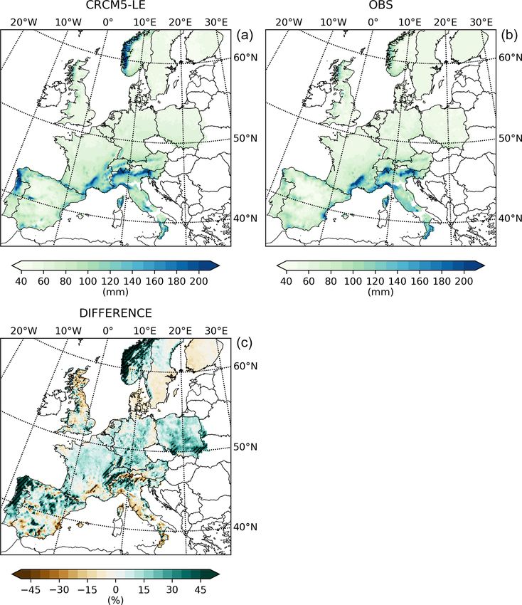
B. Poschlod et al.: Ten-year return levels of sub-daily extreme precipitation over Europe                                    985

in the climate system, which is caused by non-linear dynam-       the west coasts of Spain, Portugal, Ireland, the UK, Norway,
ical processes intrinsic to the atmosphere (Deser et al., 2012;   Croatia, Albania, and Greece and in the topographically com-
Hawkins and Sutton, 2009; von Trentini et al., 2019).             plex areas of the Alps, Carpathians, and Pyrenees (Leduc et
   The framework for the design of the single-model large         al., 2019). These precipitation biases are in the range of the
ensemble (SMILE) of the regional climate model (RCM) as           EURO-CORDEX models as well (Kotlarski et al., 2014).
well as the simulations of the CRCM5-LE were then car-
ried out within the ClimEx project (Climate Change and Hy-        2.2   Calculation of rainfall return periods
drological Extreme Events – Risks and Perspectives for Wa-
ter Management in Bavaria and Québec). Each of the 50             In climate science, extreme precipitation is mostly assessed
CanESM2 simulations were dynamically downscaled with              via the analysis of high quantiles, such as the 99.7 % quan-
the CRCM5 applying the EURO-CORDEX grid specifica-                tile, which equals the occurrence probability of an event hap-
tions (0.11◦ horizontal resolution equalling around 12.5 km).     pening once per year (Santos et al., 2016; Hennemuth et al.,
   The precipitation-related physical parametrization             2013). Risk analysis, engineering guidelines, and also leg-
schemes in the CRCM5 setup include the following mod-             islative thresholds are often expressed as return levels. Ap-
ules (Bresson et al., 2017; Martynov et al., 2012, 2013):         plying extreme value theory (EVT), return periods can be
subgrid-scale orographic gravity-wave drag by McFarlane           calculated by fitting extreme value distributions to a selec-
(1987) is implemented, and low-level orographic blocking is       tion of independent and identically distributed samples of ex-
parametrized via Zadra et al. (2003). The planetary boundary      treme events (Coles, 2001). EVT consists of the two funda-
layer scheme (Benoit et al., 1989; Delage, 1997; Delage and       mentally different sampling strategies block maxima (BM)
Girard, 1992) was used in a modified version by McTaggart-        and peak over threshold (POT). By choosing annual block
Cowan and Zadra (2015) in order to introduce hysteresis           maxima as a sampling strategy, we ensure that the extreme
effects. The Sundquist (Sundquist, 1978; Sundquist et             samples are independent from each other. Still, sampling
al., 1989) scheme is applied as a condensation scheme             only one event per year may result in a loss of information
to diagnose large-scale precipitation. Shallow convection         compared to the POT approach. Also, lower-intensity obser-
is parametrized with the Kuo transient scheme (Bélair et          vations, which are not extreme but still the maximum value
al., 2005; Kuo, 1965), and deep convection is described           of the year, may be included due to the application of the BM
with the Kain and Fritsch (1990) scheme. Land surface             strategy.
processes are simulated by the Canadian Land Surface                 Due to the hourly resolution of the CRCM5-LE data, the
Scheme, version 3.5 (CLASS3.5; Verseghy, 1991, 2009),             hourly maxima are constrained to the fixed window at the full
and lakes are modelled with the one-dimensional freshwater        hour (e.g. 06:00 to 07:00). For all other durations (3, 6, 12,
lake model (FLake; Martynov et al., 2012, 2013). For the          and 24 h, respectively) we allow hourly moving windows for
details of the whole CRCM5 setup the reader may refer to          the selection of maxima.
Martynov et al. (2012) or Hernández-Díaz et al. (2012).              We applied a Mann–Kendall test with p = 0.05 (0.01) on
   RCM SMILEs are relatively rare due to the high demands         the 50 series of 30 annual maxima and five different durations
on computing power. In addition to the CRCM5-LE only the          revealing a trend for less than 6 % (1 %) of all grid cells over
21-member CESM-COSMO-CLM SMILE with a horizon-                    all durations. The affected grid cells vary in location within
tal spatial resolution of 0.44◦ (Addor and Fischer, 2015) and     the 50 climate model simulations, and we therefore do not
the 16-member EC-EARTH-RACMO2 SMILE with a hor-                   apply any de-trending methods.
izontal spatial resolution of 0.11◦ (Aalbers et al., 2018) are       Following the Fisher–Tippett theorem, the distribution of
available for a European domain. Although newer model ver-        block maxima samples converges to the generalized extreme
sions are already available, such as CanESM5 (Swart et al.,       value (GEV) distribution Eq. (1):
2019), the existing CRCM5-LE provides a unique database                       (                   −1/ξ
with the highest number of members, largest domain, and                         exp − 1 + ξ x−µ  σ           ,    ξ 6= 0
                                                                  G(x; ξ ) =                   x−µ
                                                                                                                         ,     (1)
highest spatial resolution available.                                           exp − exp − σ         ,           ξ =0
   In this study, we focus on the precipitation during the time
period of 1980 to 2009, which is simulated by the CRCM5           where µ, σ , and ξ represent the location, scale, and shape
and stored in an hourly resolution. Hence, for the calcula-       parameters of the distribution. The shape parameter ξ gov-
tion of return periods, 1500 years of hourly precipitation un-    erns the tail behaviour of the GEV distribution. According
der conditions of this climate period are available. Leduc et     to the value of ξ , the GEV corresponds to the Gumbel (ξ =
al. (2019) evaluate mean precipitation during 1980 to 2012        0), Fréchet (ξ > 0), or Weibull (ξ < 0) distribution (Coles,
by comparing the annual rainfall with E-OBS data over the         2001). We fit the location, scale, and shape parameters sep-
whole European domain. Generally, the CRCM5-LE shows              arately for each of the 50 differing 30-year block maxima
a wet bias in mean precipitation of up to 2 mm d−1 during         via the method of L-moments (Hosking et al., 1985) us-
the winter and less than 1 mm d−1 for the summer, spring,         ing the software package by Gilleland and Katz (2016). The
and fall periods. Regions with higher biases are located at       method of L-moments has proven to deliver stable results for

https://doi.org/10.5194/essd-13-983-2021                                          Earth Syst. Sci. Data, 13, 983–1003, 2021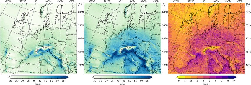
986                                 B. Poschlod et al.: Ten-year return levels of sub-daily extreme precipitation over Europe

small sample sizes (Delicado and Goria, 2008; Hosking et           ods are spatially interpolated over Germany resulting in grid
al., 1985; Kharin and Zwiers, 2000). We have also applied          cells of approximately 8 km. We rescale these grids linearly
maximum likelihood estimation (MLE). There, the median             to the 0.11◦ specifications of the CRCM5-LE.
return levels are almost equal to L-moments, but the vari-
ability within the 50 members is slightly larger due to more       3.1.2   Austria
unstable results at the edges of the ensemble. MLE is recom-
mended by Delicado and Goria (2008) for sample sizes of            The Austrian data set is publicly available for single grid cells
n ≥ 50, which is why we keep the fits based on the method          on a web portal by the Federal Ministry of Agriculture, Re-
of L-moments. The goodness of fit is assessed applying the         gions and Tourism (BMLRT, 2019). For the generation of
Anderson–Darling test with a 5 % significance level follow-        the return periods, the rain gauge data are supplemented by
ing Chen and Balakrishnan (1995). The goodness-of-fit test         a convective weather model in order to improve the density
with a 5 % significance level at 280 × 280 grid cells for 50       of observations (Kainz et al., 2007). Similarly to the German
members would yield 196 000 locations on average, where            dataset, a POT approach was applied. Details are reported in
the null hypothesis is erroneously rejected, also called the       BMLRT (2006). We linearly interpolate the Austrian data to
type I error or false positives (Ventura et al., 2004). Hence,     the 0.11◦ grid.
we apply the false discovery rate (FDR) (Benjamini and
Hochberg, 1995) following the approach of Wilks (2016),            3.1.3   Belgium
which adjusts the critical p value for statistical testing at
many locations. Less than 0.1 % of all fits are rejected for       Return periods of extreme precipitation in Belgium were cal-
all durations. The median values of µ, σ , and ξ , as well as      culated by van de Vyver (2012). Therefore, a spatial GEV
the respective standard deviation over the 50 members, are         model was applied considering multisite data. The GEV pa-
shown within the Supplementary materials. The 10-year re-          rameters are related to geographical and climatological co-
turn periods are calculated inverting Eq. (1). For the most ro-    variates through a regression relationship. The data are pro-
bust estimation at each grid cell, the median of the 50 return     vided by the Belgian Royal Meteorological Institute (RMI,
periods is chosen.                                                 2019; publicly available) for each commune. We interpolate
                                                                   the communal point data on the CRCM5-LE grid via ordi-
                                                                   nary kriging.
3     Observational rainfall return periods

The observational data are combined from many different            3.1.4   France
national precipitation data sets. This special effort had to
be made, since reanalysis products underrepresent extreme          Embedded in the framework of SHYPRE (Simulated Hy-
events due to the interpolation methods, especially in regions     drographs for flood Probability Estimation; Arnaud and
with a low measuring network density and for short-duration        Lavabre, 2002), Arnaud et al. (2008) apply an hourly
events at local scales (Hofstra et al., 2008). In order to com-    stochastic rainfall model to derive return periods of extreme
pare the national observational data to the climate model out-     precipitation in France. The data are not publicly available
put, areal precipitation data sets of observations are linearly    and were already provided with the CRCM5-LE grid specifi-
rescaled to the 0.11◦ CRCM5 grid. Point observations are           cations by Patrick Arnaud with permission of Météo-France.
spatially interpolated via ordinary kriging and aggregated to
the 0.11◦ grid of the CRCM5-LE. We describe the data pro-          3.1.5   Switzerland
cessing for each national data set in the following. Table 1
provides an overview of the applied observational data and         In Switzerland, return periods of hourly and 3, 6, and 12 h
how they were accessed.                                            precipitation are available at 67 rain gauges for the time pe-
                                                                   riod 1981 to 2019 (MeteoSwiss, 2016). They were calculated
                                                                   by fitting a GEV to seasonal maxima via Bayesian estima-
3.1     National data                                              tion. As 24 h return periods are not provided, we use the es-
3.1.1    Germany
                                                                   timates for daily extreme precipitation, which cover a time
                                                                   period from 1966 to 2015 at 337 sites. We apply an adjust-
The German weather service provides an estimation of rain-         ment factor of 1.14 to transfer the daily fixed-window return
fall return periods based on 5 min resolution gauge observa-       levels to 24 h moving-window levels as this relation has been
tions between 1951 and 2010 (DWD, 2019; publicly avail-            found to be rather stable (Barbero et al., 2019; Boughton and
able). The documentation of the data processing is given in        Jakob, 2008). Within the CRCM5-LE, we find a factor of
Malitz and Ertel (2015). A POT approach was chosen to              1.13 between daily and 24 h return periods, which confirms
sample extreme events. Events between May and September            this relationship. We interpolate the pointwise estimations of
were de-clustered to guarantee independent samples. After          the return levels to the CRCM5 grid applying ordinary krig-
fitting an exponential distribution, the calculated return peri-   ing.

Earth Syst. Sci. Data, 13, 983–1003, 2021                                            https://doi.org/10.5194/essd-13-983-2021
B. Poschlod et al.: Ten-year return levels of sub-daily extreme precipitation over Europe                                             987

Table 1. Overview of the national observational precipitation data sets in the same order as in Sect. 3.1.

  Country or state              Source                 DOI, URL, or ISBN                                         Access
  Germany                       DWD                    https://opendata.dwd.de/climate_environment/CDC/          Open access; last ac-
                                                       grids_germany/return_periods/precipitation/KOSTRA/        cess: 21 October 2019
                                                       KOSTRA_DWD_2010R/asc/
  Austria                       BMLRT                  https://ehyd.gv.at/                                       Open access; last ac-
                                                                                                                 cess: 22 October 2019
  Belgium                       RMI                    https://www.meteo.be/fr/climat/atlas-climatique/          Open access; last ac-
                                                       climat-dans-votre-commune                                 cess: 1 October 2019
  France                        Patrick Arnaud,        –                                                         No      open    access;
                                Météo-France                                                                     data were provided
                                                                                                                 by Patrick Arnaud
                                                                                                                 with permission of
                                                                                                                 Météo-France
  Switzerland                   MeteoSwiss             https://www.meteoswiss.admin.ch/home/climate/             Open access; last ac-
                                                       swiss-climate-in-detail/extreme-value-analyses/           cess: 11 October 2019
                                                       standard-period.html?station=int
  Norway (1–12 h)               Dyrrdal et al.         –                                                         No open access; data
                                (2015), NMI                                                                      were provided by NMI
                                                                                                                 for research only
  Norway (24 h)                 Lussana and Tveito     https://doi.org/10.5281/zenodo.845733                     Open access; last ac-
                                (2017)                                                                           cess: 11 January 2020
  Slovenia                      SEA                    http://meteo.arso.gov.si/met/sl/climate/tables/precip_    Open access; last ac-
                                                       return_periods_newer/                                     cess: 30 January 2020
  United Kingdom                Lewis et al.           https://doi.org/10.5285/d4ddc781-25f3-423a-bba0-          Open access; last ac-
                                (2019b)                747cc82dc6fa                                              cess: 23 January 2020
  Denmark                       Madsen et al.          –                                                         Single numbers for the
                                (2017)                                                                           whole country are given
                                                                                                                 in Sect. 3.1.9
  The Netherlands (1–12 h)      Beersma et al.         –                                                         Single numbers for the
                                (2018)                                                                           whole country are given
                                                                                                                 in Sect. 3.1.10
  The Netherlands (24 h)        KNMI                   https://data.knmi.nl/datasets/Rd1/5&Openaccess; last
                                                       access: 2 October 2019
  Sweden                        Olsson et al.          https://www.smhi.se/polopoly_fs/1.134304!/                Open access; last ac-
                                (2018)                 klimatologi_47_4.pdf                                      cess: 30 July 2020
  Finland (1 h)                 Aaltonen et al.        https://helda.helsinki.fi/bitstream/handle/10138/38381/   Open access; last ac-
                                (2008)                 SY_31_2008.pdf                                            cess: 30 July 2020
  Finland (6 and 24 h)          Venäläinen et al.      https://helda.helsinki.fi/bitstream/handle/10138/1138/    Open access; last ac-
                                (2007)                 Korjattu2007nro{%}204.pdf                                 cess: 30 July 2020
  Italy
  Basilicata                    Manfreda et al.        http://www.centrofunzionalebasilicata.it/it/pdf/          Open access; last ac-
                                (2015)                 pioggia_download.pdf                                      cess: 30 July 2020
  Calabria                      ARPACAL                http://www.cfd.calabria.it/index.php/dati-stazioni/       Open access; personal
                                                       dati-storici                                              registration needed;
                                                                                                                 last access: 30 January
                                                                                                                 2020
  Friuli Venezia Giulia         ARPAFVG                https://www.osmer.fvg.it/clima.php?ln=                    Open access; last ac-
                                                                                                                 cess: 10 January 2020
  Marche                        PCRM                   http://app.protezionecivile.marche.it/sol/indexjs.sol?    Open access; user ac-
                                                       lang=en&Ok=1                                              count necessary; last
                                                                                                                 access: 20 December
                                                                                                                 2019
  Piedmont                      ARPAP                  https://www.arpa.piemonte.it/rischinaturali/              Open access; Java ap-
                                                       accesso-ai-dati/annali_meteoidrologici/                   plication; last access:
                                                       annali-meteo-idro/banca-dati-meteorologica.html           20 January 2020

https://doi.org/10.5194/essd-13-983-2021                                                    Earth Syst. Sci. Data, 13, 983–1003, 2021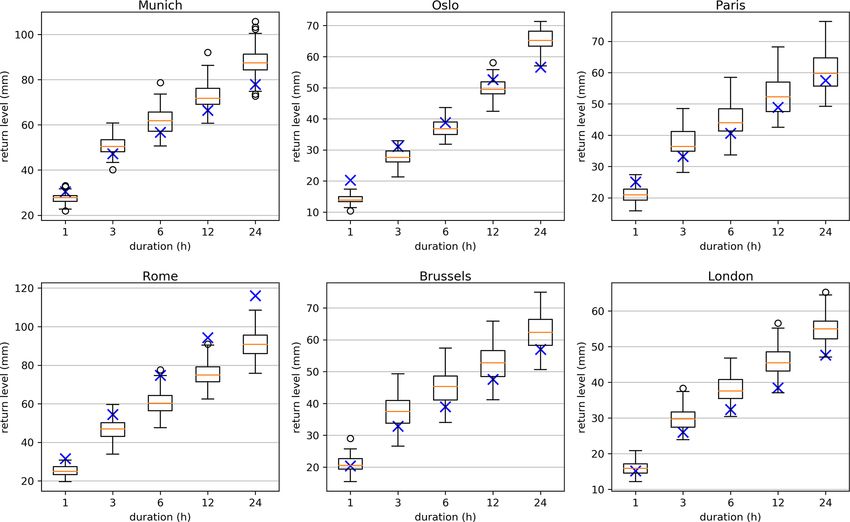
988                                    B. Poschlod et al.: Ten-year return levels of sub-daily extreme precipitation over Europe

Table 1. Continued.

        Country or state   Source                DOI, URL or ISBN                                           Access
        Tuscany            RT                    http://www.sir.toscana.it/consistenza-rete                 Open access; last
                                                                                                            access: 11 December
                                                                                                            2019
        Trento             Meteotrentino         http://storico.meteotrentino.it/web.htm                    Open access; last
                                                                                                            access: 21 December
                                                                                                            2019
        Umbria             Morbidelli et al.     ISBN (EAN): 978-88-6074-805-8                              –
                           (2016)
        Aosta Valley       CFRAVA                https://cf.regione.vda.it/portale_dati.php                 Open access; last ac-
                                                                                                            cess: 5 January 2020
        Lazio              CFRRL                 http://www.idrografico.regione.lazio.it/std_page.          Open access; last ac-
                                                 aspx-Page=curve_pp.htm                                     cess: 8 January 2020
        Liguria            ARPAL                 https://www.arpal.liguria.it/contenuti_statici/clima/      Open access; last ac-
                                                 atlante/Atlante_climatico_della_Liguria.pdf                cess: 30 July 2020
        Veneto             ARPAV                 https://www.arpa.veneto.it/bollettini/storico/precmax/     Open access; last ac-
                                                                                                            cess: 3 January 2020
        Lombardy           De Michele et al.     http://idro.arpalombardia.it/manual/lspp.pdf               Open access; last ac-
                           (2005)                                                                           cess: 30 July 2020
        Molise             RM (2001)             http://regione.molise.it/llpp/pdfs/b-1-2.pdf               Open access; last ac-
                                                                                                            cess: 30 July 2020
        Spain              SMG                   https://meteo.unican.es/tds5/catalog/pr_Spain02_v5.0_      Open access; last ac-
                                                 011rot/catalog.html?dataset=pr_Spain02_v5.0_011rot/        cess: 11 November
                                                 Spain02_v5.0_DD_011rot_aa3d_pr.nc                          2019
        Portugal           IPMA                  https://www.ipma.pt/en/produtoseservicos/index.jsp?        Open access; last ac-
                                                 page=dataset.pt02.xml                                      cess: 12 October 2019
        Poland             Berezwoski et al.     https://doi.org/10.4121/uuid:e939aec0-bdd1-440f-           Open access; last ac-
                           (2015)                bd1e-c49ff10d0a07                                          cess: 21 November
                                                                                                            2019

3.1.6    Norway                                                         ξ = 0). The time periods differ for each site. We interpolate
                                                                        the return levels to the 0.11◦ grid via ordinary kriging.
Dyrrdal et al. (2015) generate a spatially coherent map of ex-
treme hourly precipitation return levels in Norway. They link
GEV distributions with latent Gaussian fields in a Bayesian             3.1.8    United Kingdom (without Northern Ireland)
hierarchical model to overcome the sparse observational net-
work. The precipitation gauges only operate during an ex-               For the United Kingdom, we use the gridded estimates
tended summer season, whereas the highest 12 and 24 h rain-             of hourly areal rainfall for Great Britain (CEH-GEAR1hr;
fall sums occur during fall and winter in western Norway.               Lewis et al., 2019b; publicly available), which covers a time
Due to this limitation, the data have to be classified as ex-           period of 1990 to 2014 in a 1 km spatial resolution. For every
perimental. Hence, for 24 h return levels, we use the daily             grid cell and duration, we sample the annual maxima, fit the
gridded precipitation data set seNorge2 at a 1 km resolution            GEV, and calculate the return levels. Then, we aggregate the
(Lussana and Tveito, 2017 – publicly available; Lussana et              areal rainfall return levels to the 0.11◦ grid.
al., 2018), which covers the time period from 1957 to 2019.
We fit the GEV to the annual maxima of each 1 km grid cell
                                                                        3.1.9    Denmark
and apply the adjustment factor of 1.14 to transfer the daily
estimates to moving windows of 24 h. The resulting return               For the Danish climate, the rainfall return levels are assumed
levels are then linearly interpolated to the 0.11◦ grid.                to be almost constant with very low variability across the
                                                                        whole country (Madsen et al., 2017). The authors used data
3.1.7    Slovenia                                                       of 83 rain gauges with a 1 min resolution covering the period
                                                                        1979 to 2012 with more than 10 years of observations. For
The Slovenian Environment Agency provides rainfall return               the extreme value analysis, a partial duration series model
periods at 63 gauges (SEA, 2020; publicly available), which             is applied to estimate the intensity–duration–frequency rela-
they derived by fitting a Gumbel distribution (see Eq. 1 with           tionships of extreme precipitation. We use their average val-

Earth Syst. Sci. Data, 13, 983–1003, 2021                                                     https://doi.org/10.5194/essd-13-983-2021
B. Poschlod et al.: Ten-year return levels of sub-daily extreme precipitation over Europe 989
ues of 24.9 mm (33.3, 40.2, 46.7, 55.3 mm) as 10-year return 3.1.13 Italy
levels for hourly (3, 6, 12, 24 h) durations.
In Italy, meteorological observations are the responsibility of
the provincial administration. The data availability, the data
3.1.10 The Netherlands format, and the available products differ within all 21 re-
As for Denmark, the return levels show very low variability gional authorities. A good overview of this issue is given in
in the Netherlands, which is why the KNMI provides sin- Libertino et al. (2018), who also analyse the combined prod-
gle values for the whole country (Beersma et al., 2018). The uct, Italian Rainfall Extremes Database. However, the au-
10-year return levels amount to 31 mm h−1 , 39.8 mm (3 h)−1 , thors are not allowed to pass on this database, unless the per-
46.0 mm (6 h)−1 , and 52.9 mm (12 h)−1 . As no estimation for mission of all individual provincial administrations has been
24 h return levels is provided, we use daily precipitation sums obtained. We therefore focus on data, which are available,
of the 1 km resolution gridded data set between 1951 and and gathered information for 14 provinces. Annual max-
2010 (KNMI, 2019; publicly available). The data are based ima for rain gauges are provided for Basilicata (Manfreda et
on 300 measurement stations and interpolated via ordinary al., 2015), Calabria (ARPACAL, 2020; personal registration
kriging. After extracting the annual maxima, we fit the GEV needed), Friuli Venezia Giulia (ARPAFVG, 2020), Marche
and rescale the resulting return level of daily precipitation to (PCRM, 2019; user account necessary), Piedmont (ARPAP,
the 0.11◦ grid. Furthermore, we apply the adjustment factor 2020; Java application of database has to be downloaded and
of 1.14 to transfer the return level to a 24 h estimate. run), Tuscany (RT, 2019), Trento (Meteotrentino, 2019), Um-
bria (Morbidelli et al., 2016), and Aosta Valley (CFRAVA,
2020). We fitted the GEV and calculated the 10-year return
3.1.11 Sweden
levels. Rainfall return levels are directly available for sta-
In Sweden, the variability in return periods of extreme pre- tions in Lazio (CFRRL, 2018), Liguria (ARPAL, 2013), and
cipitation is also assumed to be very low. Olsson et al. (2018) Veneto (ARPAV, 2020). Fitted parameters for the LSPP (linea
provide tables of hourly and 3, 6, and 12 h return levels for segnalatrice di probabilità pluviometrica) model are given for
four regions of Sweden. The estimations are based on over rain gauges in Lombardy by de Michele et al. (2005), which
120 rain gauges covering the period 1996 to 2017. For each can be used to derive rainfall intensities for the 10-year return
of the four regions, all rain gauge data were concatenated period. For the stations in the region of Molise, fitted param-
into one single time series. A POT approach was carried out, eters for an exponential model are provided (RM, 2001). All
and the generalized Pareto distribution (GPD) was fitted via derived point data of return levels were interpolated applying
maximum likelihood estimation. The domain of the CRCM5- ordinary kriging.
LE covers only the middle, south-eastern, and south-western
Swedish sub-regions. The 24 h duration is not available, and 3.1.14 Spain
we therefore apply an extrapolated value for the three re-
gions, which is adapted to the values of the neighbouring For Spain, we have only gathered information about daily
countries Finland and Denmark. rainfall return levels. Herrera et al. (2012) have developed
a gridded data set of daily precipitation sums based on 2756
measurement stations for the period 1950 to 2003. They used
3.1.12 Finland
a two-stage kriging approach to interpolate the data. Due to
Within a project about short-duration rainfall extremes in ur- the dense station network, extreme precipitation events are
ban areas, radar measurements over the whole of Finland be- accurately reproduced in contrast to typical reanalysis data
tween 2000 and 2005 have been used to estimate the hourly sets. The data are publicly available (SMG, 2019). We ex-
return level of 10-year rainfall (Aaltonen et al., 2008). The tracted the annual maxima, fitted the GEV, and applied the
radar measurements of the whole country were pooled to en- adjustment factor of 1.14 to transfer the daily data to 24 h
large the database for extreme value analysis. The hourly moving-window estimations. Then we rescaled the gridded
10-year return level amounts to 22.9 mm h−1 for the whole data to the specifications of the 0.11◦ CRCM5 grid.
country. For longer durations of 6 and 24 h, Venäläinen et
al. (2007) have calculated return levels for different sites in 3.1.15 Portugal
Finland. As for Denmark, we take one average value for the
whole country from the stations, which are covered by the Following the same approach as the Spanish data set, Belo-
CRCM5-LE domain. For 3 and 12 h estimates we interpo- Pereira et al. (2011) have created grid data of daily precip-
late according to the values of the neighbouring countries itation. The data set is based on 806 stations, and therefore
Sweden and Denmark. The final countrywide return levels the dense station network again ensures an accurate repro-
amount to 22.9 mm (27.0, 34.0, 44.0, 53.1 mm) as 10-year duction of extremes after the interpolation process. Data are
return levels for hourly (3, 6, 12, 24 h) durations. available at IPMA (2019; publicly available). We used the
same process as for the Spanish data to estimate 24 h return
levels.
https://doi.org/10.5194/essd-13-983-2021 Earth Syst. Sci. Data, 13, 983–1003, 2021990 B. Poschlod et al.: Ten-year return levels of sub-daily extreme precipitation over Europe
3.1.16 Poland store one file with five columns containing the return level
based on the median of the 50-member CRCM5-LE and the
Berezwoski et al. (2016) applied the interpolation by Herrera 5 % quantile and the 95 % quantile of the ensemble at each
et al. (2012) on up to 816 meteorological station data for the grid cell as well as the geographical coordinates. We use
time period of 1951 to 2013. The data are publicly available this format because of a possible application within a non-
(Berezwoski et al., 2015). We used the same process as for scientific environment, whereas within climate science, the
the Spanish data to estimate 24 h return levels. NetCDF format is widely used. Figure 1 shows the rainfall
intensity for hourly and 12 h precipitation return levels for
3.2 Post-processing for the comparison to areal data the European domain based on the median of the 50-member
CRCM5-LE. Though covering the whole year, Fig. 1 can
Most of the observational data sets are based on point mea- be compared to the 10-year return levels of nine RCM se-
surements, whereas the climate model simulates areal esti- tups of the EURO-CORDEX ensemble, which were calcu-
mates of precipitation. In order to improve the comparability lated for summertime precipitation only (Berg et al., 2019).
of these two kinds of data, areal reduction factors (ARFs) We chose the same colour scaling for better comparability.
are often applied to the point measurements (Wilson, 1990). The median return levels of the CRCM5-LE show a more
ARFs are empirically derived factors and are dependent on homogeneous regional distribution with less scattering than
the temporal and spatial resolution as well as on the local the single RCM members in Berg et al. (2019). Also, single
climate (Sunyer et al., 2016). In addition to the difference in members of the CRCM5-LE show this smooth regional dis-
space, we need to apply a correction to the hourly data, as tribution, but the use of the median of 50 SMILE members
the observations are based on hourly maxima with moving enhances this behaviour, as it filters out the internal variabil-
windows, whereas the hourly data of the climate model are ity in the climate system within individual 30-year periods.
constrained to the fixed window between full hours. For the hourly return levels, the combination of CanESM2
To account for different regional climates, we apply dif- and CRCM5 shows relatively high intensities such as the two
fering ARFs. In Finland, Norway, Sweden, Denmark, the most intense model setups HIRHAM5–ECEARTH-r03 and
United Kingdom, Denmark, the Netherlands, Belgium, Ger- REMO2009–MPI-ESM-RL in Berg et al. (2019). However,
many, and Switzerland, we apply the ARF from Berg et the spatial pattern differs, as the CRCM5-LE produces lower
al. (2019) for 3 (ARF3 h = 1.06), 6 (ARF6 h = 1.02), and hourly rainfall intensities in the eastern part of the study area
12 h (ARF12 h = 1.01) durations. For the 24 h data, no ad- and shows a higher sensitivity to the topography of the Alps.
justment is needed. For the hourly resolution we apply the In the central Alpine areas, the CRCM5-LE simulates very
ARF1 h = 1.279 from Sunyer et al. (2016) following Wilson low hourly rainfall intensities of 6 to 15 mm h−1 . The highest
(1990). rainfall intensities are simulated south of the Alps and at the
In Austria and Slovenia, we use the ARFs by Breinl et Adriatic coast.
al. (2020), which amount to 1.30 (1.20, 1.13, 1.09, 1.06) for For the 12 h duration, these areas also show the highest
hourly (3, 6, 12, 24 h, respectively) duration. In the Italian median rainfall intensities, with the Norwegian west coast
provinces, the reduction factors by Mineo et al. (2018) are and the Atlantic coast of northern Portugal and Spain also
applied. These show a stronger reduction for shorter dura- exhibiting high values. The lowest 12 h return levels are pro-
tions (ARF1 h = 1.52; ARF3 h = 1.22; ARF6 h = 1.07). For duced for the south-west and the north of the study area
12 and 24 h durations, Mineo et al. (2018) do not propose (northern Africa, UK, Scandinavia, and north-eastern Eu-
any reduction. As the areal correction is already implemented rope). The 12 h 10-year return levels based on the median
within the SHYPRE process chain of the French data, we of the CRCM5-LE are similar to all nine RCM-GCM com-
only apply temporal correction factors of 1.03, 1.02, and binations of Berg et al. (2019) in terms of spatial patterns as
1.01 for hourly and 3 and 6 h durations following Berg et well as rainfall intensities. Hence, we argue that the differ-
al. (2019). These temporal correction factors are also added ences between the parametrization of convection induces the
to the ARFs of Wilson (1990), Breinl et al. (2020), and Mi- big deviations within the hourly return levels, because for this
neo et al. (2018). An overview of the applied ARFs is given duration convection is the main driver of extreme precipita-
in Table 2. tion in large parts of Europe (Berg et al., 2013; Coppola et al.,
For the combination of the overlapping national data sets, 2020; Lenderink and Meijgaard, 2008; Kendon et al., 2014).
the mean of the two overlapping data sets is calculated. In order to compare the return levels of the CRCM5-LE to
observational data, we present both data sets as well as the
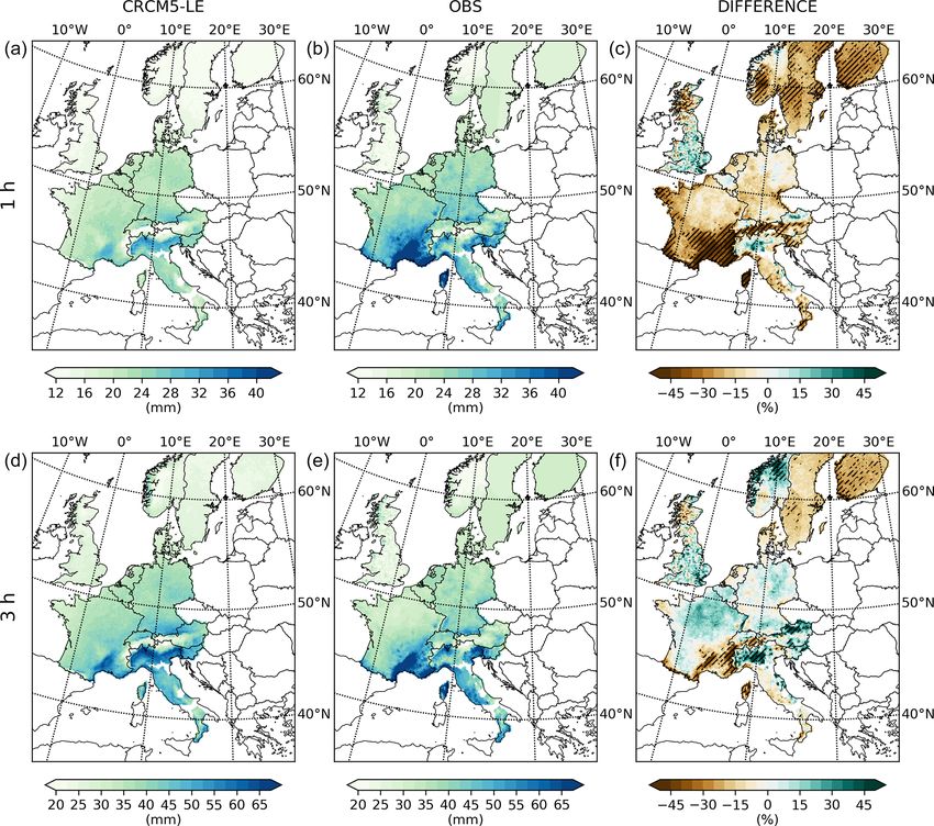
4 Results percentage deviation in Figs. 2–4 for all durations.
The combined observational datasets (see Figs. 2–4) show
The median at each grid point of the 10-year return lev- quite smooth transitions between most of the different data
els of hourly and 3, 6, 12, and 24 h precipitation of the 50 sources and methods. The biggest deviation is found at the
CRCM5-LE members is generated and stored as comma- border of Norway and Sweden for hourly to 12 h durations
separated text files (Poschlod 2020). For each duration we (see Figs. 2 and 3), as the estimate of the rainfall return level
Earth Syst. Sci. Data, 13, 983–1003, 2021 https://doi.org/10.5194/essd-13-983-2021B. Poschlod et al.: Ten-year return levels of sub-daily extreme precipitation over Europe 991
Table 2. Applied areal reduction factors (ARFs) including temporal correction.
ARF1 h ARF3 h ARF6 h ARF12 h ARF24 h
Germany 1.32 1.06 1.02 1.01 1
Austria 1.34 1.24 1.14 1.09 1.06
Belgium 1.32 1.06 1.02 1.01 1
France∗ 1.03 1.02 1.01 1 1
Switzerland 1.32 1.06 1.02 1.01 1
Norway 1.32 1.06 1.02 1.01 1
Slovenia 1.34 1.24 1.14 1.09 1.06
United Kingdom 1.32 1.06 1.02 1.01 1
Denmark 1.32 1.06 1.02 1.01 1
The Netherlands 1.32 1.06 1.02 1.01 1
Sweden 1.32 1.06 1.02 1.01 1
Finland 1.32 1.06 1.02 1.01 1
Italy 1.56 1.24 1.08 1 1
Spain – – – – 1
Portugal – – – – 1
Poland – – – – 1
∗ In France the areal reduction is implemented within the SHYPRE process chain. Only temporal
correction factors are added.
Figure 1. The 10-year return levels of hourly (a) and 12 h (b) precipitation over Europe based on the median of the 50-member CRCM5-LE.
for western Sweden by Olsson et al. (2018) is a lot higher deviations emphasize the need for homogeneous data sets of
than the estimate by Dyrrdal et al. (2015) for eastern Nor- extreme precipitation.
way. This is due to the sparse sampling of observations and As the 50 members of the CRCM5-LE also provide a
differing approaches to derive return levels (see Sect. 3.1). range of equally probable estimations of return levels, we
We also find slight deviations for the Netherlands, where the hatch areas where the observations are not within the range
return levels by Beersma et al. (2018) are higher than the of the regional climate model ensemble. The rainfall in-
surrounding levels for northern Belgium and western Ger- tensity of the observational data set is within the range of
many. For the shorter durations of hourly and 3 h return lev- the climate-model-generated intensities in 60 % (77 %, 78 %,
els (see Fig. 2), deviations occur at the border between Italy 83 %, 78 %) of the area for hourly (3, 6, 12, 24 h) durations
and France as well as between Italy and Switzerland. This is (see Figs. 2–4). This fraction of areas gradually increases
due to the higher ARF applied in Italy (see Sect. 3.2). These between hourly and 12 h durations, whereas it slightly de-
https://doi.org/10.5194/essd-13-983-2021 Earth Syst. Sci. Data, 13, 983–1003, 2021992 B. Poschlod et al.: Ten-year return levels of sub-daily extreme precipitation over Europe Figure 2. The 10-year return levels of hourly (a–c) and 3 h (d–f) precipitation over parts of Europe. The CRCM5-LE data (a, d) are compared to an observational data set (b, e), and the percentage deviation (c, f) is shown. Areas where the observations are not in the range of the CRCM5-LE are hatched. creases for the 24 h duration. For the 24 h return period, data crease to −1.0 %, −0.5 %, and +0.1 % (see Figs. 2 and 3). for the Iberian Peninsula and Poland were added, whereas The high intensities of southern France, southern Switzer- no data for these countries were available for the hourly to land, and parts of Italy are underestimated (see Figs. 2 and 3). 12 h evaluation. Without these additional data sets, the frac- Also in Sweden and Finland the observational data sets report tion of areas where 24 h observational return levels are within higher rainfall intensities. For the 24 h aggregation, the bias the CRCM5-LE return levels would amount to 80 %. In addi- amounts to +8.2 % (see Fig. 4). The CRCM5 overestimates tion, in the Netherlands, Switzerland, and Norway, different 24 h rainfall intensities in western Norway and at the Atlantic databases are used for the estimations of the return levels of coast of the northern Iberian Peninsula, which is why the ob- hourly to 12 h durations and the 24 h duration (see Sect. 3). servations are not in the range of the 50 CRCM-LE members The hourly intensities are generally underestimated by the (see Fig. 4). CRCM5-LE except for England and Wales, northern Italy, We calculate Spearman’s rank correlation coefficient ρ as northern Austria, and the northern part of Norway, resulting a measure to compare the spatial patterns. For the median in an areal average bias of −16.3 % (see Fig. 2). There is of the return levels of the CRCM5-LE and the observational also an area-wide underestimation in the Mediterranean as data, the coefficient amounts to 0.83 (0.81, 0.76, 0.78, 0.83, well as in Scandinavia in all 50 members of the large en- respectively) of the area for hourly (3, 6, 12, 24 h, respec- semble, which is why the observations are not in the range tively) durations. These values confirm the visual impression of the CRCM5-LE for large parts of these areas (see Fig. 2). of a high spatial pattern correlation when comparing both For durations of 3 to 12 h, the biases over the whole area de- data sets (see Figs. 2–4). Earth Syst. Sci. Data, 13, 983–1003, 2021 https://doi.org/10.5194/essd-13-983-2021
B. Poschlod et al.: Ten-year return levels of sub-daily extreme precipitation over Europe                                             993

Figure 3. The 10-year return levels of 6 (a–c) and 12 h (d–f) precipitation over parts of Europe. The CRCM5- LE data (a, d) are compared
to an observational data set (b, e), and the percentage deviation (c, f) is shown. Areas where the observations are not in the range of the
CRCM5-LE are hatched.

5   Discussion                                                          5.1   Uncertainties in observational data

Generally, the overall low bias of the return levels based on           Due to differing methods, temporal resolutions of the rain
climate model data as well as the high spatial correlation be-          gauges, available time periods, and areal coverage, we do
tween the observational and modelled return levels proves               not regard the combined observational data set as “truth”
that the CRCM5-LE is able to capture the features of the het-           but as the largest possible comparison product, which is di-
erogeneous set of drivers which govern the European climate             rectly based on hourly observations. The uncertainties within
of heavy and extreme precipitation.                                     these data are caused by different sources. First, the rain
   Especially for countries without any sub-daily precipita-            gauge measurements systematically underestimate precipita-
tion measurement, the data set based on climate model sim-              tion due to splashing raindrops, wetting of the funnel sur-
ulations can provide valuable estimations. But also for coun-           face, evaporation from the funnel, and wind effects (Førland
tries offering return levels of extreme sub-daily precipitation,        et al., 1996; Richter, 1995; Westra et al., 2014). The choice
our results show that the sparse observational network can              of the sampling approach as well as the choice of the extreme
be supported by climate model simulations. Accordingly, the             value distribution leads to differing estimations of return lev-
Austrian return level data (Sect. 3.1) are supplemented by a            els (Lazoglou and Anagnostopoulou, 2017). Also, the fitting
convective-permitting weather model (Kainz et al., 2007).               of the parameters of the respective extreme value distribution
                                                                        to the extreme-precipitation samples induces additional un-
                                                                        certainty (Muller et al., 2009). As described in Sect. 3.1, the

https://doi.org/10.5194/essd-13-983-2021                                                 Earth Syst. Sci. Data, 13, 983–1003, 2021
994 B. Poschlod et al.: Ten-year return levels of sub-daily extreme precipitation over Europe Figure 4. The 10-year return levels of 24 h precipitation over parts of Europe. The CRCM5-LE data (a) are compared to an observational data set (b), and the percentage deviation (c) is shown. Areas where the observations are not in the range of the CRCM5-LE are hatched. applied EVT approaches differ for the national data sets. La- able (Zolina et al., 2014). Therefore, the representativeness zoglou and Anagnostopoulou (2017) have shown that the es- of single-point observations is limited. timations of 50-year return levels of daily precipitation at 10 Transferring these rather uncertain point-scale different Mediterranean stations differ by between 5 % and observation-based data to areal estimates can be car- 15 % according to the application of GEV or GPD and three ried out with various spatial interpolation methods such as different fitting methods. inverse distance weighting; multivariate splines, machine The national data sets of Norway and Germany do not re- learning approaches; or different versions of kriging, where fer to all seasons but cover only summertime events (Dyrrdal auxiliary geographical or climatological covariates can be et al., 2015; Malitz and Ertel, 2015). The available time pe- added via regression fields (e.g. Malitz and Ertel, 2015; van riods of observations not only differ for all countries but also de Vyver, 2012). In combination with low spatial coverage differ within the countries, as new rain gauges were installed of the rain gauges (Isotta et al., 2014), this step induces over time and other measurement stations were discarded. additional methodological uncertainties. The regionalization Short time periods increase the uncertainties in the param- of extreme precipitation is subject to a wide field of research, eter fits of the extreme value distribution (Cai and Hames, where many sophisticated methods are applied that show 2011). Additionally, extreme precipitation, especially when different interpolation results (Hu et al., 2019). Because for caused by convectional processes, is spatially highly vari- most countries only the return level itself and not the time Earth Syst. Sci. Data, 13, 983–1003, 2021 https://doi.org/10.5194/essd-13-983-2021
B. Poschlod et al.: Ten-year return levels of sub-daily extreme precipitation over Europe                                      995

series of rainfall is provided, we applied ordinary kriging to      respectively, which equals a percentage range of −14 % to
regionalize the observational point data.                           +17 %. This range is quite stable for other durations as well
   The linear scaling to the 0.11◦ CRCM5-LE grid was ap-            (−15 % to +18 % for hourly and −15 % to +14 % for 6,
plied to the national data, which are provided as areal esti-       −14 % to +17 % for 12, and −13 % to +17 % for 24 h du-
mates with different spatial resolutions. The aggregation and       rations). Thereby, the overall variability is mainly caused by
linear scaling to the spatial resolution of 0.11◦ smooths ex-       natural variability in the rainfall intensity. The spatial pat-
treme values of single grid cells.                                  terns of the minimum and maximum estimates show high
   The last step to make observation data and climate model         agreement with a Spearman’s rank correlation coefficient of
data comparable features the application of the areal reduc-        ρ = 0.91. Hence, we conclude that the application of annual
tion factor (ARF). The ARFs are derived empirically and             maxima of 30-year periods and EVT can filter out the spatial
therefore differ between different studies, which also causes       variability in single extreme events, but the estimates of 10-
uncertainty (Berg et al., 2019; Sunyer et al., 2016; Wilson,        year return levels are still governed by the natural variability
1990).                                                              within the 30-year periods.
   Junghänel et al. (2017) estimate a tolerance range of               For a local-scale visualization, we provide the range of the
±15 % for 10-year return levels of the German national data         CRCM5-LE return levels as well as the observational return
(Sect. 3.1.1).                                                      levels for all considered durations at six different European
   Even though the combined observational data set is subject       cities (see Fig. 6). Oslo, London, Brussels, Paris, Munich,
to different limitations and uncertainties, it is a necessary ap-   and Rome show different climates and distances to the ocean.
proach not only to evaluate the return levels of climate mod-       We also include the city of Rome as an example of where
els locally or countrywide but also to perform validation at an     the observational data are not within the range of the climate
(almost) continental scale. To our knowledge, such an assess-       model simulations. We find that the absolute range of natural
ment has not been carried out before. The confidence level in       variability is dependent on the intensity of rainfall, which is
this validation varies by country depending on the underlying       also visible in the standard deviation in Fig. 5. We argue that
rainfall database and the procedure of the return level calcu-      convective processes are more affected by natural variabil-
lation, which has been described in Sect. 3. The obvious devi-      ity and, therefore, the return levels in Rome and Paris show
ations in our homogenized observational return level product        greater variability than in Oslo or London.
at the country borders between Norway and Sweden and be-               Due to the application of a SMILE, natural variability in
tween Italy, France, and Switzerland as well as between the         return levels of extreme rainfall can now be quantitatively
Netherlands, Germany, and Belgium (as described in Sect. 4)         assessed at local, regional, and continental scales. Before, it
show that the validation in these regions is subject to major       had been included within uncertainty estimations of obser-
uncertainties for hourly to 12 h durations. On the other hand,      vational return levels as an additional source of uncertainty
the good fit and the preservation of topographic features at        (Junghänel et al., 2017) but was only estimated rather arbi-
the borders of Germany, Denmark, Belgium, France, Aus-              trarily.
tria, Switzerland, and Slovenia support the confidence level
in the validation for these regions. For the 24 h duration we       5.3   Limitations of the CRCM5-LE
find no major deviations along the country borders, which
increases the confidence in this return level duration.             In general, the results of the CRCM5-LE are governed by
                                                                    model uncertainty, as the ensemble only features one com-
5.2   Natural variability within the CRCM5-LE
                                                                    bination of GCM and RCM. Different model combinations
                                                                    or even modifications of the dynamics, physics, and struc-
Extreme precipitation events show a high variability due to         ture of the same climate models would yield different return
the natural variability in the climate system (Aalbers et al.,      level estimates. The results of the study by Berg et al. (2019)
2018). By the application of a 50-member SMILE, we as-              suggest that the influence on the return level estimates of
sume the range of natural variability in extreme rainfall to        the RCM is significantly greater than that of the atmospheric
be represented by the ensemble (Deser et al., 2012; Hawkins         forcing by the GCM.
and Sutton, 2009; von Trentini et al., 2019). In consequence,          The return levels simulated by the CRCM5-LE are lim-
while all 50 members are forced by the same emissions and           ited by the spatial resolution of the model setup, by the
are simulated by the same model structure and physics, the          temporal resolution of the stored precipitation output, and
resulting return levels differ from each other.                     by the non-explicit calculation of convectional precipitation
   In order to visualize this range, we show the standard de-       using parametrization schemes. Short-duration rainfall ex-
viation, as well as the 5 % and 95 % quantiles of all 50 mem-       tremes over Europe are mainly governed by convectional
bers at each grid cell representing the 10-year return level of     processes, which can only be resolved by regional climate
3 h precipitation (Fig. 5). The standard deviation amounts to       models with explicit convection schemes, i.e. spatial resolu-
3.33 mm as the areal average. The 5 %- and 95 %-quantile            tions of 4 km or less (Tabari et al., 2016). Prein et al. (2015)
return levels differ by −4.7 and +5.8 mm from the median,           have shown that improved spatial resolution also leads to

https://doi.org/10.5194/essd-13-983-2021                                            Earth Syst. Sci. Data, 13, 983–1003, 2021
996 B. Poschlod et al.: Ten-year return levels of sub-daily extreme precipitation over Europe Figure 5. The 5 % quantile (a), 95 % quantile, (b) and standard deviation (c) of the 50 CRCM5-LE members for 10-year return levels of 3 h precipitation over Europe. Figure 6. The range of the 10-year return levels of the CRCM5-LE at six cities is shown as box plots, where the median corresponds to the orange line. The boxes are defined by the first and third quartiles. Outliers exceed the first or third quartile plus 1.5 times the interquartile range. They are depicted as black circles. The observational return levels are marked as blue crosses. better reproduction of convectional rainfall. Several studies in south-western Germany or the Apennines in central Italy have reported that the application of convection-permitting (see Fig. 3). The CRCM5-LE simulates the areas of high- models (CPMs) improves the reproduction of heavy-rainfall intensity orographically enhanced precipitation one to two events over Europe (Berthou et al., 2020; Kendon et al., 2014, grid cells further to the west than the observational data set. 2017; Poschlod et al., 2018). In addition to the benefit of ex- These deviations do not affect the bias as a quality measure, plicitly calculating convection, complex topography is better as the areal average intensity is reproduced, but the location resolved with a better spatial resolution. The 0.11◦ resolu- is not correctly estimated. However, the centred Spearman tion of the CRCM5-LE equals around 12.5 km, which leads product-moment coefficient includes these local deviations. to systematic shifts in the location of high orographic precip- We argue that a higher spatial resolution would be able to itation. This phenomenon is visible for steep mountainous lower these errors. slopes with a westward exposition, such as the Black Forest Earth Syst. Sci. Data, 13, 983–1003, 2021 https://doi.org/10.5194/essd-13-983-2021
You can also read