FALL3D-8.0: a computational model for atmospheric transport and deposition of particles, aerosols and radionuclides - Part 2: Model validation
←
→
Page content transcription
If your browser does not render page correctly, please read the page content below
Geosci. Model Dev., 14, 409–436, 2021
https://doi.org/10.5194/gmd-14-409-2021
© Author(s) 2021. This work is distributed under
the Creative Commons Attribution 4.0 License.

FALL3D-8.0: a computational model for atmospheric transport and
deposition of particles, aerosols and radionuclides – Part 2:
Model validation
Andrew T. Prata1 , Leonardo Mingari1 , Arnau Folch1 , Giovanni Macedonio2 , and Antonio Costa3
1 Barcelona  Supercomputing Center (BSC), Barcelona, Spain
2 Istituto Nazionale di Geofisica e Vulcanologia, Osservatorio Vesuviano, Naples, Italy
3 Istituto Nazionale di Geofisica e Vulcanologia, Sezione di Bologna, Bologna, Italy

Correspondence: Andrew T. Prata (andrew.prata@bsc.es)

Received: 27 May 2020 – Discussion started: 17 June 2020
Revised: 4 November 2020 – Accepted: 19 November 2020 – Published: 25 January 2021

Abstract. This paper presents model validation results for        and FMS scores greater than 0.40 indicate acceptable agree-
the latest version release of the FALL3D atmospheric trans-       ment with satellite retrievals of volcanic ash and SO2 . In ad-
port model. The code has been redesigned from scratch to          dition, we show very good agreement, across several orders
incorporate different categories of species and to overcome       of magnitude, between the model and observations for the
legacy issues that precluded its preparation towards extreme-     2013 Mt. Etna and 1986 Chernobyl case studies. Our results,
scale computing. The model validation is based on the new         along with the validation datasets provided in the publicly
FALL3D-8.0 test suite, which comprises a set of four real         available test suite, form the basis for future improvements
case studies that encapsulate the major features of the model;    to FALL3D (version 8 or later) and also allow for model in-
namely, the simulation of long-range fine volcanic ash dis-       tercomparison studies.
persal, volcanic SO2 dispersal, tephra fallout deposits and
the dispersal and deposition of radionuclides. The first two
test suite cases (i.e. the June 2011 Puyehue-Cordón Caulle
ash cloud and the June 2019 Raikoke SO2 cloud) are val-           1   Introduction
idated against geostationary satellite retrievals and demon-
strate the new FALL3D data insertion scheme. The metrics          FALL3D-8.0 is the latest major version release of FALL3D
used to validate the volcanic ash and SO2 simulations are the     (Costa et al., 2006; Folch et al., 2009), an open-source code
structure, amplitude and location (SAL) metric and the figure     with a 15-year+ track record and a growing number of
of merit in space (FMS). The other two test suite cases (i.e.     users in the volcanological and atmospheric science com-
the February 2013 Mt. Etna ash cloud and associated tephra        munities. A companion paper (Folch et al., 2020) details
fallout deposit, and the dispersal of radionuclides resulting     the physics and the novel numerical implementation of the
from the 1986 Chernobyl nuclear accident) are validated with      code, which has been redesigned and rewritten from scratch
scattered ground-based observations of deposit load and lo-       in the framework of the EU Centre of Excellence for Ex-
cal particle grain size distributions and with measurements       ascale in Solid Earth (ChEESE). From the point of view
from the Radioactivity Environmental Monitoring database.         of model physics, a relevant improvement in the new ver-
For validation of tephra deposit loads and radionuclides, we      sion (v8.x) has been the generalisation of the code to deal
use two variants of the normalised root-mean-square error         with atmospheric species other than tephra including other
metric. We find that FALL3D-8.0 simulations initialised with      types of particles (e.g. mineral dust), gases and radionuclides
data insertion consistently improve agreement with satellite      (see Table 3 in Folch et al., 2020, for details). These differ-
retrievals at all lead times up to 48 h for both volcanic ash     ent categories and subcategories of species can be simulated
and SO2 simulations. In general, SAL scores lower than 1.5        using independent sets of bins that allow for dedicated pa-

Published by Copernicus Publications on behalf of the European Geosciences Union.
410                                                                                      A. T. Prata et al.: FALL3D-8.0 – Part 2

rameterisations for physics, emissions (source terms) and in-        ically passed when substantial model updates in the master
teractions among bins (e.g. aggregation, chemical reactions,         branch of the code are committed to the repository and, es-
radioactive decay). In FALL3D, “tephra” species are subdi-           sentially, contain idealised 1-D or 2-D cases with known an-
vided into four subcategories, depending on particle diame-          alytical solutions for verification purposes (see, e.g. Figs. 3,
ter, d (Folch et al., 2020): (i) fine ash (d ≤ 64 µm), (ii) coarse   4 and 5 in Folch et al., 2020). In contrast, the test suite in-
ash (64 µm < d ≤ 2 mm), (iii) lapilli (2 mm < d ≤ 64 mm)             cludes larger-size, real-case simulations aimed at model vali-
and (iv) bomb (d > 64 mm). In terms of model performance,            dation. Model users can download the public test suite repos-
the new model version contains a much more accurate and              itory files to run the model and to check whether it has been
less diffusive solver, as well as a better memory management         properly installed and configured on their local machines.
and parallelisation strategy that notably outperforms the scal-      This paper presents the four cases from the FALL3D-8.0 test
ability and the computing times of the precedent code ver-           suite listed in Table 1; namely, Puyehue-2011 (simulation of
sion (v7.x) (Folch et al., 2020). This paper complements the         the June 2011 Puyehue-Cordón Caulle ash cloud), Raikoke-
Folch et al. (2020) companion paper by presenting a detailed         2019 (simulation of the June 2019 Raikoke SO2 cloud),
set of validation examples, all included in the new test suite       Etna-2013 (simulation of the 23 February 2013 Mt. Etna
of the code. This paper also contains some novel aspects re-         ash cloud and related tephra fallout deposit) and Chernobyl-
garding geostationary satellite detection and retrieval of vol-      1986 (simulation of the dispersal and deposition of radionu-
canic ash (Appendix A) and SO2 (Appendix B), as well as the          clides resulting from the April 1986 Chernobyl nuclear acci-
FALL3D-8.0 data insertion methodology. To furnish the ini-           dent). Note that the names of the validation cases are shown
tial model condition required for data insertion, the satellite      in bold throughout this paper. The FALL3D-8.0 test suite
retrievals are collocated with lidar measurements of cloud-          repository contains independent folders (one per validation
top height and thickness from the CALIPSO (Cloud-Aerosol             case). All case folders have the same subfolder structure:
Lidar and Infrared Pathfinder Satellite Observation) platform
                                                                       – InputFiles. This subfolder contains all the necessary in-
(Winker et al., 2009). The data insertion scheme is a prelim-
                                                                         put files to run the case. The only exception is mete-
inary step towards model data assimilation using ensembles,
                                                                         orological data because these typically involve substan-
a novel functionality currently under development.
                                                                         tially large files (tens of gigabytes) that make the storage
   The paper is organised as follows. Section 2 provides an
                                                                         and the transfer to/from the GitLab public repository un-
overview of the model test suite, detailing the file structure
                                                                         practical/unfeasible.
and contents for each of the four case studies considered for
validating and testing FALL3D-8.0. Section 3 provides a de-            – Utils/Meteo. This subfolder contains all the necessary
scription of each of the events making up the test suite, which          files to obtain meteorological data depending on the me-
include simulations of the June 2011 Puyehue-Cordón Caulle               teorological driver (for possible options, see Table 12
ash cloud, the June 2019 Raikoke SO2 cloud, the February                 in Folch et al., 2020). For global datasets such as the
2013 Mt. Etna ash cloud and associated tephra fallout de-                ERA5 dataset (Copernicus Climate Change Service,
posit, and the dispersal of radionuclides resulting from the             2017) used in the Puyehue-2011 case, Python and shell
1986 Chernobyl nuclear accident. The datasets used for val-              scripts are provided so that the user can download and
idation and the FALL3D model configurations used in each                 merge meteorological data consistently with the SetDbs
case are also contained in Sect. 3. Section 4 describes the val-         pre-process task (see Sect. 5 in Folch et al., 2020). For
idation metrics, which include the structure, amplitude and              mesoscale datasets (e.g. the WRF-ARW dataset used in
location (SAL) metric (Wernli et al., 2008) and the figure of            the Etna-2013 case), the subfolder includes the meteo-
merit in space (FMS; Galmarini et al., 2010; Wilkins et al.,             rological model “namelists” and scripts to download the
2016) to quantitatively compare model results with satellite             global data driving the corresponding mesoscale model
retrievals, along with the root-mean-square error (RMSE) for             simulation.
validation of the ground deposit simulations of tephra and ra-
                                                                       – Utils/Validation. This subfolder contains all the nec-
dionuclides. Section 5 presents a detailed discussion of the
                                                                         essary files to validate the FALL3D-8.0 model execu-
validation results for the four test suite cases. Finally, Sect. 6
                                                                         tion results, including a file with the expected validation
presents the conclusions of the paper and outlines the next
                                                                         metric results.
steps in terms of model development and applications.
                                                                        Tables 2 and 3 list the files in the test suite for the
                                                                     Puyehue-2011 (Sect. 3.1) and the Etna-2013 (Sect. 3.3)
2   The FALL3D-8.0 test suite                                        cases, respectively. The Raikoke-2019 (Sect. 3.2) and
                                                                     Chernobyl-1986 (Sect. 3.4) filenames look very similar to
FALL3D-8.0 includes both a benchmark and a test suite. The           the Puyehue-2011 and Etna-2013 filenames and are not ex-
benchmark suite consists of a series of non-public small-case        plicitly shown here. In all cases, the test suite contains the
tests used by model developers for model verification and            necessary information to reproduce all of the simulation and
code performance analysis. These benchmark cases are typ-            validation results shown in the present study.

Geosci. Model Dev., 14, 409–436, 2021                                                  https://doi.org/10.5194/gmd-14-409-2021
A. T. Prata et al.: FALL3D-8.0 – Part 2                                                                                                                                              411

Table 1. Summary of model setups for the test suite validation cases shown in this paper.

 Parameter                 Puyehue-2011 (A)    Puyehue-2011 (B)             Raikoke-2019 (A)      Raikoke-2019 (B)           Etna-2013               Chernobyl-1986
 Start date                2011-06-04          2011-06-05                   2019-06-21            2019-06-22                 2013-02-23              1986-04-25
 Start time                21:00 UTC           15:00 UTC                    18:00 UTC             18:00 UTC                  18:00 UTC               00:00 UTC
 Run period                99 h                81 h                         72 h                  48 h                       10 h                    384 h
 Resolution (hor.)         0.1◦                0.1◦                         0.1◦                  0.1◦                       0.015◦                  0.125◦
 Vertical levels           60                  60                           80                    80                         60                      60
 Species                   Fine ash            Fine ash                     SO2                   SO2                        Tephra                  Radionuclides
 Data insertion            No                  Yes                          No                    Yes                        No                      No
 Source type               HAT                 HAT                          SUZUKI                No source                  HAT                     Hybrid
 Initial col. height       11.2 km             13 km                        15.5 km (max)a        13.5 km                    8.7 km                  3.3. km
 Initial col. thickness    2 km                2 km                         –                     2.5 km                     3.5 km                  –
 Meteo. driver             ERA5                ERA5                         GFS                   GFS                        WRF-ARW                 ERA5
 Validation strategy
 Validation data           SEVIRI (Meteosat-9) collocated with CALIPSO      AHI (Himawari-8) collocated with CALIPSO         10 ground points        56 ground points (REM database)
 Validation metricsb       SAL and FMS                                      SAL and FMS                                      RMSE1 and RMSE2         RMSE1

a Variable column height between 3.5 and 15.5 km. b Validation metrics are defined in Sect. 4.

Table 2. Description of the files in the Puyehue-2011 test suite folder (see Sect. 3.1).

    Subfolder       File                                               Description
    InputFiles      puyehue-2011.inp                                   FALL3D-8.0 input file
                    puyehue-2011.ash-retrievals.nc                     NetCDF file with SEVIRI ash retrievals; used for model data insertion and validation
    Meteo           download_era5_sfc_puyehue2011.py                   Python script to download ERA5 surface variables in NetCDF format1
                    download_era5_ml_puyehue2011.py                    Python script to download ERA5 model level variables in NetCDF format1
                    merge_ml_sfc_puyehue2011.sh                        Shell script to merge the files above into a single NetCDF file2
    Validation      validate_puyehue.py                                Python script to validate model results; writes SAL metrics on validation_metrics_puyehue.txt
                    vmetrics.py                                        Python library needed (imported) by validate_puyehue.py3
                    validation_metrics_puyehue_expected.txt            Expected results file; should coincide with validation_metrics_puyehue.txt
1 Makes use of Climate Data Store (CDS) Application Programming Interface (API) of the Copernicus CDS. 2 Makes use of Climate Data Operators (CDO). 3 Makes use of netCDF4, numpy,
datetime, pandas and scipy Python libraries.

3     Validation cases                                                                          most extraordinary examples of long-range fine ash transport
                                                                                                observed by satellite and is the reason for selecting it as a
3.1     Puyehue-2011                                                                            validation case in the present study.

The Puyehue-Cordón Caulle volcanic complex (PCCVC),                                             3.1.1      Validation dataset
located in the southern volcanic zone of the central An-
des, comprises a 20 km long, NW–SE-oriented fissure system                                      In order to validate FALL3D-8.0 simulations of dispersal
(Cordón Caulle) and the Puyehue stratovolcano (Elissondo                                        of fine ash and to test the new volcanic ash data inser-
et al., 2016). On 4 June at around 14:45 LT (18:45 UTC), a                                      tion scheme, we use the retrieval method of Prata and Prata
new vent opened at 7 km NNW from the Puyehue volcano                                            (2012) to derive fine ash mass loading estimates based on
(Collini et al., 2013), initiating a remarkable example of a                                    infrared (IR) measurements made by the SEVIRI (Spinning
long-lasting plume with complex dynamics, strongly influ-                                       Enhanced Visible and Infrared Imager; Schmetz et al., 2002)
enced by the interplay between eruptive style, atmospheric                                      instrument (aboard Meteosat-9) during the 2011 Puyehue-
winds and deposit erosion (Bonadonna et al., 2015). The ini-                                    Cordón Caulle eruption in Chile. For IR wavelengths, SE-
tial explosive phase of the eruption (4–14 June) was charac-                                    VIRI samples the Earth’s full disk every 15 min with a spa-
terised by the development of eruption columns with heights                                     tial resolution of 3 km × 3 km at the subsatellite point. Af-
oscillating between 6 and 14 km above sea level (a.s.l.),                                       ter applying the Prata and Prata (2012) retrieval algorithm to
which correspond approximately to 4–12 km above the vent.                                       SEVIRI at its native resolution, we resample the data onto
Plume heights progressively decreased (4–6 km a.s.l.) be-                                       a regular latitude–longitude grid of 0.1◦ × 0.1◦ (using near-
tween 15 and 30 June and low-intensity ash emission per-                                        est neighbour resampling), consistent with the FALL3D out-
sisted for several months (Elissondo et al., 2016). Due to                                      put grid. The satellite observations we consider for the Puye-
the predominant westerly winds, ash was transported towards                                     hue case study cover the time period from 00:00 UTC on 5
Argentina and a wide area of the arid and semi-arid regions                                     June 2011 to 00:00 UTC on 10 June 2011 and have a tempo-
of northern Patagonia was severely affected by tephra dis-                                      ral resolution of 1 h (121 time steps). Details of the retrieval
persal and fallout. The PCCVC event stands as one of the                                        algorithm implementation and specific ash detection thresh-

https://doi.org/10.5194/gmd-14-409-2021                                                                                      Geosci. Model Dev., 14, 409–436, 2021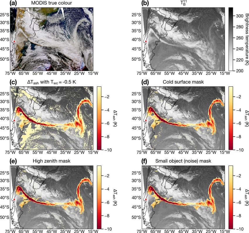
412 A. T. Prata et al.: FALL3D-8.0 – Part 2
Table 3. Description of the files in the Etna-2013 test suite folder (see Sect. 3.3).
Subfolder File Description
InputFiles etna-2013.inp FALL3D-8.0 input file
etna-2013.tgsd.tephra Total grain size distribution (TGSD) file (not generated by the SetTgsd pre-process task)
etna-2013.pts Tracking points file (coordinates of the 10 ground observation locations)
Meteo/ERA5 download_ERA5_sfc_etna2013.py Python script to download ERA5 surface variables in grib2 format1
download_ERA5_ml_etna2013.py Python script to download ERA5 model level variables in grib2 format1
Meteo/WRF namelist.wps Etna-2013 input file for the WRF Pre-Processing System (WPS)
namelist.input Etna-2013 input file for both the real.exe and wrf.exe executables
Validation validate_etna.py Python script to validate model results; writes deposit metrics on validation_etna.csv2
validation_etna_expected.csv Expected results file; should coincide with validation_etna.csv
1 Makes use of CDS API of the Copernicus Climate Data Store. 2 Makes use of pandas, glob, os and sys Python libraries.
olds adopted for the Puyehue case study are provided in Ap- 3.2 Raikoke-2019
pendix A.
On 21 June 2019, a small island volcano, Raikoke
3.1.2 Model setup (48.292◦ N, 153.25◦ E; 551 m a.s.l.), underwent a significant
explosive eruption disrupting major aviation flight routes
To simulate long-range, fine volcanic ash (d ≤ 64 µm) trans- across the North Pacific. Raikoke is located in the central
port from the Puyehue-Cordón Caulle eruption, we carried Kuril Islands, a remote island chain that lies south of Russia’s
out FALL3D runs in two configurations. The first config- Kamchatka Peninsula. Ground-based networks are sparse in
uration (listed as Puyehue-2011 (A) in Table 1) was ini- this area and so satellite observations were crucial for track-
tialised at 21:00 UTC on 4 June 2011 for a duration of 99 h ing the volcanic ash and SO2 produced by the eruption. The
with a continuous emission source term. The source term eruption sequence was characterised by a series of approx-
was defined as a uniform distribution (HAT option) with a imately nine “pulses”, injecting ash and gases into the at-
column height of 11.2 km a.s.l. (9 km above vent level) and mosphere. The International Space Station captured a unique
2 km column thickness. The second configuration (listed as view of the eruption’s umbrella plume during its initial explo-
Puyehue-2011 (B) in Table 1) demonstrates the new data in- sive phase which was reminiscent of the 2009 Sarychev Peak
sertion scheme which was recently introduced in FALL3D- umbrella plume (https://earthobservatory.nasa.gov/images/
8.0 as described in Folch et al. (2020). The data insertion run 145226/raikoke-erupts, last access: 4 November 2020). The
was initialised at 15:00 UTC on 5 June 2011, which coin- eruption sequence was captured extremely well by the
cides with a CALIPSO overpass that intersected the nascent Japanese Meteorological Agency’s Himawari-8 satellite at
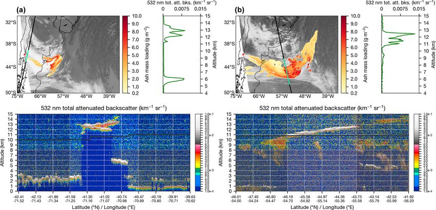
ash plume (see Fig. A4b). To constrain the vertical distribu- both IR and visible wavelengths. According to our analy-
tion of ash in FALL3D, we collocated the CALIOP (Cloud- sis of the satellite data, the initial explosive phase began
Aerosol Lidar with Orthogonal Polarization) total attenuated at around 18:00 UTC on 21 June (05:00 LT1 on 22 June
backscatter profiles with ash-affected SEVIRI pixels. Note at around sunrise) and ended at around 10:00 UTC on 22
that the vertical distribution is only required for the data in- June (21:00 LT just before sunset). The Smithsonian Institu-
sertion time. Based on these coincident observations we set tion’s Global Volcanism Program (GVP) report on the 2019
the cloud-top height and thickness of the data-inserted ash Raikoke eruption also documents less intense activity at the
cloud to 13 km a.s.l. and 2 km, respectively. In addition, to volcano from 23 to 25 June following the initial explosive
account for ash erupted after the data insertion time, we ini- phase (Global Volcanism Program, 2019). During the ini-
tialised the same source term specified in the Puyehue-2011 tial explosive phase on 21 June 2019, a significant amount
(A) configuration (i.e. continuous, uniform source emission of SO2 was injected into the atmosphere making the erup-
up to 11.2 km a.s.l.) at the data insertion time (15:00 UTC on tion an ideal case to study long-range SO2 transport. Pre-
5 June 2011). For both model configurations, the meteoro- liminary analysis of TROPOspheric Monitoring Instrument
logical dataset used was ERA5 reanalysis (Copernicus Cli- (TROPOMI) SO2 retrievals indicated that ∼ 1.4–1.5 Tg SO2
mate Change Service, 2017), which has a horizontal spatial was injected into the atmosphere (Global Volcanism Pro-
resolution of 0.25◦ and 137 model levels. The output do- gram, 2019). Hyman and Pavolonis (2020) present SO2 re-
main size in both cases was set to 15–75◦ S and 20–55◦ W trievals based on Cross-track Infrared Sounder (CrIS) mea-
(0.1◦ latitude–longitude grid resolution). Fine ash species surements and show a time series of SO2 total mass with a
were considered for both model configurations to simulate 1 The local time zone for Raikoke is Magadan Time (MAGT),
airborne PM10 mass loadings. Further details of both model which is UTC+11 and is observed all year. Daylight Savings Time
configurations are summarised in Table 1. (DST) has not been in use in this region since 31 October 2010.
Geosci. Model Dev., 14, 409–436, 2021 https://doi.org/10.5194/gmd-14-409-2021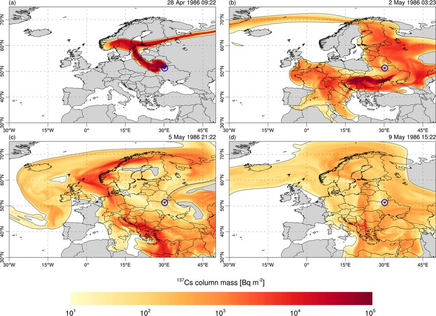
A. T. Prata et al.: FALL3D-8.0 – Part 2                                                                                                   413

Figure 1. Puyehue-2011 test validation results for fine ash mass loading using SEVIRI retrievals on (a) 5 June 2011 at 15:00 UTC (data
insertion time), (b) 6 June 2011 at 15:00 UTC, (c) 7 June 2011 at 15:00 UTC and (d) 8 June 2011 at 15:00 UTC. Left panels show satellite
retrievals with 0.2 g m−2 contour in blue and centre of mass indicated with an “x”. Middle panels show FALL3D fine ash mass loading model
simulation (0.2 g m−2 contour in red). Right panels show spatial overlap of model (shaded in red) vs. observed (shaded in blue) fields with
validation metrics annotated (see Sect. 4 for details). A full animation of the data insertion simulations is available in the Video Supplement
1 (Prata et al., 2020a).

peak between 1 and 1.1 Tg SO2 . These SO2 mass estimates                  2007; Carn et al., 2015; Theys et al., 2017) satellite ob-
suggest that the Raikoke eruption resulted in the largest in-             servations. However, in order to validate FALL3D at high
jection of SO2 into the atmosphere since Nabro (4.5 Tg SO2 )              temporal resolution (hourly or better), geostationary satel-
in 2011 (see Carn et al., 2016, Table 2, for a list of major SO2          lite observations seem preferable. To our knowledge, no
mass injections recorded by satellite).                                   operational geostationary SO2 products are currently avail-
                                                                          able. Therefore, in order to validate the new SO2 scheme in
3.2.1   Validation dataset                                                FALL3D-8.0, we apply the three-channel SO2 retrieval pro-
                                                                          posed by Prata et al. (2003) to the Advanced Himawari Im-
Existing volcanic SO2 datasets are mainly based on polar-                 ager (AHI) instrument aboard the Himawari-8 geostationary
orbiting IR (e.g. Realmuto et al., 1994; Watson et al., 2004;             satellite (Bessho et al., 2016). We selected the AHI due its ex-
Prata and Bernardo, 2007; Corradini et al., 2009; Clarisse                ceptional spatial and temporal coverage during the Raikoke
et al., 2012; Carboni et al., 2016) and UV (e.g. Yang et al.,

https://doi.org/10.5194/gmd-14-409-2021                                                          Geosci. Model Dev., 14, 409–436, 2021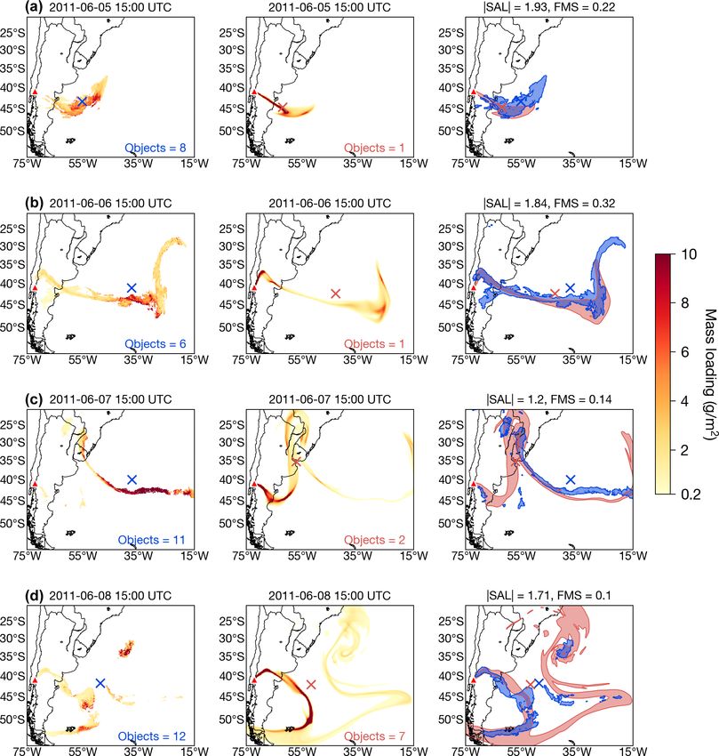
414 A. T. Prata et al.: FALL3D-8.0 – Part 2
eruption. For IR wavelengths, AHI samples the Earth’s full 150–210◦ E (0.1◦ latitude–longitude grid resolution). More
disk every 10 min with a spatial resolution of 2 km × 2 km details of the SO2 model configurations can be found in Ta-
at the subsatellite point. As we did for the SEVIRI ash re- ble 1.
trievals (see Sect. 3.1.1), we resampled the AHI data from
their native resolution to a regular grid (spatial resolution of 3.3 Etna-2013
0.1◦ × 0.1◦ ) and output the retrievals at 1 h temporal reso-
lution for comparison with FALL3D simulations. The ob- On 23 February 2013, the eruptive activity of Mt. Etna in-
servational time period considered for the Raikoke case is creased significantly and at 18:15 UTC a buoyant plume rose
from 18:00 UTC on 21 June 2019 to 18:00 UTC on 25 June up to 9 km a.s.l. (5.68 km above the vent) along with in-
2019 (97 time steps). Details of the implementation of the candescent lava fountains exceeding 500 m above the crater
Prata et al. (2003) retrieval scheme and methods used to de- (Poret et al., 2018). The resulting ash plume extended to-
tect volcanic SO2 for the Raikoke eruption are provided in wards the NE for more than 400 km away from the source,
Appendix B. The retrievals presented here indicate a max- and moderate ash fallout was observed throughout the Ital-
imum total mass of ∼1.4 Tg SO2 , which is in broad agree- ian regions of Calabria and Puglia. Due to the extensive field
ment with other satellite-based SO2 mass estimates (∼ 1– work carried out following the 2013 Mt. Etna eruption, it is
1.5 Tg SO2 ; Global Volcanism Program, 2019; Hyman and an ideal case for validating simulations of tephra ground de-
Pavolonis, 2020). The present SO2 retrieval scheme was orig- posits.
inally developed for HIRS2 (High-resolution Infrared Radia-
3.3.1 Validation dataset
tion Sounder) data. The error budget from Prata et al. (2003)
suggests that errors from 10 % to 20 % are to be expected for To validate tephra deposition from the 2013 Mt. Etna erup-
detectable SO2 column loads up to 800 DU. We expect that tion, we use the ground deposit observations reported by
the Himawari-8 retrieval errors will be of similar magnitude Poret et al. (2018), which consist of measurements of mass
or better. loading per unit area and local grain size distribution (GSD)
obtained by sieve analysis (except for the farthest sample,
3.2.2 Model setup which required a different experimental technique for the
measurement of GSD). Samples were collected a few hours
For volcanic SO2 dispersion from the Raikoke eruption, after the volcanic eruption at 10 different locations (S1–S10).
the test suite considers two simulations to validate the new Locations of sampling sites S7–S10 are indicated in Fig. 6.
SO2 option in FALL3D in the same fashion as the vol- Proximal sites (S1–S7) are located between 5 and 16 km
canic ash simulations (i.e. simulations with and without from the vent, whereas the rest of samples (S8–S10) cor-
data insertion). The model configuration without data in- respond to the locations of Messina (Sicily, S8), Cardinale
sertion (listed as Raikoke-2019 (A) in Table 1) was ini- (Calabria, S9) and Brindisi (Puglia, S10), the latter located
tialised at 18:00 UTC on 21 June 2019, which coincides about 410 km from the volcano.
with the onset of the eruption observed by the Himawari-
8 satellite (Sect. 3.2.1). For the SO2 source term, we use 3.3.2 Model setup
a SUZUKI distribution and a variable column height (be-
tween 3.5 and 15.5 km a.s.l., which corresponds to 3–15 km In order to simulate tephra deposition from the Mt. Etna
above vent level) with a source duration of 14 h and total eruption, we use high-resolution wind fields generated from
runtime of 72 h (Table 1). The data insertion model con- the ARW (Advanced Research WRF) core of the WRF
figuration (listed as Raikoke-2019 (B) in Table 1) was ini- (Weather Research and Forecasting) model (Skamarock
tialised at 18:00 UTC on 22 June 2019 (1 d after the begin- et al., 2008) on a single-domain configuration consisting of
ning of the eruption) as this is a time when the SO2 cloud was 700 × 700 grid points with horizontal resolution of 4 km and
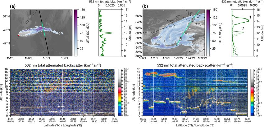
completely detached from source (Fig. 4a). Based on several 100 vertical levels with a maximum height of 50 hPa. The
collocations of CALIOP attenuated backscatter profiles with initial and boundary conditions for the WRF-ARW were ex-
SO2 -affected AHI pixels (e.g. Fig. B3), we set the SO2 cloud- tracted from hourly ERA5 reanalysis data (Copernicus Cli-
top height and thickness to 13.5 and 2.5 km, respectively, at mate Change Service, 2017), which has a spatial resolu-
the data insertion time. We note that CALIOP total attenuated tion of 0.25◦ and 137 vertical model levels. The FALL3D
backscatter measurements are not sensitive to SO2 gas and run was initialised with a start time of 18:00 UTC on 23
so we make the assumption that SO2− 4 aerosols were collo- February and with a uniform source distribution (HAT op-
cated with SO2 in order to assess the likely heights and thick- tion) reaching 5.5 km above the vent (i.e. 8.7 km a.s.l.) and
nesses of the Raikoke SO2 clouds (Carboni et al., 2016; Prata a thickness of 3.5 km. We considered a constant mass flow
et al., 2017). For both model configurations, the meteorolog- rate (3.814 × 10⁵ kg s−1 ) between 18:15 and 19:18 UTC on
ical dataset used was GFS forecast (NCEP, 2015), which has 23 February 2013. The model was configured with a hori-
a horizontal spatial resolution of 0.25◦ and 34 pressure levels. zontal resolution of 0.015◦ and 60 vertical levels up to 11 km
The output domain size in both cases was set to 35–65◦ N and in a computational domain comprising all deposit sampling
Geosci. Model Dev., 14, 409–436, 2021 https://doi.org/10.5194/gmd-14-409-2021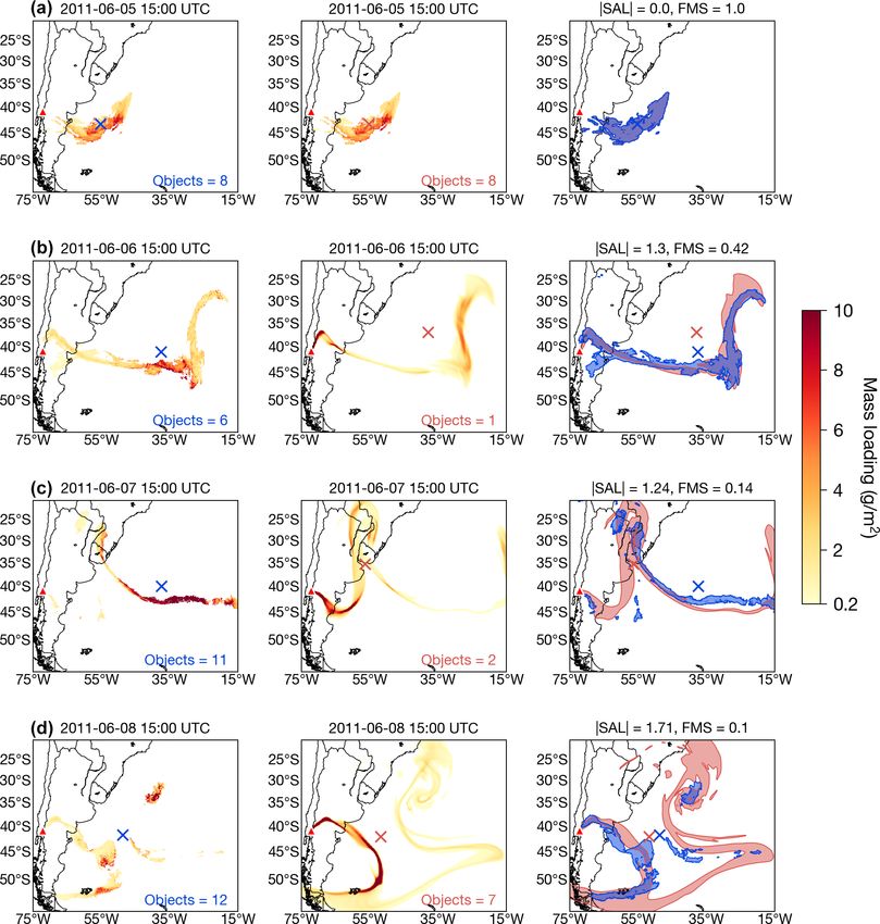
A. T. Prata et al.: FALL3D-8.0 – Part 2                                                                                       415

locations. The particle total grain size distribution (TGSD)     3.4.2    Model setup
was discretised into 32 bins with diameter in 8 units in the
range −68 ≤ d ≤ 68 (diameter can be expressed in mil-            The ability to simulate the transport and deposition of ra-
limetres through the relationship d = 2−8 ), densities varying   dionuclides is a new feature in FALL3D-8.0. In order to sim-
between 1000 and 2500 kg m−3 for coarser and finer bins, re-     ulate the dispersion of radioactive material, estimations of
spectively, and a constant sphericity of 0.92. This test case    the emission rate and of the particle size distributions and
considers a bi-Gaussian (in 8) TGSD defined as                   settling velocities of radioactive material (e.g. 134 Cs, 137 Cs
                                                                 and 131 I isotopes) are needed. Unfortunately, existing estima-
                         (8 − µc )2

            p                             1−p                    tions of such parameters are uncertain due to obvious in situ
f (8) = √ exp −                  2
                                      + √
         σc 2π               2σc         σf 2π                   measurement difficulties and to the interaction of isotopes
                           2
                             !                                   with other atmospheric particles and aerosols (Brandt et al.,
                (8 − µf )
         exp −                 ,                           (1)   2002), and rely on reconstructions and/or on best fitting the
                   2σf2                                          available measurements in the region of interest at the time of
                                                                 the accident. For example, on the basis of high-quality depo-
where µf and σf are the mean and standard deviation for the      sition measurements from the REM database (De Cort et al.,
fine subpopulation, µc and σc are the mean and standard de-      2007), Brandt et al. (2002) reconstructed the source term and
viation for the coarse subpopulation, and p and 1 − p the        identified two emission phases with different vertical mass
relative weight of each subpopulation. Poret et al. (2018)       distributions. The Chernobyl-1986 test suite case uses the
performed numerical simulations using p = 0.59, subpopu-         source term reported by Brandt et al. (2002), parameterised
lation means of µc = −2.96, µf = 0.49, and standard devi-        using the SUZUKI and HAT options in FALL3D (see Ta-
ations of σc = 1.03, σf = 0.79, for coarse and fine popula-      ble 1 for more details of the input parameters). On the other
tions, respectively. However, as already noted by Poret et al.   hand, effective settling velocities typically range from 0.5 to
(2018), such a TGSD underestimates the fine ash fraction.        5 mm s−1 for 137 Cs and from 1 to 20 mm s−1 for 131 I (Brandt
In order to correct this drawback when using a bi-Gaussian       et al., 2002). Considering these ranges and discretising ve-
TGSD, the Etna-2013 test case was run considering a finer        locities into four classes (see Table 5), we chose the effective
TGSD having µc = −2.96, σc = 1.03, µf = 2.54, σf = 0.38,         classes and fractions for Chernobyl-1986 based on the best
and p = 0.7 (note that the latter parameters were calibrated     fit of the simulations with the measured deposit radioactivity
through a trial-and-error procedure). Table 1 summarises         on 10 May 1986. The best fit was performed by changing the
the rest of model configuration options and the final tephra     nuclide size distribution (each class having a different set-
ground load map for a simulation time of 10 h is shown in        tling velocity) and keeping the total mass constant. Minimi-
Fig. 6.                                                          sation was performed through a regular grid search varying
                                                                 the relative weights of the nuclide size classes between 0 and
3.4     Chernobyl-1986
                                                                 1 at steps of 0.01. The Chernobyl-1986 case considers the
One of the most serious nuclear accidents on Earth occurred      computational domain shown in Fig. 8 for the period from
on 25 April 1986 at 21:23 UTC at the Chernobyl nuclear           24 April to 10 May 1986, considering the input values re-
power plant (NPP) in Ukraine. The radioactive material re-       ported in Table 5 and the meteorological fields obtained from
leased as a consequence of two explosions at the NPP was         ERA5 reanalysis, which accounts for atmospheric diffusion,
transported by atmospheric winds thousands of kilometres         wet deposition and radioactive decay.
away from the source, resulting in European-wide disper-
sal of several radionuclide isotopes. The availability of the
Radioactivity Environmental Monitoring (REM) database            4     Validation metrics
(De Cort et al., 2007) along with the simulation results of
Brandt et al. (2002) make the 1986 Chernobyl nuclear ac-         4.1     Structure, amplitude and location
cident a good case study to validate the new radionuclide
scheme in FALL3D-8.0.                                            Both qualitative and quantitative validation approaches have
                                                                 been used to validate previous versions of FALL3D against
3.4.1    Validation dataset                                      satellite observations (e.g. Corradini et al., 2011; Folch et al.,
                                                                 2012). The Puyehue-2011 and Raikoke-2019 test suite cases
To validate FALL3D-8.0 radionuclide simulations of the           use the SAL metric (Wernli et al., 2008) to quantitatively
1986 Chernobyl nuclear accident, the test suite considers        compare satellite retrievals of volcanic ash and SO2 to the
the dataset reported by Brandt et al. (2002), who used high-     corresponding simulations with and without data insertion.
quality deposition measurements from the REM database            The SAL metric was originally developed for validation of
(De Cort et al., 2007). The REM data used for validating the     precipitation forecasts against radar and satellite data (Wernli
Chernobyl-1986 case are provided in the test suite public        et al., 2008). However, Dacre (2011) demonstrated its use
repository.                                                      for validation of air pollution simulations, and Wilkins et al.

https://doi.org/10.5194/gmd-14-409-2021                                               Geosci. Model Dev., 14, 409–436, 2021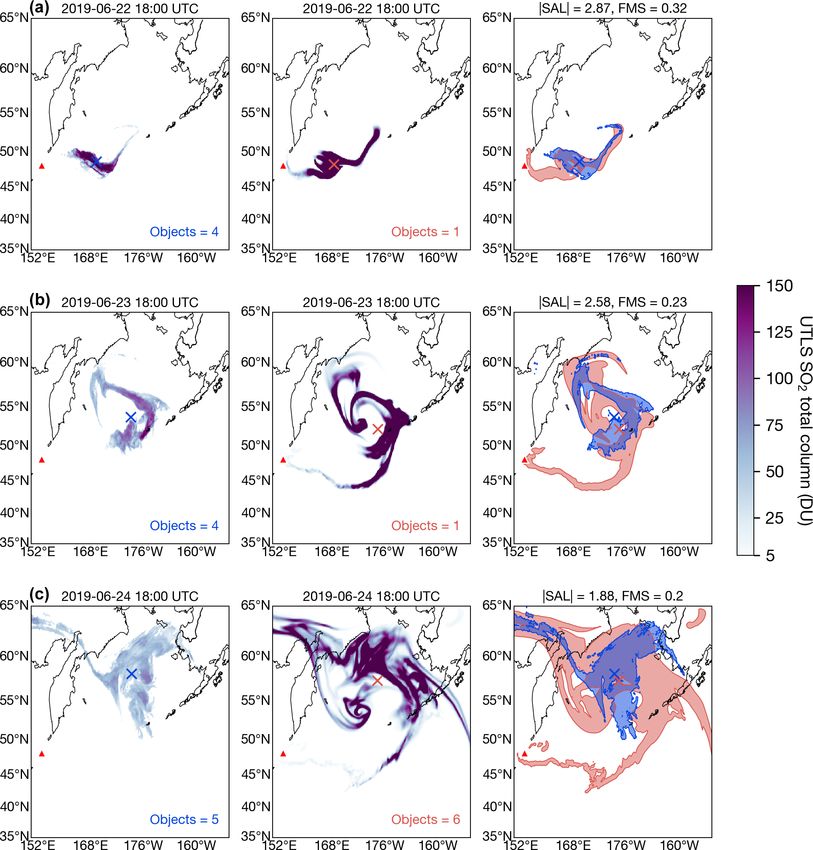
416                                                                                              A. T. Prata et al.: FALL3D-8.0 – Part 2

Table 4. Summary of the SAL and FMS validation scores for the Puyehue-2011 and Raikoke-2019 test suite cases. The “DI” columns
indicate validation scores for runs with data insertion and “NDI” indicates scores for runs with no data insertion.

                 Validation metrics            S              A                     L              |SAL|            FMS
                                          DI         NDI     DI       NDI     DI        NDI       DI    NDI       DI    NDI
                 Puyehue-2011
                 0h                     0.0        −1.31     0.0    −0.5      0.0       0.12      0.0   1.93      1.0   0.22
                 6h                    0.04        −1.48   −0.24   −0.68     0.11       0.08     0.39   2.24     0.56   0.26
                 12 h                 −0.37        −1.68    −0.3   −0.69     0.24       0.05     0.91   2.42     0.48   0.24
                 18 h                 −0.17        −1.57   −0.33   −0.68     0.36       0.07     0.86   2.31     0.43   0.29
                 24 h                  −1.0        −1.22   −0.22   −0.54     0.08       0.09      1.3   1.84     0.42   0.32
                 30 h                  −0.6        −0.85   −0.24   −0.52      0.1       0.12     0.95   1.49     0.38    0.3
                 36 h                 −0.55        −0.77   −0.01   −0.23     0.74       0.75      1.3   1.76      0.4   0.34
                 42 h                  0.46         0.15    0.11   −0.06     0.63       0.37     1.19   0.58      0.3   0.28
                 48 h                 −0.83        −0.84    0.08    0.06     0.32        0.3     1.24    1.2     0.14   0.14
                 54 h                  0.04         0.03    0.41    0.43     0.71       0.67     1.16   1.13     0.11    0.1
                 60 h                  0.64         0.64    0.83    0.83     0.67       0.67     2.15   2.15     0.09   0.09
                 66 h                  0.41         0.41    0.91    0.91     0.45       0.45     1.76   1.76     0.09   0.09
                 72 h                  0.46         0.46    0.89    0.89     0.36       0.36     1.71   1.71      0.1    0.1
                 Raikoke-2019
                 0h                     0.0        −1.18     0.0      1.67    0.0       0.02      0.0   2.87      1.0   0.32
                 6h                   −0.09        −0.98   −0.13      1.63   0.02       0.04     0.24   2.65     0.52   0.28
                 12 h                 −0.24        −1.14   −0.29      1.57   0.04       0.05     0.57   2.76     0.37   0.24
                 18 h                 −0.46        −0.89   −0.46      1.51   0.04       0.04     0.96   2.44     0.31   0.22
                 24 h                 −0.67        −1.03   −0.49       1.5   0.05       0.04     1.21   2.58     0.29   0.23
                 30 h                 −0.62        −0.82   −0.59      1.45   0.05       0.04     1.27   2.31     0.24   0.22
                 36 h                  −0.6        −0.52   −0.58      1.46   0.11       0.09     1.29   2.07     0.25    0.2
                 42 h                 −0.84        −0.52   −0.69       1.4   0.07       0.06      1.6   1.97     0.23   0.21
                 48 h                 −0.68        −0.47   −0.67      1.39   0.03       0.02     1.38   1.88     0.25    0.2

Table 5. Total radioactivity emitted in the atmosphere during the Chernobyl accident in the period 24 April–10 May 1986, for caesium and
iodine isotopes, and their best fit fractions in the considered settling velocity classes.

             Radionuclide     Total activity (PBq)    Vs = 2 mm s−1    Vs = 3 mm s−1           Vs = 4 mm s−1     Vs = 6 mm s−1
             134 Cs                           54               0.54                 0.46
             137 Cs                           85                                                           1.0
             131 I                          1760                                                                               1.0

(2016) employed the SAL for dispersion model validation                magnitude is above some threshold corresponding to a phys-
against IR satellite volcanic ash retrievals for the 2010 Ey-          ical quantity determined from observations. In our case, the
jafjallajökull eruption. More recently, the SAL has also been          threshold is determined based on the detection limit of the
used to compare online vs. offline model simulations of vol-           satellite retrievals. For the SEVIRI ash retrievals (Puyehue-
canic ash (Marti and Folch, 2018). As in Wilkins et al. (2016)         2011 test suite case), we used a threshold of 0.2 g m−2 ,
and Marti and Folch (2018), we also use the FMS score                  consistent with the threshold suggested by Prata and Prata
as a complement to SAL for comparing the spatial cover-                (2012). For the AHI SO2 retrievals (Raikoke-2019 test suite
age of observed vs. modelled fields. A detailed mathematical           case), there is currently no commonly accepted detection
description of the SAL metric is presented in Wernli et al.            threshold. For the purposes of identifying SO2 objects, we
(2008), and so we only provide a brief description of each             allowed for a threshold of 5 DU, noting that the minimum
of the components of SAL (i.e. S, A and L) in the follow-              detected SO2 total column burdens at each time step in the
ing subsections. The main requirement for calculating SAL              satellite retrievals were generally ∼ 8–10 DU. After identify-
is the determination of model and observation “objects”. Ob-           ing objects for both the observation (satellite retrievals) and
jects are identified as clusters of contiguous pixels whose            model fields, we compute the SAL as the sum of the absolute

Geosci. Model Dev., 14, 409–436, 2021                                                          https://doi.org/10.5194/gmd-14-409-2021
A. T. Prata et al.: FALL3D-8.0 – Part 2                                                                                      417

values of S, A and L, which results in an index that varies       vided by the area of union between the ash mass loading ob-
from 0 (best agreement) to 6 (worst agreement). All com-          servation and model fields:
parisons between observations and model simulations were
                                                                            Amod ∩ Aobs
made using a regular 0.1◦ × 0.1◦ latitude–longitude grid.         FMS =                 ,                                    (2)
                                                                            Amod ∪ Aobs
4.1.1    Amplitude                                                where Amod and Aobs are the modelled and observed ash
                                                                  mass loading areas, respectively. The FMS varies from 0 (no
The amplitude (A) metric is the simplest of the three SAL
                                                                  intersection) to 1 (perfect overlap).
components and compares the normalised difference of the
mass-averaged values of the observation and model fields. It      4.3    Root-mean-square error
can vary from −2 to +2, where negative (positive) values
indicate that the model is underpredicting (overpredicting)       The Etna-2013 and Chernobyl-1986 test suite cases use the
the mass when compared with observations.                         RMSE metric to quantitatively compare observations and nu-
                                                                  merical simulations. For this purpose, we consider two vari-
4.1.2    Location                                                 ants of the normalised RMSE, defined as (Poret et al., 2018)
                                                                              v
The location (L) metric has two components (L = L1 + L2 ).                    uN
                                                                              uX
L1 is calculated as the distance between the centres of mass      RMSEj = t        wj (MODi − OBSi )2
between the model and observation objects, normalised by                            i
the maximum distance across the specified domain. It can
                                                                  with
vary from 0 to +1 and is considered a first-order indica-
tion of the accuracy of the model simulation compared with                      1
                                                                  w 1 = PN
observations. However, L1 can equal 0 (suggesting perfect                 OBS2i
                                                                            i
agreement) for situations where observation and model fields           1 1
clearly do not agree. For example, Wernli et al. (2008) de-       w2 =         ,                                             (3)
                                                                       N OBS2i
scribe the case of two objects at opposite sides of the domain
having the same centre of mass as a single object in the centre   where j = 1, 2 depends on the RMSE choice, wj refers to
of the domain. L2 was introduced to handle these situations       the weighting factor used to normalise RMSE, and OBSi and
by considering the weighted average distance between the          MODi are the observed and modelled mass loading related
overall centre of mass and the centre of mass of each individ-    to the ith sample over a set of N samples. The weights cor-
ual object for both model and observation fields. L2 is com-      respond to different assumptions about the error distribution
puted by taking the normalised difference between the model       (e.g. Aitken, 1935; Costa et al., 2009). RMSE1 calculated
weighted average distance and the observation weighted av-        with w1 refers to a constant absolute error, whereas RMSE2 ,
erage distance. It is scaled such that it varies from 0 to +1     calculated using a proportional weighting factor w2 , consid-
(to vary over the same range as L1 ), meaning that L varies in    ers a constant relative error (e.g. Bonasia et al., 2010; Folch
the range from 0 to +2.                                           et al., 2010; Poret et al., 2018).

4.1.3    Structure
                                                                  5     Validation results
The structure (S) metric is the most complex of the three
metrics used to construct SAL. The general idea is to com-        5.1    Puyehue-2011
pute the normalised “volume” of all individual objects for
each dataset (i.e. the model and observation fields). The nor-    Figures 1 and 2 compare satellite retrievals and model simu-
malised volumes are computed by dividing the total (sum)          lations for the Puyehue-2011 case at the data insertion time
mass of each object by its maximum mass. The weighted             (15:00 UTC on 5 June 2011) as well as 24, 48 and 72 h after
mean of the normalised volumes is then computed for the           the insertion time for runs with and without data insertion,
observation and model fields and S is computed by taking          respectively. The time series of each validation metric are
the difference between the weighted means. The S metric           also shown in Fig. 3a, c and summarised in Table 4. Com-
can vary from −2 to +2, where negative values indicate that       parison of Figs. 1a and 2a highlight the advantage of a data
modelled objects are too small or too peaked (or a combina-       insertion scheme to specify model initial conditions. Note
tion of both) compared to the observed fields.                    that for simulations with data insertion at the data insertion
                                                                  time the validation metrics reflect perfect scores (i.e. SAL
4.2     Figure of merit in space                                  of 0 and FMS of 1). For the simulation without data inser-
                                                                  tion (Fig. 2a), the plume has already begun to deviate from
The FMS score compares the spatial coverage of observed           the satellite observations with too much mass dispersing to-
vs. modelled fields. It is simply the area of intersection di-    wards the south. This is reflected in both the SAL score of

https://doi.org/10.5194/gmd-14-409-2021                                                 Geosci. Model Dev., 14, 409–436, 2021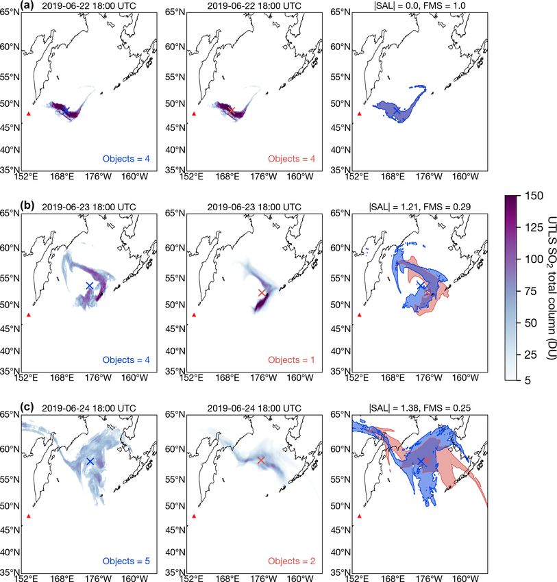
418                                                                                     A. T. Prata et al.: FALL3D-8.0 – Part 2

Figure 2. Same as Fig. 1 but without data insertion.

1.93 and FMS score of 0.22 at this time. The data insertion          Comparison of Figs. 1b and 2b shows that the data inser-
scheme (Fig. 1a) naturally corrects for this by taking advan-        tion simulation is better able to capture the northern portion
tage of good-quality satellite observations of the vertical and      of the plume than the simulation without data insertion at
horizontal structure of the Puyehue ash plume at the insertion       this time (an increase in the FMS by 0.1). Inspection of the
time. For the data insertion simulations, FALL3D accurately          time series of the individual validation metrics for the sim-
represents the spatial structure of the satellite retrievals after   ulations with data insertion (Fig. 3a) reveals that the SAL is
24 h with a SAL score of 1.3 and FMS of 0.42 (Fig. 1b; see           largely being affected by increases in the L metric (i.e. in-
the Video Supplement (Prata et al., 2020a) for the full ani-         creases in the distance between the centres mass between the
mation of the data insertion simulations). In addition, the ac-      observation and model fields) and decreases in the A met-
curacy of the simulations over the first 24 h shows a marked         ric (model underpredicting mass compared to observations).
improvement when compared to the simulations without data            The S metric only exhibits minor deviations when compared
insertion (Fig. 2b; SAL of 1.84; FMS of 0.32). The validation        to the observations during the first 24 h after data insertion.
metric time series show this in more detail (Figs. 3a and b).        At 48 h, the simulations with and without the data insertion
For the simulations without data insertion, the SAL score re-        are almost identical (minor differences in the modelled ash
mains above 2 for most of the first 24 h, while it gradually         contours near 30◦ S, 15◦ W). This is because, at this time,
increases from 0 to 1.3 for the simulation with data insertion.      almost all of the ash used in the data insertion has exited

Geosci. Model Dev., 14, 409–436, 2021                                                  https://doi.org/10.5194/gmd-14-409-2021
A. T. Prata et al.: FALL3D-8.0 – Part 2                                                                                                   419

Figure 3. Time series of validation metrics for (a) Puyehue-2011 test case with data insertion, (b) Raikoke-2019 test case with data insertion,
(c) Puyehue-2011 without data insertion, and (d) Raikoke-2019 without data insertion.

the domain. For the simulations without data insertion, the               5.2   Raikoke-2019
SAL score is 1.2 and FMS is 0.14 (Fig. 2c; Table 4); how-
ever, at around 36 h, SAL reached above 2 and then decreased
                                                                          Figures 4 and 5 show a comparison between the satellite re-
sharply (Fig. 3c). The reason for the sudden reduction in SAL
                                                                          trievals and model simulations with and without data inser-
just after 36 h is most likely due to the satellite retrievals be-
                                                                          tion, respectively, in addition to the SAL and FMS valida-
ing compromised by cloud interference at this time in addi-
                                                                          tion metrics. The time series of validation metrics for the
tion to the continual input of mass due to the emission source
                                                                          Raikoke-2019 case are shown in Fig. 3b and d and are sum-
in the model simulations. Note that this input of mass was
                                                                          marised in Table 4. The AHI retrievals of the SO2 plume at
included to account for ash erupted after the data insertion
                                                                          the beginning of the eruption (Fig. B3a) were likely compro-
time. The satellite retrievals capture some of the ash plume
                                                                          mised by interference of ice particles in the initial eruption
near the source (Figs. 1c and 2c) but cannot be expected to
                                                                          plume (Prata et al., 2003; Doutriaux-Boucher and Dubuis-
accurately characterise the plume at this location due to its
                                                                          son, 2009). In addition, retrievals early on in the plume’s dis-
high opacity in the IR window. Another difference between
                                                                          persion may have been affected by band saturation caused
the model and observations at this time is the large difference
                                                                          by extremely high SO2 column loads. At the data insertion
in the centres of mass (L = 0.32). This is due to the high
                                                                          time (22 June 2019 at 18:00 UTC), the SAL score for the
mass loadings near source in the model fields and high mass
                                                                          SO2 simulation without data insertion is 2.87 and the FMS
loadings near the centre of the domain (43◦ S, 35◦ W) in the
                                                                          is 0.32. Therefore, applying data insertion at this time repre-
observed fields. The satellite is likely overestimating mass in
                                                                          sents a significant correction to the model simulation when
this part of the ash cloud because of underlying water and/or
                                                                          compared against the satellite retrievals (compare Figs. 4a
ice clouds that have not been accounted for in the radiative
                                                                          and 5a). The main difference between the satellite retrievals
transfer modelling. Simulations with and without data inser-
                                                                          and simulation without data insertion is that the model in-
tion are identical after 72 h as all ash used in the data insertion
                                                                          dicates a portion of the SO2 plume connecting back to the
scheme has exited the domain (Figs. 1d and 2d). At this time,
                                                                          volcano, while this feature is not present in the observations.
the SAL reached a score of 1.71 and the FMS has decreased
                                                                          TROPOMI observations of the SO2 cloud confirm this spatial
to 0.10, reflecting a model predictive performance degrading
                                                                          structure (see Fig. 13 of Global Volcanism Program, 2019)
over time.
                                                                          and highlight the importance of understanding the limitations
                                                                          of the AHI retrievals used for data insertion in the present
                                                                          study. The reason for the lack of detection of SO2 in this re-
                                                                          gion in the AHI retrievals is probably due to water vapour in-

https://doi.org/10.5194/gmd-14-409-2021                                                          Geosci. Model Dev., 14, 409–436, 2021
420 A. T. Prata et al.: FALL3D-8.0 – Part 2 Figure 4. Raikoke-2019 validation test results using AHI upper troposphere–lower stratosphere (UTLS) total column burdens retrievals (DU) on (a) 22 June 2019 at 18:00 UTC (data insertion time), (b) 23 June 2019 at 18:00 UTC and (c) 24 June 2019 at 18:00 UTC. Left column shows satellite retrievals with 5 DU contour in blue and centre of mass indicated with an “x”. Middle column shows FALL3D model simulation (5 DU contour in red). Right column shows spatial overlap of model (shaded in red) vs. observed (shaded in blue) fields. A full animation of the data insertion simulations is available in the Video Supplement 2 (Prata et al., 2020b). terference, implying that this part of the plume was at lower imation of the data insertion simulations). Figure 3b shows altitudes than the main SO2 cloud. Indeed, SO2 height re- that the SAL score for the simulation with data insertion is trievals from CrIS data show that plume heights varied from mostly affected by the S and A scores, whereas the L score ∼ 3 to 7 km a.s.l. in this region (see Fig. 5 of Hyman and is low (0.05) indicating that FALL3D is able to track the cen- Pavolonis, 2020). tre of mass of SO2 very well when initialised with satellite For the simulations without data insertion, at 24 h after in- retrievals (Fig. 3b). In this case, the A metric is negative, sertion, the validation metrics exhibit minor changes with meaning that the model is underpredicting the mass when SAL decreasing from 2.87 to 2.59 and the FMS from 0.32 compared to the satellite retrievals. Given that FALL3D-8.0 to 0.23 (Fig. 5a, b). For the simulations with data insertion, does not include SO2 chemistry and only includes SO2 depo- SAL has steadily increased from 0 to 1.21, while the FMS sition mechanisms (Folch et al., 2020), it is unlikely that the has decreased from 1 to 0.29 over the first 24 h (Fig. 4a, b; model is losing SO2 mass too rapidly. Instead, this underpre- see the Video Supplement, Prata et al., 2020b, for the full an- diction is probably being driven by the observed increase in Geosci. Model Dev., 14, 409–436, 2021 https://doi.org/10.5194/gmd-14-409-2021
A. T. Prata et al.: FALL3D-8.0 – Part 2                                                                                        421

Figure 5. Same as Fig. 4 but without data insertion.

mass retrieved by the satellite after the insertion time, which     sublimates in the UTLS (e.g. Rose et al., 2001, 2003, 2004;
cannot be accounted for in the data insertion scheme if no          Guo et al., 2004; Prata et al., 2007; Fisher et al., 2019).
new sources of SO2 are included in the model simulations.              At 48 h, for the simulations without data insertion
An increase in mass, even after the SO2 cloud has detached          (Fig. 5c), the SAL score actually improves (decreasing from
from source, could be related to the detection sensitivity of       2.58 to 1.88) and the FMS largely remains the same (decreas-
the satellite retrieval and the influence of water vapour (Prata    ing from 0.23 to 0.20). The improvement in the SAL score
et al., 2003; Doutriaux-Boucher and Dubuisson, 2009). For           can be attributed to a steady increase in S metric and decrease
example, if the SO2 cloud is in a region of high water vapour       in the A metric (Fig. 3d). This indicates that the structure
initially and then moves into a drier region, it is possible that   and mass (amplitude) simulated without data insertion are
more SO2 will be detected thus increasing the retrieved mass.       converging towards that observed by the satellite over 48 h.
This effect could also occur if the SO2 layers are transported      For the simulations with data insertion, 48 h after insertion
vertically in the atmosphere. Another interesting mechanism         (Fig. 4c), the SAL score continues to increase (from 1.21 to
for the observed increase in SO2 mass after the plume has           1.38) and the FMS continues to decrease (from 0.29 to 0.25).
detached from source is ice–SO2 sequestration. This phe-            In general, at all lead times, the validation metrics indicate
nomenon occurs when ice particles in the nascent plume se-          that the data insertion simulations provide better agreement
quester SO2 initially and then release it later on as the ice

https://doi.org/10.5194/gmd-14-409-2021                                                 Geosci. Model Dev., 14, 409–436, 2021
422                                                                                      A. T. Prata et al.: FALL3D-8.0 – Part 2

Figure 6. Tephra fallout deposit from the Etna-2013 test case. The
spatial distribution of the modelled tephra loading coincides with
the locations of sampling sites. Sites S7–S10 are indicated on the
map by symbols. Proximal sites S1–S6 (< 16 km from the source)
are not shown for clarity.

with observations than the simulations without data insertion
(Table 4).

5.3   Etna-2013

Figure 7a compares modelled and observed tephra loading
for the 2013 Mt. Etna eruption at all observation sites (de-         Figure 7. Comparison between field data at 10 sampling sites (S1–
tailed in Sect. 3.3.1). Note that all points are found within        S10) and results from the Etna-2013 test case. (a) Tephra mass
a factor of 3 around the perfect agreement line (solid black         loading. (b) Mode of the distributions. Field data were obtained
line) across 4 orders of magnitude (from 10−3 kg m−2 to              from the sample dataset reported by Poret et al. (2018).
more than 10 kg m−2 ). This good agreement is also observed
at a bin level in the local grain size distributions. Accord-
ing to the model predictions presented here, unimodal local          (iii) the TGSD used to define the source term; and (iv) the
distributions (negligible ash aggregation effects) are found at      dry deposition parameterisation. Specifically, higher resolu-
all sampling sites, in good agreement with field observations        tion simulations along with the improved numerical scheme
(Poret et al., 2018). In addition, variations of the grain size      implemented in FALL3D-8.0 are expected to lead to a re-
distribution were accurately captured by the simulations as          duction of numerical diffusion errors, which is clearly man-
shown in Fig. 7b, which compares computed and observed               ifested in the spatial distribution of the tephra mass loading
particle distribution modes at all sites (S1–S10).                   field (compare Fig. 6 in the present study to Fig. 6 in Poret
   In terms of the normalised RMSE (see Sect. 4.3), the              et al., 2018). A volcanic ash mass loading simulation for the
model results presented here show a marked improvement               Etna-2013 test suite case is available in the Video Supple-
compared to the FALL3D-7.3 results reported by Poret et al.          ment 3 (Prata et al., 2020c).
(2018). In fact, RMSE1 and RMSE2 reduce from 0.7 and
2.84 in Poret et al. (2018) to 0.58 and 0.98 in this study.          5.4   Chernobyl-1986
The main differences between the simulations performed by
Poret et al. (2018) and this study can be attributed to (i) the      Validation for the 1986 Chernobyl nuclear accident was car-
horizontal resolution of both the meteorological input data          ried out using the normalised RMSE with a constant absolute
and the dispersal model; (ii) the vertical coordinate system;        error (i.e. RMSE1 with w1 ). Since the measured radioactiv-

Geosci. Model Dev., 14, 409–436, 2021                                                  https://doi.org/10.5194/gmd-14-409-2021
A. T. Prata et al.: FALL3D-8.0 – Part 2                                                                                                423

Figure 8. Chernobyl-1986 accumulated total deposition of 137 Cs
on 10 May 1986. The underlying map is reported just for reference   Figure 9. Comparison between measurements and Chernobyl-
and could contain nations’ borders that are under dispute.          1986 test deposit results of 137 Cs, 134 Cs and 131 I at different loca-
                                                                    tions on 10 May 1986. The solid line represents one-to-one agree-
                                                                    ment between measured and modelled values. Lower and upper
ity spans over 4 orders of magnitude, the RMSE1 was calcu-          dashed lines represent factors of 0.1 and 10, respectively, from the
lated between the logarithms of the measured and modelled           one-to-one line.
radioactivity values at different tracking points (29 for 131 I,
44 for 134 Cs and 45 for 137 Cs, from the REM database). The
obtained values of RMSE1 are 0.10, 0.09 and 0.06 for 131 I,
134 Cs and 137 Cs, respectively. A map showing the 137 Cs de-
                                                                    ash dispersal and SO2 cloud dispersal, respectively. The met-
posit distribution simulated can be found in Fig. 8. The com-       rics used for validation were the SAL and FMS and were
parison of measured and simulated values for the best fit-          applied to simulations with and without data insertion. To
ted terminal velocity bins (Table 5) is shown in Fig. 9. Note       characterise the vertical structure of these volcanic clouds
that most of simulated values lie within an order of mag-           at selected data insertion times, geostationary satellite ob-
nitude of the measurements (Fig. 9). Simulation results of          servations were collocated with CALIPSO overpasses. Ac-
the radioactive cloud evolution relative to 137 Cs (vertically      cording to the SAL and FMS metrics, simulations initialised
integrated radioactivity concentration in the atmosphere, ex-       with data insertion consistently outperform simulations with-
pressed in Bq m−2 ) from 28 April to 9 May 1986, are shown          out data insertion. For the data insertion simulations, SAL
in Fig. 10. Figure 10 shows that the Chernobyl-1986 simu-           remained below 1 out to 18 h (Table 4) and below 2 at lead
lations correctly reproduce the patterns described by Brandt        times of 24 and 48 h for both ash and SO2 simulations. While
et al. (2002). The evolution of the 137 Cs dispersal is also        it is not yet clear what absolute values of SAL and FMS
available as a video in the Video Supplement 5 (Prata et al.,       should represent an acceptable ash/SO2 forecast, it is un-
2020e), together with videos corresponding to the dispersal         likely that in an operational setting a model simulation would
of 134 Cs (Video Supplement 4; Prata et al., 2020d) and 131 I       be relied upon beyond 48 h. Ideally, the model should be re-
(Video Supplement 6; Prata et al., 2020f).                          run with an updated data insertion time when new, good-
                                                                    quality satellite retrievals become available. Based on our
                                                                    findings, it appears that SAL values of less than 1.5 and FMS
6   Conclusions                                                     values greater than 0.40 indicate good spatial agreement be-
                                                                    tween the model and observation fields (e.g. Fig. 1b). How-
Four different examples from the new FALL3D-8.0 bench-              ever, it is important to consider that the satellite retrievals can
mark suite have been presented to validate the accuracy of          be affected by several factors (e.g. cloud interference, high
the latest major version release of the FALL3D model and            water vapour burdens, chosen detection thresholds) meaning
complement a companion paper (Folch et al., 2020) on model          that the ash/SO2 detection schemes may miss some legiti-
physics and performance. In the first two examples, geosta-         mate ash or SO2 that the model is otherwise predicting (e.g.
tionary satellite observations from Meteosat-9 (SEVIRI) for         Fig. 1c). Limitations of the observations should also be taken
the 2011 Puyehue-Cordón Caulle eruption (i.e. Puyehue-              into account when initialising simulations with data inser-
2011 test suite case) and from Himawari-8 (AHI) for the             tion. A data assimilation scheme that considers the errors in
2019 Raikoke eruption (i.e. Raikoke-2019 test suite case)           the satellite retrievals in addition to errors in the model sim-
were used to validate FALL3D simulations of far-range fine          ulations (e.g. using an ensemble approach to generate proba-

https://doi.org/10.5194/gmd-14-409-2021                                                    Geosci. Model Dev., 14, 409–436, 2021
You can also read