The first Met Office Unified Model/JULES Regional Atmosphere and Land configuration, RAL1
←
→
Page content transcription
If your browser does not render page correctly, please read the page content below
The first Met Office Unified Model/JULES Regional Atmosphere
     and Land configuration, RAL1
     Mike Bush1 , Tom Allen1 , Caroline Bain1 , Ian Boutle1 , John Edwards1 , Anke Finnenkoetter1 ,
     Charmaine Franklin2 , Kirsty Hanley1 , Humphrey Lean1 , Adrian Lock1 , James Manners1 ,
     Marion Mittermaier1 , Cyril Morcrette1 , Rachel North1 , Jon Petch1 , Chris Short1 , Simon Vosper1 ,
     David Walters1 , Stuart Webster1 , Mark Weeks1 , Jonathan Wilkinson1 , Nigel Wood1 , and
     Mohamed Zerroukat1
     1
         Met Office, FitzRoy Road, Exeter, EX1 3PB, UK
     2
         Bureau of Meteorology (BoM), Melbourne, Victoria, Australia
     Correspondence: Mike Bush (mike.bush@metoffice.gov.uk)

     Abstract. In this paper we define the first "Regional Atmosphere and Land" (RAL) science configuration for kilometre scale
     modelling using the UM and JULES. "RAL1" defines the science configuration of the dynamics and physics schemes of the
     atmosphere and land. This configuration will provide a model baseline for any future weather or climate model developments
     to be described against and it is the intention that from this point forward significant changes to the system will be documented
5    in literature. This is reproducing the process used for global configurations of the UM which was first documented as a science
     configuration in 2011. While it is our goal to have a single defined configuration of the model that performs effectively in all
     regions, this has not yet been possible. Currently we define two sub-releases, one for mid-latitudes (RAL1-M) and one for
     tropical regions (RAL1-T). The differences between RAL1-M and RAL1-T are documented and where appropriate, we define
     how the model configuration relates to the corresponding configuration of the global forecasting model.

10   Copyright statement. This work is distributed under the Creative Commons Attribution 3.0 License together with an author copyright. This
     license does not conflict with the regulations of the Crown Copyright.

     1     Introduction

     It is becoming standard practice for National Met Services (NMS) and those involved in the prediction of high-impact weather
     to use regional atmospheric and land models with grid-lengths of the order of a kilometre as their prediction systems (e.g. Klasa
15   et al. (2018)). While not truly resolving deep convection, kilometre scale atmospheric models are able to explicitly represent
     deep convective processes within the resolved dynamics. These models provide valuable information on local weather and
     high-impact weather that is critical to the core function of NMSs. The representation of convective systems, topographically
     driven weather and various mesoscale features are generally improved with these regional modelling systems (Clark et al.,
     2016). In addition to weather forecasting, kilometre scale simulations are now emerging as a tool for climate projections (e.g.

                                                                          1
Kendon et al. (2017)). While there is significant computational cost to running regional models with grid-length of order
     kilometre scale for the many long duration runs needed for climate projections, the value of the far improved representation of
     weather systems, especially those related to high-impact weather, makes the computational costs worthwhile.
       The Met Office’s primary operational deterministic numerical weather prediction (NWP) weather forecast system over the
5    United Kingdom (the UKV, Tang et al. (2013)) and ensemble prediction system (MOGREPS-UK, Hagelin et al. (2017)) are run
     with grid-lengths of order of a kilometre. These systems both use the Met Office Unified Model (UM, Brown et al. (2012)) as
     the basis for the atmosphere and the Joint UK Land Environment Simulator (JULES, (Best et al., 2011; Clark et al., 2011)) for
     the land. They are run in variable resolution mode, with horizontal grid-lengths in the central regions of their domains of 1.5km
     and 2.2km respectively. In addition, the Met Office also carry out regional kilometre scale simulations for climate projection,
10   the latest of which have been run with horizontal grid-lengths of 1.5km over a domain covering the Southern UK (Kendon
     et al. (2014)), 2.2km over Europe (Berthou et al. (2018)) and 4.4km over Africa (Stratton et al. (2018)). The exact choice of
     grid-length and domain size is a pragmatic one where the aim is to have as good a resolution as possible while allowing the
     forecasts or climate projections to run in the allotted time on the computer systems available.
       Regional modelling in the Met Office is not confined to the UK for weather or climate. For several international collabo-
15   rations, and to meet various commitments, the Met Office also runs kilometre scale UM simulations in many other regions
     around the world. In addition, as part of the UM partnership, a range of institutions beyond the Met Office also run the regional
     model in their areas of interest. With the many regions and many users of the model it has become more important than ever
     to coordinate its development and have clearly defined science configurations. In this paper we define the first "Regional At-
     mosphere and Land" (RAL) science configuration for kilometre scale modelling using the UM and JULES. "RAL1" defines
20   the science configuration of the dynamics and physics schemes of the atmosphere and land. This configuration will provide
     a model baseline for any future weather or climate model developments to be described against. It is the intention that from
     this point forward significant changes to the system will be documented in literature. This is reproducing the process used for
     global configurations of the UM which was first documented as a science configuration in 2011 (Walters et al. (2011)).
       While it is our goal to have a single defined configuration of the model that performs effectively in all regions, this has not yet
25   been possible. Currently we define two sub-releases, one for mid-latitudes (RAL1-M) and one for tropical regions (RAL1-T).
     The differences between RAL1-M and RAL1-T are clearly documented within this paper. Also, where appropriate, we define
     how the model configuration relates to the corresponding configuration of the global forecasting model defined in Walters et al.
     (2017).
       Prior to the existence of RAL1, there was no single definition for the configuration of the regional UM model. As RAL1 is the
30   first formally documented model configuration there is no previous baseline against which to document performance and recent
     developments. However, it is a goal of this paper to highlight the most recent updates and describe how these have improved
     performance over previous versions of the regional UM system. To do this we focus on the UK and describe the model changes
     against the previous operational weather prediction system. This baseline, known in the Met Office as Operational Suite 37
     (OS37) was the operational system from 15th March 2016 to 08th November 2016 and will be referred to in this paper as
35   RAL0.

                                                                      2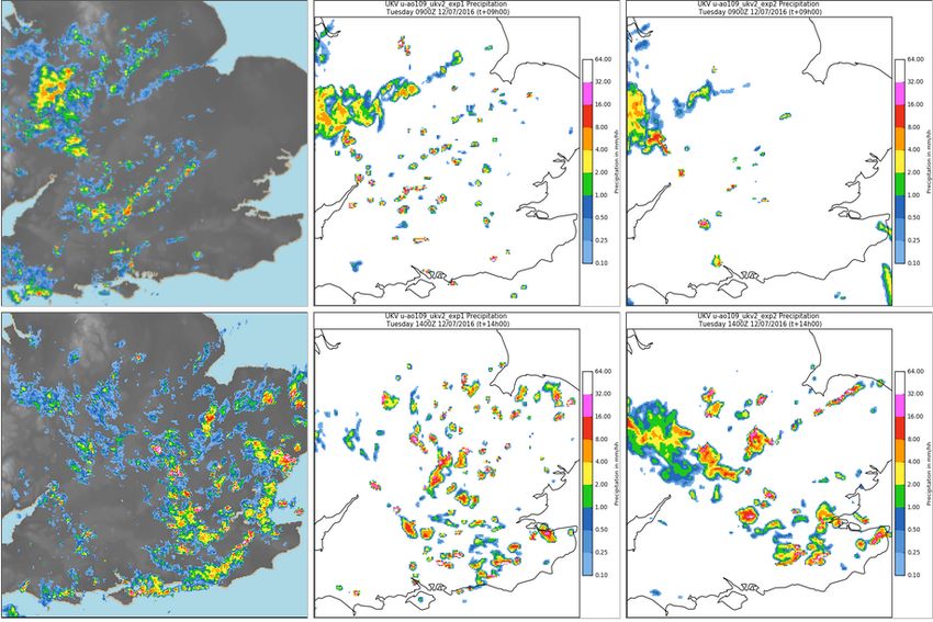
In Sect. 2, we document the RAL0 configuration. In Sect. 3, we highlight the RAL1-M developments which when added
     to the RAL0 base define RAL1-M. In Sect. 4 we document the Tropical version RAL1-T and in Sect. 5 we evaluate the
     performance of RAL1-M and RAL1-T configurations in five parts of the world with different meteorology. Finally, in Sect. 6
     we provide some concluding remarks.

5    2     Defining Regional Atmosphere and Land - version 0 (RAL0)

     2.1    Dynamical core: Spatial aspects

     The primary atmospheric prognostics are the three-dimensional wind components, virtual dry potential temperature, Exner
     pressure, dry density, five moist prognostics (mixing ratios of water vapour, liquid, ice, rain and graupel) and murk aerosol
     (operational UK forecasts only). These prognostic fields are discretised horizontally onto a rotated longitude/latitude grid with
10   the pole rotated so that the grid’s equator runs through the centre of the model domain. Optionally, the horizontal grid may be
     specified as being of variable resolution, where the grid size varies smoothly from coarser resolution at the outer boundaries to
     a uniform fine resolution in the interior of the domain as described in Tang et al. (2013). The prognostic variables are stored
     using Arakawa C-grid staggering (Arakawa and Lamb, 1977) in the horizontal and Charney-Phillips staggering (Charney and
     Phillips, 1953) in the vertical. A terrain-following hybrid height coordinate is used.
15       In the vertical, RAL0 uses a 70 level vertical level set labelled L70(61t , 9s )40 , which has 61 levels below 18 km, 9 levels
     above this and a fixed model lid 40 km above sea level. This naming convention was originally devised for global model
     simulations to denote the maximum number of levels that could be in the troposphere at its maximum depth of around 18 km
     (t ) and the number above this that would always be in the stratosphere or above (s ). As the mid-latitude tropopause is typically
     at a height of roughly 9-11 km, this level set concentrates its levels below 9 km with only 20 of its 70 levels above this. A more
20   detailed description of these level sets is included in the supplementary material to this paper.

     2.2    Dynamical core: Spatio-temporal discretisation

     The UM’s ENDGame dynamical core uses a semi-implicit (SI) semi-Lagrangian (SL) formulation to solve the non-hydrostatic,
     fully-compressible deep-atmosphere equations of motion (Wood et al., 2014). The discrete equations are solved using a nested
     iterative structure for each atmospheric time step within which some terms are lagged and computed in an outer loop, while
25   others are treated quasi-fully implicitly in an inner loop.
         The SL departure point equations are solved within the outer loop using a centred average of the previous time step (time level
     n) wind and the latest estimates for the current time step (time level (n+1)) wind. Appropriate fields are then interpolated to the
     departure points, using Lagrange interpolation, with various polynomial degree options. Since pointwise Lagrange interpolation
     is not a conservative operation, the mass of dry air, the various water species, and any other transported tracers can drift due
30   to numerical errors as well as the net fluxes through the lateral boundaries. The lack of enforcement of the correct budget of

                                                                      3
such fields in RAL0 is the motivation for a change in RAL1 to use of the Zero Lateral Flux (ZLF) scheme of Zerroukat and
     Shipway (2017) which is outlined in section 3.1.
       Within the inner loop, a linear Helmholtz problem is solved to obtain the pressure increment in which the Coriolis, orographic
     and non-linear terms are evaluated as source terms to this equation: they are averaged in an off-centred semi-implicit fashion
5    along the semi-Lagrangian trajectory using both the known state at time level n and the latest estimated (iterated) values of the
     fields at time level (n+1). Having solved the Helmholtz problem, the other prognostic variables are obtained from the pressure
     increment via a back-substitution process (see Wood et al. (2014) for further details). An off-centring of 0.55 is used for all
     variables (where a value of 0.5 represents a centred scheme and a value of 1.0 would be a fully implicit scheme).
       Imposing the lateral boundary conditions (LBCs) within the solution procedure requires special treatment and details of this
10   are given in section 8.
       The physical parametrisations are split into slow processes (radiation and microphysics) and fast processes (atmospheric
     boundary layer turbulence, cloud and surface coupling). The slow processes are treated in parallel and computed using only
     the previous time level n model’s state. They are computed once per time step before the outer loop. The source terms from
     the slow processes are then added explicitly to the appropriate fields before the semi-Lagrangian advection (i.e interpolation).
15   The fast processes are treated sequentially and are computed in the outer loop using the latest estimate for the model state at
     the current time step, or time level (n + 1) (i.e., fast process are treated approximately fully-implicitly as the final state (n + 1)
     cannot be known until the end of the iteration process). A summary of the atmospheric time step is given in Algorithm 1 in
     section 8. In practice two iterations are used for each of the outer and inner loops so that the Helmholtz problem is solved four
     times per time step. Finally, Table 1 contains the typical length of time step used for a range of horizontal resolutions.
20     There are a number of differences between the Limited Area Model (LAM) formulation of ENDGame and the global version
     described in Wood et al. (2014). An important one of these arises due to the iterative nature of the ENDGame algorithm and
     the requirement, in practice, to apply LBCs over the area covered by Ω2 and Ω3 in Figure 1. Algorithm 1 gives an outline of a
     typical ENDGame time step with the primary difference being the addition of the expected updating of the LAM LBCs at the
     end of each time step but also the addition of an update dynamics only LBCs step during the main iteration. The main purpose
     of this step is to reset the new time level’s velocities to be compatible with the LBCs since these will have been altered in the
     Helmholtz/inner loop section.

     Table 1. Typical time step for a range of horizontal resolutions.

                                        Radial resolution    Nominal physical resolution   Typical time step

                                        0.0135◦                          1.5 km                         60 s
                                             ◦
                                        0.02                             2.2 km                       100 s
                                             ◦
                                        0.04                             4.4 km                       100 s

                                                                           4
2.3    Lateral Boundary Conditions (LBCs)

     LAMs solve the atmospheric equations on a physical domain Ω1 subject to LBCs provided by a driving (generally a global)
5    model, imposed on the periphery of Ω1 (see Figure 1). The UM’s treatment of LBCs uses the method of relaxation/blending
     (Davies, 1976; Perkey and Kreitzberg, 1976). The relaxation method requires the LBCs to be a data region (shown in Figure 1
     by the RIM region Ω2 + Ω3 ) with several grid points so that the driving model (or LBCs) and the LAM solutions are gradually
     blended to reduce wave reflections from the boundaries (Marbaix et al., 2003). Additionally, for SL models the LBCs are
     further extended, as a fluid parcel ending up inside the domain Ω1 may have come from a region outside Ω1 and far away from
10   its boundary Γ1 depending on the scale of the horizontal wind and the size of the time step used. The number of points defines
     the size of the LBCs and depends on the order of interpolation used for SL advection, the size of the blending zone and the
     maximum (expected) Courant number allowed (Aranami et al., 2014). The UKV model uses Ω2 = 3, Ω3 = 5 and Ω4 = 7.
       The solver is identical in structure between LAM and global with the application of the boundary conditions on the
     Helmholtz equation being the main difference. The pressure boundary condition is of Dirichlet type with the (hydrostati-
15   cally balanced) LBC held fixed on the outer most part of Ω3 . LBC vertical velocity is assumed to be zero while that obtained
     from the inner loop will be non-zero. An implicit vertical damping profile is employed whose damping rate is proportional to
     the blending weights used in regions Ω2 and Ω3 . Not only does this help with the model imbalance it also reduces the iteration
     count of the linear solver while also improving model stability.
       Another difference between the LAM models and global is the calculation of trajectories (departure points) for the SL
20   transport. The absence of the polar singularity allows for a much simpler (less computationally expensive) departure point
     algorithm, compared to Thuburn and White (2013), and is essentially described in Allen and Zerroukat (2016) but with the
     additional constraint of the departure points being clipped to Ω3 in Figure 1. At excessively large Courant numbers, which can
     occur sporadically when the jet stream intersects the lid of the model, there is the potential for the data required to interpolate the
     fields to be off-processor. The solution is derived from observing that for a halo width H and for cubic Lagrange interpolation,
25   the largest westward Courant number allowable is H − 1 while the largest eastward Courant number is H − 2 and similarly for
     North and South. This observation allows for the introduction of a trajectory clipping algorithm which looks at the distance
     of the departure point (in grid point space) from the arrival point and moves it, depending on the direction of the flow, if the
     distance is greater than the maximum allowable to the furthest grid point at which there would be no issues. At points that
     have been moved the interpolation weights are reset to 0.5 to remove any potential biases. Note that, because this calculation is
30   performed in grid point space, the variation of the Courant number with the variable grid resolution is automatically accounted
     for.

     2.4    Solar and terrestrial radiation

     Shortwave (SW) radiation from the Sun is absorbed and reflected in the atmosphere and at the Earth’s surface and provides
     energy to drive the atmospheric circulation. Longwave (LW) radiation is emitted from the planet and interacts with the at-
     mosphere, redistributing heat, before being emitted into space. These processes are parametrised via the radiation scheme,

                                                                       5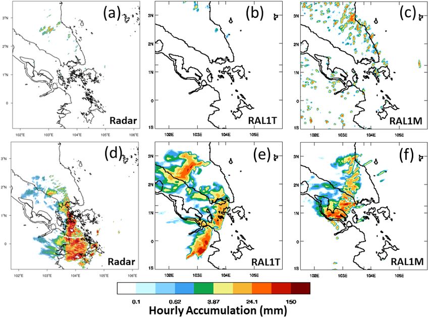
which provides prognostic atmospheric temperature increments, prognostic surface fluxes and additional diagnostic fluxes.
                          1
     The SOCRATES             radiative transfer scheme (Edwards and Slingo, 1996; Manners et al., 2018) is used with a configuration
5    based on GA3.1 (Walters et al., 2011). Solar radiation is treated in 6 SW bands and thermal radiation in 9 LW bands. In the
     LW an approximate treatment of scattering is used (Manners et al., 2018) to reduce execution time.
       Gaseous absorption uses the correlated-k method with coefficients identical to the GA3.1 configuration. Twenty-one (21) k terms
     are used for the major gases in the SW bands, with absorption by water vapour (H2 O), carbon dioxide (CO2 ), ozone (O3 ), and
     oxygen (O2 ). Thirty-three (33) k terms are used for the major gases in the LW bands, with absorption by H2 O, O3 , CO2 , CH4 ,
10   N2 O, CFC-11 (CCl3 F) and CFC-12 (CCl2 F2 ). Of the major gases considered, only H2 O is prognostic; O3 uses a climatology,
     whilst other gases are prescribed using a fixed mass mixing ratios and assumed to be well mixed.
       Absorption and scattering by aerosols is included based on a simple climatology of five species: water soluble, dust, oceanic,
     soot and stratospheric aerosols. The component in the planetary boundary layer is distributed over approximately 3.2km of the
     atmosphere (lowest 30 model levels) and the contribution from dust has been scaled by 0.3333 compared to the original
15   climatology of Cusack et al. (1998).
       The parametrisation of cloud droplets is described in Edwards and Slingo (1996) using the method of “thick averaging”.
     Padé fits are used for the variation with effective radius, which is computed from the number of cloud droplets calculated in
     the microphysics scheme (see section 2.5). The parametrisation of ice crystals is described in Baran et al. (2016).
       The sub-grid cloud structure is represented using separate cloud fractions for the liquid and ice components with the liquid
20   water mass mixing ratio scaled by a factor of 0.7 to represent the effect of cloud inhomogeneity as described in Cahalan et al.
     (1994). Cloud fractions in adjacent layers in the vertical are maximally overlapped, while clouds separated by clear-sky are
     randomly overlapped. Full radiation calculations are made every 15 min using the instantaneous cloud fields and a mean solar
     zenith angle for the following 15 min period. Corrections for the change in solar zenith angle on every model time step and the
     change in cloud fields every 5 min are made as described in Manners et al. (2009).
25     The emissivity and the albedo of the surface are set by the land surface model. The direct SW flux at the surface is corrected
     for the angle and aspect of the topographic slope and for shading by surrounding terrain. The net LW flux at the surface is
     corrected for the resolved sky-view factor due to the surrounding terrain (Manners et al., 2012).

     2.5   Microphysics

     The formation and evolution of precipitation due to grid scale processes is the responsibility of the microphysics scheme. The
30   microphysics scheme has prognostic input fields of temperature, moisture, cloud and precipitation from the end of the previous
     time step, which it modifies in turn. The microphysics used is a single moment scheme based on Wilson and Ballard (1999),
     with extensive modifications. We make use of prognostic rain, which allows three-dimensional advection of the rain mass
     mixing ratio. This has been shown to improve precipitation distributions over and around mountainous regions, especially with
     the smaller grid spacings used in the RAL configurations (Lean et al., 2008; Lean and Browning, 2013). Prognostic graupel
     has also been included, this allows for the explicit representation of a second, more dense ice category which is useful for hail
       1 https://code.metoffice.gov.uk/trac/socrates

                                                                       6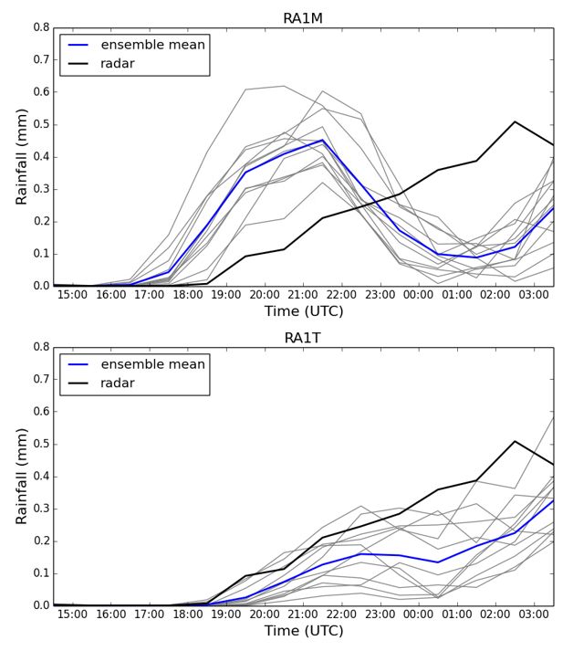
forecasting at kilometre scale resolutions as well as being a prerequisite for lightning forecasting (Wilkinson and Bornemann,
     2014).
5      The warm-rain scheme is based on Boutle et al. (2014b), and includes an explicit representation of the affect of sub-grid
     variability on autoconversion and accretion rates (Boutle et al., 2014a). We use the rain-rate dependent particle size distribution
     of Abel and Boutle (2012) and fall velocities of Abel and Shipway (2007), which combine to allow a better representation of
     the sedimentation and evaporation of small droplets. The cloud droplet number concentration can be determined from assuming
     either a) a fixed climatological aerosol, or b) using a single-species prognostic aerosol which has been developed for forecasts
10   of visibility (Clark et al., 2008). For the cases where single-species prognostic aerosol is used, the aerosol concentrations are
     coupled to the cloud drop number using the methodology described in Wilkinson et al. (2013) and modified following Osborne
     et al. (2014). In the case of the fixed climatological aerosol, the parametrisation of Jones et al. (1994) is used. In both cases,
     droplet numbers are reduced near the surface for effective fog simulation and changes included in RAL1 are described in
     section 3.3).
15     Ice cloud parametrisations use the generic size distribution of Field et al. (2007) and mass-diameter relations of Cotton et al.
     (2013). The fall speed of ice used is the dual fall-speed as described in Furtado et al. (2015), where the lowest value of two
     computed fall speed relations is used; this represents the fact that the Field et al. (2007) parametrisation includes contributions
     from both smaller ice crystals and larger ice aggregates.
       Unlike the GA configurations, there is no requirement for multiple sub-time stepping of the microphysics scheme as the
20   model time step in the RAL configurations is shorter than the 2-minute period used as a sub-time step in the GA configurations.
       As in Stratton et al. (2018), the output taken immediately after the microphysics scheme drives a lightning parametrisation,
     based on McCaul et al. (2009); with the discharge of lightning flashes in the column being determined as described in Appendix
     A of Wilkinson (2017). This has been shown to be of benefit for a high-profile event (Wilkinson and Bornemann, 2014) and to
     perform well during the summer months (Wilkinson, 2017).

25   2.6   Large-scale cloud

     Due to sub-grid inhomogeneity, clouds will form well before the humidity averaged over the size of a grid-box reaches satura-
     tion and this is still true when grid-box size is at the kilometer scale (Boutle et al., 2016). A cloud parametrisation scheme is
     therefore required to determine the fraction of the grid-box which is covered by cloud and the amount and phase of condensed
     water contained in those clouds. The formation of clouds will convert water vapour to liquid or ice and release latent heat. The
30   cloud cover and liquid and ice water contents are then used by the radiation scheme to calculate the radiative impact of the
     clouds and by the microphysics scheme to calculate whether any precipitation has formed.
       RAL0 uses the Smith (1990) cloud scheme. This is a diagnostic scheme, in which the cloud cover is calculated only from
     information available at that moment in time. The scheme relies on a definition of critical relative humidity, RHcrit, which
     is the grid-box mean relative humidity at which clouds start to appear. The value of RHcrit is set to 0.96 at the surface and
     decreases monotonically to 0.80 at 850m (model level 15). It is then held fixed above that.

                                                                     7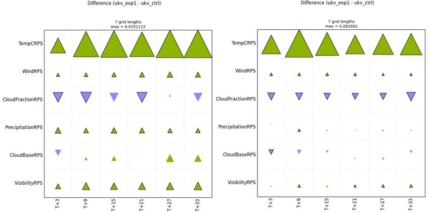
For liquid cloud, the Smith cloud scheme is built around an assumption that sub-grid temperature and humidity fluctuations
     can be described by a symmetric triangular probability distribution function (PDF). One consequence of this PDF assumption
     is that the grid-box has 50% cloud cover when the total relative humidity, RHt=(qv+qcl)/qsat, reaches 100% and that the grid-
5    box only becomes overcast when RHt>=2-RHc. However, observations such as Wood and Field (2000) suggest that the cloud
     fraction should be larger than 0.5 when RHt=100%. As a result, an empirically-adjusted cloud fraction (EACF) is used with
     the Smith scheme in kilometre-scale models. The relative humidity at which cloud first appears is unchanged, but the smooth
     function linking cloud fraction to relative humidity increases more rapidly so that cloud fraction is 0.70 when RHt=100%.
       Forecasts using the EACF still under-estimate cloudiness however, especially the thin clouds forming below a temperature
10   inversion that do not fill the entire depth of a model layer. So an area cloud fraction scheme is also used, which follows a similar
     approach to that described by Boutle and Morcrette (2010). Each model level is split into three and vertical interpolation is
     used to find the thermodynamic values in the sub-layers. However, if there is a strong gradient in RH, due to the presence of
     a capping inversion, the thermodynamic properties of the sub-layer are found by extrapolation from above and below instead.
     This sharpens the inversion and can increase the RH in the sub-layers below it. The Smith cloud scheme, itself modified to use
15   the EACF, is then called on each of the 3 sub-layers. The cloud fraction for use by the microphysics is set to the mean of the
     cloud fractions over the 3 sub-layers, while the cloud fraction seen by radiation is set the maximum of the values from the 3
     sublayers.
       The ice cloud fraction is parametrised as described by Abel et al. (2017) where it is diagnosed from the ice water content.

     2.7   Atmospheric boundary layer

20   The parametrisation of turbulent motions in kilometre scale models requires special treatment because, although most turbulent
     motions are still unresolved, the largest scales can be of a similar size to the grid-length. The model must therefore be able
     to parametrize the smaller scales, resolve the largest ones if possible, and not alias turbulent motions smaller than the grid-
     scale onto the grid-scale. The “blended” boundary-layer parametrisation described by Boutle et al. (2014b) is used to achieve
     this. This scheme transitions from the 1D vertical turbulent mixing scheme of Lock et al. (2000), suitable for low-resolution
25   simulations such as GA configurations, to a 3D turbulent mixing scheme based on Smagorinsky (1963) and suitable for high-
     resolution simulations, based on the ratio of the grid-length to a turbulent length scale. The blended eddy diffusivity, including
     any non-local contribution from the Lock et al. (2000) scheme, is applied to down-gradient mixing in all three dimensions,
     whilst appropriately weighted non-local fluxes of heat and momentum are retained in the vertical for unstable boundary-
     layers. The configuration of the Lock et al. (2000) scheme is similar to that of GA7 (Walters et al., 2017), with differences as
30   follows: (i) for stable boundary layers, the “sharp” function is used everywhere, but with a parametrisation of sub-grid drainage
     flows dependent on the sub-grid orography (Lock, 2012), (ii) heating generated by frictional dissipation of turbulence is not
     represented, and (iii) the parametrisation of shear generated turbulence extending into cumulus layers (Bodas-Salcedo et al.,
     2012) is not used.

                                                                      8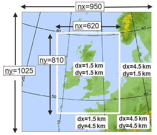
The functions that are used to include the effects of stability on turbulence, via the Richardson number (Ri), follow Brown
     (1999):
                                                               1               1/2
     fm = (1 − cLEM Ri)1/2                            fh =        (1 − bLEM Ri)                                                      (1)
                                                             P rN
5    where P rN is the neutral Prandtl number (= 0.7). In RAL0, the constants bLEM and cLEM are both equal to 1.43 (which gives
     Brown’s “conventional” model). RAL0 uses a mixing length that is a fraction (0.15) of the depth of any layer where Ri less
     than a critical value (Ricrit = 0.25), within that layer, or 40m if larger.
       In an effort to improve the triggering of explicit convection, stochastic perturbations to temperature are applied. Designed
     to represent realistic variability that might be seen due to large boundary layer eddies, the perturbation scale for potential
10   temperature, θ, is taken as θ∗ = w0 θ0 |s /wm , where w0 θ0 |s is the surface turbulent flux of θ and the turbulence velocity scale
                     3
     wm is given by wm = u3∗ + cws w∗3 . Here u∗ is the friction velocity and w∗ the convective velocity scale, with cws = 0.25.
     Finally θ∗ is constrained to be positive and less than 1 K. Loosely based on Munoz-Esparza et al. (2014), the random number
     field that multiplies the perturbation scale is held constant over 8 grid-length squares in the horizontal and the perturbations are
     applied uniformly in the vertical up to the lower of two-thirds of the boundary layer depth and 400m.

15   2.8   Land surface and hydrology

     Exchanges of mass, momentum and energy between the atmosphere and the underlying land and sea surfaces are represented
     using the community land surface model JULES (Best et al., 2011; Clark et al., 2011). The configuration adopted in RAL0
     largely follows that of GL7.0, as described by (Walters et al., 2017). In keeping with the seamless approach to model devel-
     opment, the aim is to minimize the differences between configurations, but different developmental priorities for regional and
20   global modelling can result in differences between the configurations, even if there is no compelling scientific motivation to
     maintain them. We now list and explain the non-trivial differences.
       Because the UKV was developed for short-range forecasting over the UK, the treatment of surface exchange over sea and
     sea ice has been less of a priority than in the global model, so that RAL0 is less advanced in its treatment. A fixed value of
     Charnock’s coefficient (0.011) is used to determine the surface roughness over open sea, as opposed to the COARE algorithm
25   in GL7.0. GL7.0 also includes a more advanced parametrisation of the sea surface albedo (Jin et al., 2011) that incorporates a
     dependence on the wind speed and chlorophyll concentration. This has not yet been introduced into RAL0, which still uses an
     earlier scheme based on Barker and Li (1995). Similarly, because the regional model has not yet been used operationally over
     sea ice, several recent modifications to sea-ice parameters have not yet been introduced into the regional configuration. Sea-ice
     is not present in the simulations shown below, so these settings are not relevant to any results presented here.
30     Although both GL7.0 and RAL0 include the multilayer snow scheme, different densities of fresh snow are specified: in
     GL7.0 the value is 109 kgm−3 , while in RAL0 a value of 170 kgm−3 is used as more representative of the conditions in the
     UK. In the future, it is hoped that it will be possible to relate the density to local meteorological conditions.
       Both GL7.0 and RAL0 represent the radiative transfer in plant canopies using the two-stream radiation scheme of Sellers
     (1985), with the leaf-level reflection and transmission coefficients presented in that paper. However, in GL7.0, an adjustment to

                                                                       9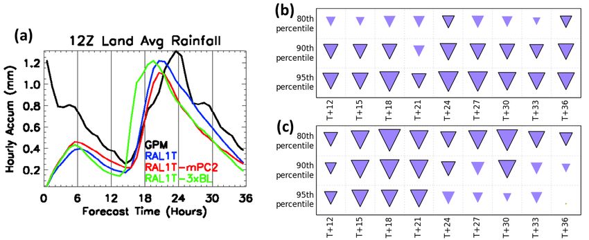
these parameters is made as the model runs to make the grid-box mean albedo agree more closely with a climatology derived
     from GlobAlbedo. While developing this adjustment for GL7.0, the simulated direct albedos were found to be unrealistic and
     the diffuse albedos were used for both the direct and diffuse beams. As implemented in RAL0, there is no adjustment to a
5    climatology and both the direct and diffuse albedos are used. Further discussion of these issues may be found in section 3.5.
       Two differences in soil hydrology should be noted. Whereas the more elaborate TOPMODEL scheme is used to represent
     soil moisture heterogeneity in GL7.0, the simpler PDM scheme is used in RAL0 (consult Best et al. (2011) for details of these
     schemes). Also, in RAL0, if the simulated soil moisture rises above the saturated water content, the excess is assumed to move
     upwards and to contribute to surface runoff. This is considered more realistic than the alternative of routing the excess moisture
10   downwards, except in regions of partially frozen soils (Best et al., 2011). Therefore, in GL7.0 the excess moisture is routed
     downwards.
       In GL7.0 urban surfaces are represented by a single urban tile, but in RAL0 two separate tiles for street canyons and roofs
     are used (Porson et al., 2010). Currently the two tile scheme is limited to domains over the UK due to the availability of
     morphology data.

15   2.9    Lower boundary condition (ancillary files) and forcing data

     In the UM, the characteristics of the lower boundary, the values of climatological fields and the distribution of natural and
     anthropogenic emissions are specified using ancillary files. Use of correct ancillary file inputs can potentially play as important
     a role in the performance of a system as the correct choice of many options in the parametrisations described above. In the
     future we may consider the source data and processing required to create ancillaries as part of the definition of the RAL
20   configurations as is the case in global configurations. However we currently leave ancillaries outside the formal definition of
     RAL as there has been no systematic evaluation of the impact on performance of different ancillary file inputs and the existence
     of many country specific datasets (that are of better quality or higher resolution) mean that different applications (especially
     operational ones such as UKV/MOGREPS-UK) use different source datasets, sometimes even combining different datasets
     within the model domain. An example of this is described in section 3.5.
25     Table 4 in the appendix contains the main ancillaries used in RAL applications as well as references to the source data from
     which they are created.

     2.10    Other differences from GA7 due to horizontal resolution

     The high horizontal resolutions used for RAL simulations mean that RAL0 runs with the convection parametrisation switched
     off, relying on the model dynamics to explictly represent convective clouds. Although it is acknowledged that not all types of
     convection are represented with such grid-spacing, this choice was made in the current absence of a scale-aware convection
     scheme which correctly parametrizes sub-grid convective motion and hands over to the model dynamics for clouds larger than
     the model filter scale. Projects are underway to develop convection schemes for use in atmospheric models at all resolutions
     with grid spacings O(1–100,km), which could be incorporated into a future RAL release.

                                                                     10
5 Also, RAL0 does not include a sub-grid parametrisation scheme for either orographic or non-orographically forced gravity
waves. However for those non-UK-area models that run with a grid-length of 0.04 ◦ (4.4 km), the inclusion of the effective
roughness and gravity wave drag schemes (both as used in GA7) was found to be beneficial to near-surface verification scores.
3 Developments included in RAL1
This section describes the RAL1-M developments which when added to the RAL0 base define RAL1-M. The Regional Model
10 Evaluation and Development (RMED) processes at the Met Office makes use of an online ’ticket’ tracking system which allows
scientists to document changes to the model. A ticket number is assigned to each model development and thus it is clear to
all developers and external collaborators which tickets are included in any one configuration. In this section we discuss the
major developments to RAL1 and reference them by ticket number to inform both the development community and for future
cross-reference.
15 3.1 Dynamical formulation and discretisation
Conservative advection for moist prognostics (RMED ticket #2)
The mass conservation for mixing-ratios is achieved with the ZLF (Zero-Lateral-Flux) scheme (Zerroukat and Shipway, 2017).
This scheme is computationally efficient and exploits the relatively large width of LBCs used for semi-Lagrangian based LAMs
(i.e., the size of the extra extended computational zone ΩE = Ω2 + Ω3 + Ω4 shown in Figure 1). Assuming that the size of ΩE
20 is sufficiently large (> 2 points) it can be divided into two regions as shown in Figure 1 with a dotted line/boundary Γ2 , which
will be referred as the ZLF boundary. It is also very common that the wind and the time step used are such that the horizontal
Courant number in the RIM zone is smaller than half of the RIM size. Under these conditions, the SL advection solution for all
the points inside the region {Ω1 + Ω2 } (which includes the forecasting zone) will be unaffected by the field beyond the ZLF
boundary Γ2 . Therefore, for convenience, the advection solves a modified problem, whereby inside Γ2 the advected quantity
25 is the original field, whereas the field beyond Γ2 is zeroed. This modification does not affect the solution inside the domain
{Ω1 + Ω2 } and hence it is equivalent to the original problem. However, this modification allows us to impose a simple mass
conservation constraint over the whole extended computational domain {Ω1 + Ω2 + Ω3 } where there is no need to compute
lateral fluxes because they are zero by construction (see details in Zerroukat and Shipway (2017)). This is quite an important
simplification from the case where one would like to impose a mass conservation budget for the forecast/physical domain
30 Ω1 , which requires knowledge of mass fluxes through its lateral boundary Γ1 , which are complicated and computationally
expensive to compute (Aranami et al., 2014). The ZLF scheme has two components: the first part (just explained above) which
allows us to avoid computing expensive lateral fluxes, while the second part is the redistribution of the mass conservation error
using the optimized conservation scheme (Zerroukat and Allen, 2015). Note that the zeroing is just an intermediate temporary
step used during the advection, because the zeroed-region gets overwritten by the appropriate LBC data at the end of the time
step.
115 3.2 Solar and terrestrial radiation
Improved treatment of gaseous absorption (RMED ticket #9)
The treatment of gaseous absorption has been significantly updated to the configuration used with GA7 (Walters et al., 2017).
Forty-one (41) k terms are used for the major gases in the SW bands with an improved representation of H2 O, CO2 , O3 , and
O2 absorption and the addition of absorption from nitrous oxide (N2 O) and methane (CH4 ). These changes result in increased
10 atmospheric absorption and reduced surface (clear-sky) fluxes.
Eighty-one (81) k terms are used for the major gases in the LW bands with an improved representation of all gases. This
results in reduced clear-sky outgoing LW radiation, and increased downwards surface fluxes.
The method of “hybrid” scattering is used in the LW which runs full scattering calculations for 27 of the major gas k-terms
(where their nominal optical depth is less than 10 in a mid-latitude summer atmosphere). For the remaining 54 k-terms (optical
15 depth > 10) much cheaper non-scattering calculations are run.
In both spectral regions the band-by-band breakdown of absorption is improved which should improve interaction with
band-by-band aerosol and cloud forcing.
3.3 Microphysics
Improved droplet number profile in the lower boundary layer (RMED ticket #1)
20 Previous work by Wilkinson et al. (2013) had discussed a pragmatic method of reducing the cloud droplet number near the
surface, often referred to as a “droplet taper”. This reduction accounts for the fact that aerosol activation and cloud droplet
numbers measured in fog are often much lower than those found in more elevated clouds, despite the fact that the underlying
aerosol concentrations are generally higher. Recent work by Boutle et al. (2018) utilising new observations (Price et al., 2018)
has enhanced our understanding of this process, demonstrating that weak updraughts and low supersaturations in fog are the
25 reason for the limited aerosol activation. Boutle et al. (2018) showed that even the droplet number profile of Wilkinson et al.
(2013) gave values too high too close to the surface. This triggered a feedback process whereby fog became too deep and well-
developed too quickly, resulting in significant errors to fog forecasts. Boutle et al. (2018) proposed a modified parametrisation
for the near-surface droplet number, which was shown in forecast trials to be of significant benefit. Therefore RAL1 has adopted
the droplet number parametrisation proposed by Boutle et al. (2018), i.e. droplet numbers are held at 50 cm−3 throughout the
lowest 50 m of the atmosphere, before transitioning to the cloudy values as described in Wilkinson et al. (2013). We note that
this is still a pragmatic choice based on model performance, and further work is required to develop an activation scheme which
correctly accounts for aerosol effects and is valid in the foggy regime.
125 3.4 Atmospheric Boundary Layer
Updates to stochastic boundary layer perturbations (RMED ticket #25)
Several updates were made to the stochastic perturbations in the boundary layer (described in section 2.7) for RAL1 in order to
further enhance the triggering of convective activity. The first was also to apply the perturbations to specific humidity, using the
same formulation for the perturbation scale (based on the surface humidity flux), constraining the moisture scale to be less than
10 10% of the specific humidity itself. Secondly the random number field was changed from being randomly different every time
step to being updated in time following McCabe et al. (2016) using a first-order auto-regression model with the auto-correlation
coefficient set to give a decorrelation timescale of 600 s, an approximate eddy-turnover timescale. This temporal coherence of
the perturbations results in a greater resolved scale dynamical response. Finally, in the vertical the perturbations are now scaled
by a piece-wise linear “shape” function equal to unity in the middle of the boundary layer and zero at the surface and top of
15 the sub-cloud layer. This was a pragmatic change to avoid the perturbations strongly influencing the screen-level temperature
diagnostic, which had been found to lead to degradation of deterministic measures of skill (such a root-mean-square error).
Revision of free-atmospheric mixing length (RMED ticket #12)
In RAL1-M, the free-tropospheric (i.e., above the boundary layer) mixing length is reduced everywhere to its minimum value
of 40m, which was found to give better, more rapid initiation of showers in UKV than the interactive mixing length used in
20 RAL0 (and also kept for RAL1-T, see section 4).
Improved representation of mixing across the boundary layer top (RMED ticket #5)
This ticket allows the boundary layer scheme’s explicit entrainment parametrisation to be distributed over a vertically-resolved
inversion layer, instead of always assuming the inversion to be subgrid. As a result it allows a smoother transition in the vertical
between the boundary layer and free troposphere. More details are given in Walters et al. (2017) (under GA ticket #83), noting
25 that the additional representation of “forced cumulus clouds” within a resolved inversion is only included in RAL1-T (see
section 4) as that requires the PC2 cloud scheme to be used.
Reductions in sensitivity to vertical resolution (RMED ticket #10)
The turbulent mixing and entrainment in cloud-capped boundary layers in the Lock et al. (2000) scheme is parametrized
in terms of (among other things) the strength of cloud-top radiative cooling. This is calculated by differencing the radiative
flux across the top grid-levels of the cloud layer. The complexity of the calculation is increased by making allowance for
changes in the height of cloud between radiation calculations (which are not performed on every model time step for reasons of
computational efficiency). A new methodology is introduced that identifies where the LW radiative cooling profile transitions
from free-tropospheric rates above the cloud to stronger rates within it. It has very little impact at current vertical resolutions
135 (typically greater than 100m) but has been demonstrated in the single column version of the model to be robustly resolution
independent down to grids of only a few metres.
3.5 Land surface and hydrology
Improvements to land usage and vegetation properties (RMED ticket #3)
There are four changes to the representation of the land surface in RAL1:
10 1. updated land use mappings, mainly removing small (too late or not at all. In order to cope with this, RAL1-M, has several aspects of its configuration to encourage the model fields
to be less uniform and help convection initiate, namely stochastic perturbations and relatively weak turbulent mixing. If the
model is run with these in the tropics the model initiates too early and convective cells tend to be too small. For this reason,
5 there are two differences in the representation of turbulence between RAL1-M and RAL1-T, namely in the form of the stability
functions (the (Brown, 1999) “standard” model is used, with bLEM = 40, cLEM = 16) and in the free-atmospheric mixing
length (which retains RAL0’s interactive one). Both give enhanced turbulent mixing in RAL1-T compared to RA1-M. The
other related change is that the stochastic boundary layer perturbations are not used in RAL1-T.
A related difference is that RAL1-T has three extra prognostic fields (liquid fraction, ice fraction and mixed-phase fraction) as
10 it uses the prognostic cloud prognostic condensate (PC2) cloud scheme (Wilson et al., 2008a). PC2 calculates sources and sinks
of cloud cover and condensate and advects the updated cloud fields, hence adding some memory into the system. One advantage
of PC2 over the Smith schemes is the looser coupling between variables, hence allowing a cloud to deplete its liquid water
content while maintaining high cloud cover. The PC2 scheme performs better than the Smith scheme in climate simulations
(Wilson et al., 2008b) and for global numerical weather prediction (Morcrette et al., 2012). It is worth noting that when run
15 in a model using a convection scheme, the detrainment of cloud from convection is a key source of cloudiness (Morcrette and
Petch, 2010; Morcrette, 2012b). When run in a model without a convection scheme (such as the RAL configuration), cloud
formation from convective motions will be represented by a combination of PC2 initialization (near convective cloud base),
followed by PC2 pressure forcing through the rest of the updraught. In the PC2 scheme, cloud erosion is a process that accounts
for evaporation and reduction of cloud cover due to unresolved mixing near cloud edges. In the original implementation of PC2
20 (Wilson et al., 2008a) erosion was carried out as part of the call to the convection scheme, but in RAL1, which has no call
to the convection scheme, the erosion process has been moved to occur within the microphyics scheme. In RAL1-T, the PC2
scheme is implemented as in the GA7 global model configuration (Walters et al., 2017). That is, the formulation of cloud
erosion accounts for the apparent randomness of cloud fields, as described in Morcrette (2012a) and the RHcrit is calculated
from the turbulent kinetic energy (Van Weverberg et al., 2016).
Another difference, particularly affecting convection in the tropics, is that the tropopause is deeper than in mid-latitudes. In
order to take account of this RAL1-T uses a vertical level set labelled L80(59t;21s)38:5, which adds some additional vertical
resolution in the tropical upper-troposphere at the expense of resolution in the lower boundary layer.
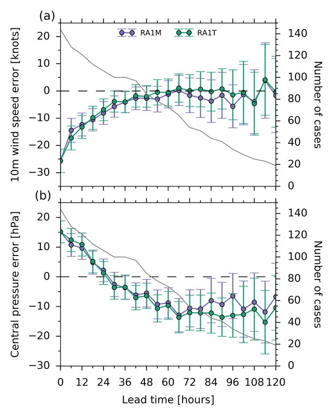
Figure 2 illustrates the above discussion by showing the effect of running RAL1-M and T for a case of small showers in
5 the U.K. Unlike RAL1-M, when compared to the radar RAL1-T initiates too late and produces too large and too few showers.
Table 2 contains a summary of differences between RAL1-M and RAL1-T for the convenience of the reader.
5 Model evaluation
In this section we apply a range of evaluation methods to demonstrate the performance of RAL1. The regional model evaluation
process is rapidly evolving and has already benefitted from the multi-institutional UM partnership. The regional model is run
15Table 2. RAL1-M and RAL1-T differences. %
Science difference RAL1-M RAL1-T
Cloud Scheme Smith (diagnostic) PC2 (prognostic)
BL Free Atmospheric mixing length 40m interactive mixing lenth (enhancement to turbulent mixing)
BL Stability functions bLEM =1.43, cLEM =1.43 bLEM =40, cLEM =16 (enhancement to turbulent mixing)
BL stochastic perturbations to temperature and moisture on (improved triggering) off
10 by UM partners in a variety of domains worldwide and RAL1 marks a baseline to which all centres can now focus future
evaluation effort.
In this first documentation of the regional model we have focused on performance of RAL1 over the UK, Singapore, Aus-
tralia, the Western North Pacific (Philippine Area of Responsibility for Tropical Cyclone forecasting) and the USA. This allows
inspection of model behaviour in a variety of climatic zones and for different weather phenomena.
15 A range of evaluation methods are required to assess the performance of models. Verification skill scores, anomaly plots and
case studies all provide useful information which builds a picture of model characteristics and skill. Kilometre scale models
behave and look differently to models where the convection is parameterised. Convection in these models is more likely to
look realistic than in a global (parameterised) model and may mimic many of the characteristics seen in satellite images and
animations. However, although the detail looks realistic, it may not always be skilful. It is a challenge to create metrics which
20 can truthfully represent the benefit of kilometre scale models as well as clarify their limitations.
Mittermaier (2014) proposed a new spatial and inherently probabilistic framework for evaluating kilometre scale models
and Mittermaier and Csima (2017) provide a historical overview of performance of the 1.5 km model using this new “High
Resolution Assessment” (HiRA) framework. The framework uses synoptic observations, but instead of using the single nearest
model grid point, it uses a neighbourhood of model grid points centered on the observing location to acknowledge the fact
25 that added detail may not be in the right place at the right time. These points can be treated as a pseudo ensemble, and we can
compute ensemble metrics as it can be assumed that all the forecast values in the neighbourhood are equally likely outcomes
at the observing location. One caveat to ensure this assumption holds is that the neighbourhood most not be too large. The
framework can be applied to deterministic and ensemble forecasts, including the control member of the ensemble. Whilst it
may be less than intuitive to think that a forecast neighbourhood is required for temperature, it was shown in Mittermaier and
30 Csima (2017) that all variables benefited from the use of at least a 3 x 3 neighbourhood, but that too large neighbourhoods may
be detrimental for some variables, including temperature. The HiRA Ranked Probability Score (RPS) is used for non-normally
distributed or spatially discrete variables whilst the Continuous Ranked Probability Score (CRPS) is used for temperature.
The Fractions Skill Score (FSS, Roberts and Lean, 2008) requires spatial observation-based analysis. Over the UK this is
a radar-based analysis, though more recently a GPM based product (Skofronick-Jackson et al., 2017) has also been used for
evaluating kilometre grid scale configurations in the tropics. Analyses based on remote-sensed data and may not be accurate in
16an absolute sense (no observations are perfect and error-free). The FSS is sensitive to the bias (Mittermaier and Roberts, 2010),
and for this reason the FSS is generally used in conjunction with percentile thresholds, where all the values in the forecast
5 and analysis domains are ranked separately, and the physical value associated with a specific centile is extracted. This quantile
transformation removes the bias so that the FSS based on percentile thresholds offers a measure of field texture, pattern and
areal extent, and not intensity.
5.1 Introducing the RMED “toolbox”
To assist the RMED processes, an evaluation toolbox has been created to support model development. The main purpose is
10 to ensure a uniformity of verification and diagnostic output across multiple users and institutions. Version 1 of the toolbox
was released in time for the RAL1 assessment. It contains a selection of verification techniques and diagnostic tools, intent
on enabling the comparison with point observations as well as gridded truth sources. One of the outputs of the toolbox is a
‘scorecard’ - a single clear plot with arrows/triangles showing whether the model version being tested is better or worse than a
previous incarnation. The size of the triangles signal the improvement (or deterioration) strength and the triangles are outlined
15 in black if the change is statistically significant. The scorecards contain a huge amount of information, digested into an easy-
to-understand summary. This allows fast assessments about model skill to be made, speeding up the evaluation (and therefore
development) process. The model verification plotting comprises the FSS (score with spatial scale, score with forecast lead
time, accumulation equivalent to particular centile with forecast lead time) and HiRA scores including bias at neighbourhood
size with forecast lead time. Plotting of more traditional metrics (e.g. mean error and root-mean-square error (RMSE) at a grid
20 point) was also included for a range of parameters (surface temperature, wind, relative humidity and 6-hourly precipitation
amounts).
The diagnostic methods implemented in RMED toolbox version 1 also included domain (area) average plots (for a compre-
hensive set of meteorological diagnostics) especially useful for considering the diurnal cycle, histograms (for parameters such
as screen temperature, wind, 3h mean rain rates and outgoing longwave radiation) for exploring distributions, and “cell statis-
25 tics” (Hanley et al., 2015), a method for investigating the texture of a field through the application of a threshold to identify
areas of exceedance or “cells”. The number and size of the cells can then be analysed. This was first implemented to compare
3-hour mean rain rates against GPM IMERG satellite data (Huffman, 2015, 2017), or if appropriate, UK radar data. The ability
to create charts of model fields for a specific set of meteorological variables was also provided.
RAL1 provides a lot of detail due to its use at high resolution, but this can increase noise in traditional verification measures
30 such as the root-mean-square error, which favours smooth fields over noisy ones. Multiple scores for the same parameter can be
a source of confusion, providing different, even contradictory results. The RPS and FSS both evaluate hourly precipitation but
they measure different attributes of the precipitation forecast. The FSS scores measures pattern, and the HiRA RPS focuses on
intensity. It is possible to improve the forecast intensities whilst degrading the spatial pattern or texture of the forecast and this
can lead to difficult to interpret verification scores. Murphy and Winkler (1987) stated the need for more than one independent
score, measuring a range of forecast attributes to get a robust perspective of forecast performance.
175.2 Mid-Latitude performance over the UK
In this section we illustrate the impact of the RAL1 changes on model performance. The baseline used for the UK and mid-
latitudes is RAL0. The UK evaluation consisted of running 100 case studies run with a 1.5km horizontal grid-length, using
5 the same domain as the Operational UKV model (Figure 3). The cases sampled a wide range of meteorological conditions
from the period July 2014 to April 2017 and comprised roughly equal numbers from each season. The model runs were simple
downscaling runs with no data assimilation from a mixture of 00Z and 12Z runs of the Met Office Global model. To test the
impact of including data assimilation in RAL1, one month long Summer and Winter 2016 UKV 3D-VAR Data Assimilation
trials were then carried out.
10 The HiRA scorecards for the 100 case studies along with the 3D-Var trials are shown in figure 4 and figure 5 , these show
the performance of RAL1 compared to RAL0. One of the most significant improvements in RAL1 is the surface temperature.
Figure 6 shows the diurnal cycle of 1.5m temperature bias and RMSE for RAL1-M and RAL1-T against RAL0 for the 100
case studies. The figure shows that RAL1 reduces the bias and RMSE in the diurnal cycle of screen temperature. This addresses
a long standing problem in the UKV model and is reflected in a statistically significant improvement to the Temperature RPS
15 at most lead times in both case study (Figure 4, top row) and 3D-Var trials (Figure 5, top row). The improvement is primarily
because of an increase in vegetation cover, at the expense of bare soil in RAL1, that reduces the thermal coupling between
the atmosphere and soil. The reduction in scalar roughness lengths over grass tiles enhances the difference between skin and
air temperatures. These changes lead to an amplified diurnal cycle of screen temperature and are supported by observational
studies at the Met Office Research Unit site at Cardington, near Bedford.
20 The albedos of vegetated tiles are also reduced in RAL1 and this results in warmer daytime temperatures. These changes
were all components of ticket 3 (see section 3.5). The impact on screen temperature varies according to the amount of vegetation
present at a particular location. This is clearly illustrated by temperature differences over the UK shown in figure 7. In these
plots the imprint of urban areas such as London show up as an area of little change between model versions RAL0 and RAL1.
Another impact of the increase in vegetation cover from ticket 3 is that RAL1 reduces wind speeds (through an increase in the
25 roughness length and therefore surface drag). The reduced wind speeds are beneficial at night time (reducing an overforecasting
bias), but detrimental by day (Figure 8). Overall RAL1 shows statistically significant improvement to the 10m wind RPS at
most lead times in both case study (Figure 4) and 3D-Var trials (Figure 5).
RAL1 gives an improvement to precipitation RPS at most lead times as seen in both case studies (Figure 4) and 3D-
Var Summer trial (Figure 5 right panel). The 3D-Var Winter trial shows even stronger benefit with statistically significant
30 improvements at all lead times (Figure 5 left panel). These HiRA results are based on raingauge data. 1hr FSS results (based
on UK. radar as truth) for the case studies (Figure 10) show improvements to the 90th and 95th percentile results at all forecast
ranges. The percentiles contain no bias information. However the absolute thresholds at 0.5mm, 1.0mm and 4.0mm in the
hour generally show a detriment. The 6hr FSS for the case studies (Figure 11) show similar results and point to potentially
undesirable changes to bias. The overall Precipitation Mean Error in the case studies is reduced in RAL1-M and this reduces
an overforecasting bias (now shown). The 1mm frequency bias and 4mm frequency bias results (not shown) indicate that as
18You can also read