ATMOSWING: ANALOG TECHNIQUE MODEL FOR STATISTICAL WEATHER FORECASTING AND DOWNSCALING (V2.1.0) - GMD
←
→
Page content transcription
If your browser does not render page correctly, please read the page content below
Geosci. Model Dev., 12, 2915–2940, 2019
https://doi.org/10.5194/gmd-12-2915-2019
© Author(s) 2019. This work is distributed under
the Creative Commons Attribution 4.0 License.

AtmoSwing: Analog Technique Model for Statistical Weather
forecastING and downscalING (v2.1.0)
Pascal Horton1,2,3
1 Universityof Bern, Oeschger Centre for Climate Change Research, Institute of Geography, Bern, Switzerland
2 Universityof Lausanne, Institute of Earth Sciences, Lausanne, Switzerland
3 Terranum SARL, Bussigny, Switzerland

Correspondence: Pascal Horton (pascal.horton@giub.unibe.ch)

Received: 15 February 2019 – Discussion started: 28 March 2019
Revised: 4 June 2019 – Accepted: 17 June 2019 – Published: 12 July 2019

Abstract. Analog methods (AMs) use synoptic-scale predic-           change impact studies. When used for future climate studies,
tors to search in the past for similar days to a target day in      it is necessary to pay close attention to the selected predictors
order to infer the predictand of interest, such as daily precipi-   so that they contain the climate change signal.
tation. They can rely on outputs of numerical weather predic-           The Optimizer implements different optimization tech-
tion (NWP) models in the context of operational forecasting         niques, such as a semiautomatic sequential approach, Monte
or outputs of climate models in the context of climate im-          Carlo simulations, and a global optimization technique, us-
pact studies. AMs require low computing capacity and have           ing genetic algorithms. Establishing a statistical relationship
demonstrated useful potential for application in several con-       between predictors and predictands is computationally inten-
texts.                                                              sive because it requires numerous assessments over decades.
   AtmoSwing is open-source software written in C++ that            To this end, the code was highly optimized for computing ef-
implements AMs in a flexible way so that different variants         ficiency, is parallelized (using multiple threads), and scales
can be handled dynamically. It comprises four tools: a Fore-        well on a Linux cluster. This procedure is only required to
caster for use in operational forecasting, a Viewer to display      establish the statistical relationship, which can then be used
the results, a Downscaler for climate studies, and an Opti-         for forecasting or downscaling at a low computing cost.
mizer to establish the relationship between predictands and
predictors.
   The Forecaster handles every required processing inter-
nally, such as NWP output downloading (when possible) and           1   Introduction
reading as well as grid interpolation, without external scripts
or file conversion. The processing of a forecast requires low       Approaches based on the concept of analogy are widespread
computing efforts and can even run on a Raspberry Pi com-           in different domains of science and engineering. In hydrom-
puter. It provides valuable results, as revealed by a 3-year-       eteorology, it entails retrieving data on atmospheric condi-
long operational forecast in the Swiss Alps.                        tions from the past that can be considered similar to the sit-
   The Viewer displays the forecasts in an interactive GIS en-      uation at hand, with consequences that may be expected to
vironment with several levels of synthesis and detail. This         be similar. The consequences can be local variables of inter-
allows for the provision of a quick overview of the potential       est such as the occurrence of fog, favorable conditions for
critical situations in the upcoming days, as well as the pos-       avalanches, wind intensity, or the precipitation amount. The
sibility for the user to delve into the details of the forecasted   approach relies on the idea expressed by Lorenz (1956, 1969)
predictand and criteria distributions.                              that similar situations in terms of atmospheric circulation are
   The Downscaler allows for the use of AMs in a cli-               likely to lead to similar local weather. AMs require at least
matic context, either for climate reconstruction or for climate     two concurrent archives: one that provides the value of the
                                                                    local variable of interest, called the predictand, and another

Published by Copernicus Publications on behalf of the European Geosciences Union.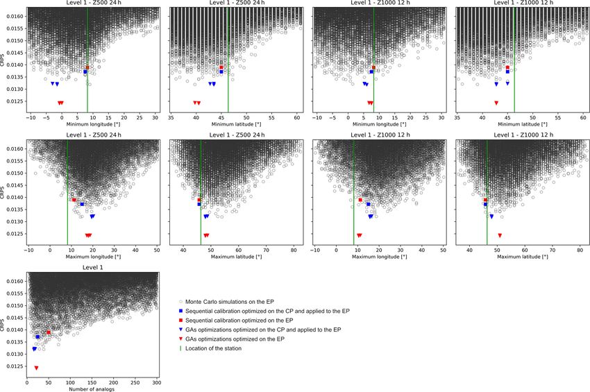
2916                                                                                                       P. Horton: AtmoSwing

one describing the past atmospheric situations, through dif-       most useful techniques for daily precipitation (Maheras et al.,
ferent variables called predictors, to which the situation at      2005; Schmidli et al., 2007). Bliefernicht (2010) obtained
hand will be compared.                                             more superior results with AMs than downscaling methods
   Usually, the predictand values can be derived by model-         based on weather typing.
ing the chain of processes linking the predictors to the pre-          The use of AMs for the operational forecasting of daily
dictand. The processes involved range from large-scale dy-         precipitation originates in the work of Duband (1970, 1974,
namical states of the atmosphere down to very small-scale          1981). They were then designed for operational forecasting
microphysical processes. These require models that are ex-         at EDF (Électricité de France) in order to better manage wa-
tremely complex, data intensive, and time-consuming. Con-          ter resources and flood risks. They are used mainly by practi-
versely, given an appropriate set of predictor archives, a suf-    tioners, notably hydropower companies (Desaint et al., 2008;
ficient number of situations analogous to a target situation       Ben Daoud et al., 2009; Obled, 2014) and flood forecast-
can be identified so that reasonable values can be obtained        ing services in France and Switzerland (Marty, 2010; Gar-
for the predictand with low computing effort. This is particu-     cía Hernández et al., 2009; Horton et al., 2012). When com-
larly true for a specific predictand that is critical in hydrom-   paring the results from AMs to an ensemble forecast, Marty
eteorological applications, namely the precipitation amount        (2010) found AMs to be better than the considered ensemble,
over a given domain and time duration. The forecast pro-           particularly for strong precipitation. However, AMs should
vided by AMs is issued as a statistical distribution based on      not be considered as a substitute for NWP models but as a
the observed predictand values from the selected analogs un-       complement in order to obtain a fast statistical adaptation that
less only the single best analog is considered, which usually      is known to be accurate several days in advance. Therefore,
results in a lower skill (Bontron and Obled, 2005).                they contribute to the analysis of potentially critical situa-
   Analog methods (AMs) are used in two different types            tions in flood forecasting, for example, and are very useful in
of approaches (Rummukainen, 1997): perfect prognosis, for          early warning.
which the statistical relationship is calibrated using observed        Hamill and Whitaker (2006) used an analogy-based ap-
predictors, and model output statistics (MOS), for which           proach on the Global Forecast System (GFS) reforecasts in
the relationship is calibrated using outputs of a specific cli-    order to correct systematic errors in the ensemble forecasts of
mate or numerical weather prediction (NWP) model. AMs              temperature and precipitation. These biases were corrected
are often used to predict daily precipitation, either in an op-    by taking into account the intrinsic local climatology pro-
erational forecasting context (e.g., Guilbaud, 1997; Bontron       vided by the AM. Moreover, the under-dispersion of the en-
and Obled, 2005; Hamill and Whitaker, 2006; Bliefernicht,          semble forecast from the numerical model has also been cor-
2010; Marty et al., 2012; Horton et al., 2012; Hamill et al.,      rected using analogs (Hamill and Whitaker, 2006). The cor-
2015; Ben Daoud et al., 2016) or a climate downscaling con-        rection of ensemble forecast under-dispersion using AMs is
text (e.g., Zorita and von Storch, 1999; Wetterhall, 2005;         also used operationally at EDF (Électricité de France).
Wetterhall et al., 2007; Matulla et al., 2007; Radanovics              The present work does not introduce a new method, but it
et al., 2013; Chardon et al., 2014; Dayon et al., 2015; Ray-       introduces software called AtmoSwing that implements AMs
naud et al., 2016). Other predictands are also considered,         in a versatile and efficient way. It is versatile in that it facili-
such as precipitation radar images (Panziera et al., 2011;         tates the building of AM structures in a dynamic way and be-
Foresti et al., 2015), temperature (Radinovic, 1975; Wood-         cause the code is written with an object-oriented architecture.
cock, 1980; Kruizinga and Murphy, 1983; Delle Monache              It is efficient because it is written in C++ and leverages paral-
et al., 2013; Caillouet et al., 2016; Raynaud et al., 2016),       lel computing. AtmoSwing is made up of different modules
wind (Gordon, 1987; Delle Monache et al., 2013, 2011; Van-         targeted either for operational forecasting (the Forecaster and
vyve et al., 2015; Alessandrini et al., 2015b; Junk et al.,        the Viewer) or for climate impact studies (the Downscaler).
2015b, a), solar radiation or power production (Alessandrini       Additionally, a module (the Optimizer) is available for cali-
et al., 2015a; Bessa et al., 2015; Raynaud et al., 2016), snow     brating the different parameters of the method. AtmoSwing
avalanches (Obled and Good, 1980; Bolognesi, 1993), and            is continuously evolving and has been used in Horton et al.
the trajectory of tropical cyclones (Keenan and Woodcock,          (2012, 2017a, b, 2018) and Horton and Brönnimann (2018).
1981; Sievers et al., 2000; Fraedrich et al., 2003). AMs are           Some existing AMs designed for daily precipitation will
also used for seasonal forecast (Barnston et al., 1994; Xavier     first be described along with the required data (Sect. 2), and
and Goswami, 2007; Charles et al., 2012; Wu et al., 2012;          the software will then be presented (Sect. 3) together with
Shao and Li, 2013).                                                the details of the modules: the Forecaster (Sect. 3.3), the
   An AM was evaluated during the project STARDEX                  Viewer (Sect. 3.4), the Downscaler (Sect. 3.5), and the Op-
(STAtistical and Regional dynamical Downscaling of                 timizer (Sect. 3.6). Section 4 discusses the parameter space
EXtremes for European regions; see Goodess, 2003;                  of AMs through different calibration techniques, and Sect. 5
STARDEX, 2005). One of the goals of the project was to             provides feedback from operational precipitation forecasting
compare various downscaling methods to determine weather           in the Swiss Alps. Some limitations of the AM are discussed
extremes, and the AM was selected as being among the

Geosci. Model Dev., 12, 2915–2940, 2019                                               www.geosci-model-dev.net/12/2915/2019/
P. Horton: AtmoSwing                                                                                                         2917

in Sect. 6. The conclusions (Sect. 7) provide some additional     comparison Project Phase 5 (CMIP5; Taylor et al., 2012) and
perspectives for future developments of AtmoSwing.                EURO-CORDEX (Jacob et al., 2014).

                                                                  2.2     Analog methods for daily precipitation
2     Data and methods
                                                                  AtmoSwing does not rely on a single structure of the AM but
2.1    Required data                                              can implement different variants. A non-exhaustive selection
                                                                  of methods developed for different regions will be presented
AMs generally require three datasets: the historical predic-      hereafter, focusing on the prediction of daily precipitation.
tand values, the historical predictor values for the same pe-
riod, and the predictors describing the target situation.         2.2.1    Characteristics of the AM
   The predictand is often a daily or 6-hourly time series. One
                                                                  Definition of the analogy. The AM is based on the principle
of the most used predictands is daily precipitation, which is
                                                                  that two similar synoptic situations may produce similar lo-
usually averaged over subregions in order to smooth local
                                                                  cal effects (Lorenz, 1956, 1969). The perfect analogy does
effects (Obled et al., 2002; Marty et al., 2012). These time
                                                                  not exist, but sufficiently similar situations leading to similar
series can be normalized by the precipitation value for a cer-
                                                                  effects can be identified. To be relevant, this analogy must be
tain return period (for example, 10 years; Djerboua, 2001) to
                                                                  selected by optimizing the following elements.
allow for an easier comparison between subregions subject
to different precipitation regimes.                                 – The meteorological variables (predictors) must contain
   In the early days of AMs in operational forecasting, the           synoptic-scale information with a direct or indirect de-
predictors were based on radio-sounding data. Nowadays,               pendency on the target predictand.
the predictor archive is often a global atmospheric reanalysis
dataset, which provides gridded large-scale variables at any        – The pressure (or isentropic) levels at which the predic-
location in the world. Reanalyses are produced using a single         tors are selected must be determined.
version of a data assimilation system coupled with a forecast
model constrained to follow observations over a long period.        – The spatial windows are the domains over which pre-
They provide multivariate outputs that are physically con-            dictors are compared.
sistent, which contain information on locations where few
or no observations are available, including variables that are      – The temporal windows are the hours of the day at which
not directly observed (Gelaro et al., 2017). Even though re-          the predictors are considered when the time step of the
analyses are considered very accurate in a data-rich region           predictors is smaller than the one of the predictand.
such as Europe, they can have a non-negligible impact on
the skill of AMs that can be even higher than the choice            – The analogy criteria are distance measures used to rank
of the predictor variables (Dayon et al., 2015; Horton and            past situations according to their degree of similarity
Brönnimann, 2018). AtmoSwing can read 11 different re-                with the target situation.
analyses (Table 1), and others can be easily added thanks
                                                                    – The possible weights between the predictors (e.g., Hor-
to the encapsulation of the dataset characteristics in the ob-
                                                                      ton et al., 2017b; Junk et al., 2015b) must be deter-
jects. Recommendations for the selection of a reanalysis can
                                                                      mined.
be found in Horton and Brönnimann (2018). Other predictor
archives can also be used, such as sea surface temperature          – The number of analog situations Ni to retain for the
(SST; Reynolds et al., 2007). Bontron (2004) proposed that            analogy level i must be determined.
the minimum length of the archive should be 30 years for the
prediction of daily precipitation under usual conditions and         Seasonal preselection. Lorenz (1969) restricted the search
40 years or more for heavy rainfall. For smaller time steps,      for analog situations to the same period of the year to cope
shorter archives can be used (Horton et al., 2017b).              with seasonal effects. This preselection is now often imple-
   The predictor dataset that describes the target situation      mented as a moving selection of ±60 d centered around the
varies according to the application of the AM. For opera-         target date for every year of the archive (Table 2, Bontron,
tional forecasting (Sect. 3.3) they are outputs of NWP mod-       2004; Marty et al., 2012; Horton et al., 2012; Ben Daoud
els such as the European Centre for Medium-Range Weather          et al., 2016. Alternatively, the candidate dates can be selected
Forecasts (ECMWF) Integrated Forecasting System (IFS) or          based on similar air temperature at the nearest grid point (Ta-
the National Centers for Environmental Prediction (NCEP)          ble 2, Ben Daoud et al., 2016).
Global Forecast System (GFS; Kanamitsu et al., 1991; Kana-           Analogy of atmospheric circulation. A conditioning by
mitsu, 1989). For climate impact studies (Sect. 3.5), they are    variables describing the atmospheric circulation is present in
outputs of general circulation models (GCMs) or regional          a vast majority of AMs. The geopotential field (Z) has often
climate models (RCMs), such as the Coupled Model Inter-           been used as a predictor since Lorenz (1969), who based the

www.geosci-model-dev.net/12/2915/2019/                                               Geosci. Model Dev., 12, 2915–2940, 2019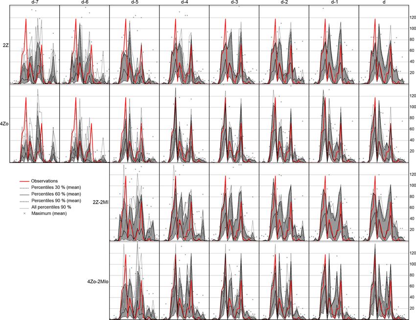
2918                                                                                                          P. Horton: AtmoSwing

Table 1. Reanalysis datasets that can be read by AtmoSwing.

         Name           Institution       Period of        Output          Model                       Model      Type of
                                          record           resolution      resolution                generation   input
         NR-1           NCEP, NCAR        1948–present     2.5◦ × 2.5◦     T62 (∼ 1.88◦ ), L28         1995       full
         NR-2           NCEP, DOE         1979–present     2.5◦ × 2.5◦     T62 (∼ 1.88◦ ), L28         2001       full
         ERA-INT        ECMWF             1979–present     0.75◦ × 0.75◦   TL255 (∼ 0.70◦ ), L60       2006       full
         20CR-2c        NOAA-CIRES        1851–2014        2◦ × 2◦         T62 (∼ 1.88◦ ), L28         2008       surface
         CFSR           NCEP              1979–present     0.5◦ × 0.5◦     T382 (∼ 0.31◦ ), L64        2009       full
         JRA-55         JMA               1958–present     1.25◦ × 1.25◦   TL319 (∼ 0.36◦ ), L60       2009       full
         JRA-55C        JMA               1958–2015        1.25◦ × 1.25◦   TL319 (∼ 0.36◦ ), L60       2009       conventional
         ERA-20C        ECMWF             1900–2010        1◦ × 1◦         TL159 (∼ 1.13◦ ), L91       2012       surface
         MERRA-2        NASA GMAO         1980–present     0.625◦ × 0.5◦   0.625◦ × 0.5◦ , L72         2014       full
         CERA-20C       ECMWF             1901–2010        1◦ × 1◦         T159 (∼ 1.13◦ ), L91        2016       surface
         ERA5           ECMWF             1979–present     0.25◦ × 0.25◦   TL639 (∼ 0.28◦ ), L137      2016       full

analogy on the levels 200, 500, and 850 hPa. Several pres-              dex (MI) based on the product of the relative humidity at
sure levels were later assessed by means of various crite-              850 hPa (RH850) and the total precipitable water (TPW) pro-
ria for the analogy based on the geopotential field (Duband,            vided the best skill (Table 2). Marty (2010) selected the MI at
1970, 1974, 1981; Guilbaud, 1997). It was found to be im-               925 hPa instead of 850 hPa and also considered the moisture
portant to calculate the analogy for multiple pressure levels           flux (MF) at 700 or 925 hPa (Table 2). The MF is the product
and different temporal windows (reference time of the pre-              of the MI with the wind intensity. Horton et al. (2018) de-
dictors as they are usually available at a 6-hourly temporal            termined that the MI values at 600 and 700 hPa were more
resolution or higher) instead of a unique selection (Guilbaud           useful than MF after the circulation analogy was applied
and Obled, 1998; Obled et al., 2002). Bontron (2004) showed             to the four atmospheric levels (Table 2). Ben Daoud et al.
that the choice of the temporal window can be more impor-               (2016) also reconsidered the parameters of the MI and ended
tant than the choice of the atmospheric level for daily precipi-        up with both 925 hPa and 700 hPa levels (Table 2). Subse-
tation (usually measured between 06:00 UTC and 06:00 UTC                quently, they added an additional level of analogy between
the following day). He concluded that the coupled geopoten-             the circulation and the moisture analogy (Table 2) based on
tial heights at 1000 hPa (Z1000) at 12:00 UTC and 500 hPa               the vertical velocity at 850 hPa (W850). This AM, termed
(Z500) at 24:00 UTC provided the best performance (for a                SANDHY for Stepwise Analogue Downscaling method for
subset of the NCEP/NCAR Reanalysis I – NR-1; Kalnay                     Hydrology (Ben Daoud et al., 2016; Caillouet et al., 2016),
et al., 1996; Kistler et al., 2001) for the investigated regions in     was primarily developed for large and relatively flat or low-
France (Table 2). The analogy of the atmospheric circulation            land catchments in France (Saône, Seine).
proposed by Bontron (2004) is still used operationally at the              Analogy criteria. In early applications of AMs, the geopo-
time of writing. Marty (2010) tested other temporal windows             tential height was condensed using principal component
for intraday application on the basis of a more comprehensive           analysis (PCA), and the selection of analog situations was
reanalysis dataset and proposed changing the hours of obser-            performed according to a Euclidean distance in the space
vation to 06:00 UTC and 18:00 UTC. Horton et al. (2018)                 of the PCA. Guilbaud (1997) stopped using PCA to work
showed that a selection of four combinations of pressure lev-           directly with the raw data interpolated on grids, which re-
els and temporal windows instead of two for the geopotential            sulted in an improvement. In the case of variables that de-
height improves the skill of the method (4Z, Table 2). The              scribe atmospheric circulation, the Teweles–Wobus (S1) cri-
pressure levels and temporal windows were automatically se-             terion (Eq. 1; Teweles and Wobus, 1954; Drosdowsky and
lected by genetic algorithms for the upper Rhône catchment              Zhang, 2003) was identified as the most suited criteria based
in Switzerland.                                                         on different studies (Wilson and Yacowar, 1980; Woodcock,
   Additional levels of analogy. Additional levels of analogy           1980; Guilbaud and Obled, 1998; Bontron, 2004). S1 allows
are subsequent steps that subsample a lower number of ana-              for a comparison of the gradients and thus an analogy of the
log situations from the antecedent level of analogy based on            atmospheric circulation instead of considering the actual val-
other variables. A second level of analogy was first intro-             ues at the grid points. For other predictors, classic criteria
duced by Mandon (1985) and Vallée (1986) based on wind,                 representing Euclidean distances between grid point values
moisture variables, or temperature. Gibergans-Báguena and               are used: mean absolute error (MAE) and root mean square
Llasat (2007) used the same kind of variables along with sta-
bility indexes. After a systematic assessment of the variables
provided by NR-1, Bontron (2004) noted that a moisture in-

Geosci. Model Dev., 12, 2915–2940, 2019                                                  www.geosci-model-dev.net/12/2915/2019/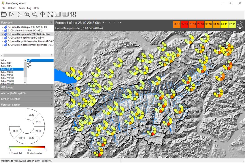
P. Horton: AtmoSwing                                                                                                                           2919

Table 2. Some existing analog methods listed by increasing complexity. P0 is the preselection (PC: on a calendar basis, which is ±60 d
around the target date), and L1, L2, and L3 are the subsequent levels of analogy. N1, N2, and N3 are the number of analogs to select at each
level of analogy. The meteorological variables are the following: Z – geopotential height, T – air temperature, W – vertical velocity, MI –
moisture index, which is the product of the relative humidity at the given pressure level and the total water column, and MF – moisture flux,
which is the product of MI with the wind intensity. The analogy criterion is S1 for Z and RMSE for the other variables.

  Type              P0                   L1                 N1    L2                       N2          L3          N3   Reference
  2Z                PC                   Z1000@12:00 UTC     50                                                         Bontron (2004)
                                         Z500@24:00 UTC
  4Z                PC                   Z1000@06:00 UTC   ∼ 27                                                         Horton et al. (2018)
                                         Z1000@30:00 UTC
                                         Z700@24:00 UTC
                                         Z500@12:00 UTC
  2Z-2MI            PC                   Z1000@12:00 UTC     70   MI850@12:00 UTC           30                          Bontron (2004)
                                         Z500@24:00 UTC           MI850@24:00 UTC
  2Z-2MI            PC                   Z1000@06:00 UTC     75   MI925@06:00 UTC           30                          Marty (2010)
                                         Z500@18:00 UTC           MI925@18:00 UTC
  2Z-2MF            PC                   Z1000@06:00 UTC     60   MF700@06:00 UTC∗          25                          Marty (2010)
                                         Z500@18:00 UTC           MF700@18:00 UTC
  4Z-2MI            PC                   Z1000@30:00 UTC   ∼ 63   MI700@24:00 UTC         ∼ 24                          Horton et al. (2018)
                                         Z850@12:00 UTC           MI600@12:00 UTC
                                         Z700@24:00 UTC
                                         Z400@12:00 UTC
  PT-2Z-4MI         T925@36:00 UTC       Z1000@12:00 UTC     70   MI925@12:00 UTC           25                          Ben Daoud et al. (2016)
                    T600@12:00 UTC       Z500@24:00 UTC           MI925@24:00 UTC
                                                                  MI700@12:00 UTC
                                                                  MI700@24:00 UTC
  PT-2Z-10MI        T925@36:00 UTC       Z1000@12:00 UTC     70   MI925@06:00–30:00 UTC     25                          Ben Daoud (2010)
                    T600@12:00 UTC       Z500@24:00 UTC           MI700@06:00–30:00 UTC
  PT-2Z-4W-4MI      T925@36:00 UTC       Z1000@12:00 UTC    170   W850@06:00 UTC            70   MI925@12:00 UTC   25   Ben Daoud et al. (2016)
                    T600@12:00 UTC       Z500@24:00 UTC           W850@12:00 UTC                 MI925@24:00 UTC
                                                                  W850@18:00 UTC                 MI700@12:00 UTC
                                                                  W850@24:00 UTC                 MI700@24:00 UTC

∗ or MF925@06:00 + 18:00 UTC as an alternative.

error (RMSE), the latter being used most often.                              of analogy. Using genetic algorithms, Horton et al. (2018)
            P                                                                introduced different spatial windows between the pressure
               |1ẑi − 1zi |                                                 levels, which increased the skill. Additionally, a weighting
             i
S1 = 100 P                     ,                                      (1)   between the predictors was also successfully added instead
           max |1ẑi |, |1zi |
              i
                                                                             of a simple equal-weights averaging. The number of analogs
                                                                             to select at each level of analogy should be optimized to be
where 1ẑi is the gradient between the ith pair of adjacent                  the best trade-off between taking into account local variabil-
points from the geopotential field of the forecasted target sit-             ity and maximizing useful synoptic information. It depends
uation, and 1zi is the corresponding observed geopotential                   on the predictor dataset, the size of the spatial window, and
gradient in the candidate situation. The differences are pro-                the length of the archive (Ruosteenoja, 1988; Van Den Dool,
cessed separately in both directions. The smaller the S1 val-                1994).
ues, the more similar the pressure fields. AtmoSwing allows                     Probabilistic forecast. After the last level of analogy, the
for the processing of real gradients by taking into account the              observed values of the predictand of interest (here daily pre-
actual distance between points or simple height differences                  cipitation amounts) for the Ni resulting dates provide the em-
by ignoring the horizontal distance. Under the latitudes of                  pirical conditional distribution considered to be the proba-
central Europe, the impact of neglecting the horizontal dis-                 bilistic forecast for the target day. The empirical frequencies
tance is small (not shown), but it can become more important                 are processed for every predictand value after classification
at higher latitudes.                                                         based on the Gringorten parameters (for a Gumbel or expo-
   Other parameters. The predictors are compared on a de-                    nential law; see Gringorten, 1963) and a probabilistic model
fined spatial window, which must be optimized to maximize                    can eventually be fitted (e.g., gamma function; Obled et al.,
the useful information and minimize noise. The spatial win-                  2002). The forecast is finally often synthesized according to
dow is usually considered unique for all predictors of a level

www.geosci-model-dev.net/12/2915/2019/                                                           Geosci. Model Dev., 12, 2915–2940, 2019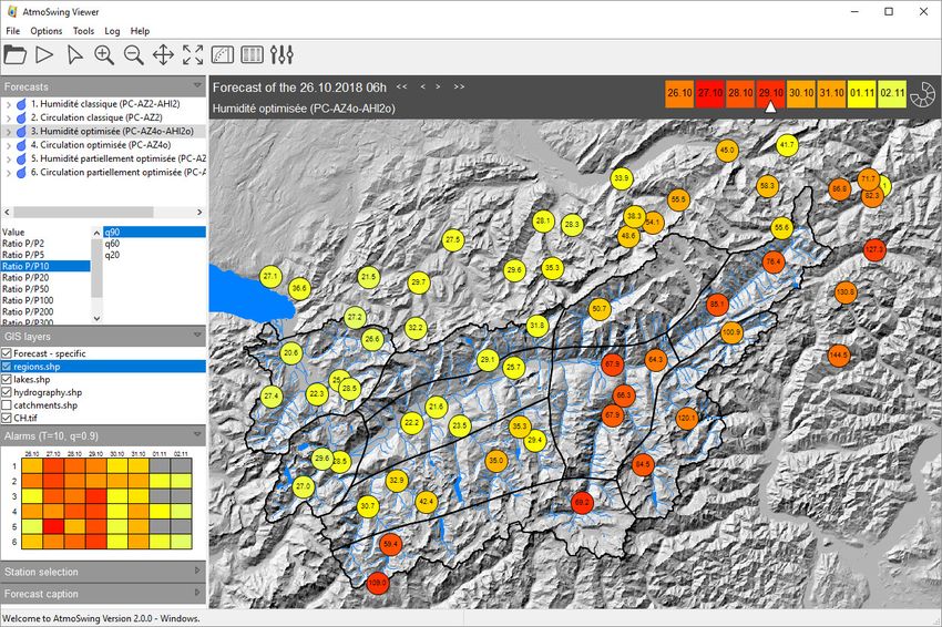
2920 P. Horton: AtmoSwing
percentiles 20 %, 60 %, and 90 % (Guilbaud, 1997; Guilbaud moSwing, a basic nomenclature is used (Fig. 2) in order to
and Obled, 1998). express the structure into a simple identifier. This cannot de-
Use in operational forecasting. In one of the very first uses scribe all the parameters of the AM, but it quickly illustrates
in operational forecasting, radiosonde observations were the structure of the method. This is particularly useful when
used as predictors to predict precipitation for the next 2 d. working with a global optimization method, wherein nothing
However, because of the chaotic nature of the atmosphere, is fixed but the structure of the AM. This nomenclature has
two analog situations quickly diverge over time (Lorenz, been used in Horton et al. (2017a, b, 2018) and Horton and
1969). Thus, the AM has strong limitations regarding the Brönnimann (2018).
analogy of temporal trajectories (Bontron, 2004). Given the The naming contains different blocs (separated by a hy-
superior capability of numerical models for simulating the phen) for the various levels of analogy. It starts with the spec-
dynamic evolution of the atmosphere, their outputs are now ification of the preselection (P; can be omitted when compar-
used as predictors for the coming days. The search for anal- ing AMs with the same preselection approaches), which can
ogy thus aims to connect the forecasted synoptic situation be one of two types.
with a local predictand, especially precipitation, which is
more difficult to simulate for numerical models. When using – PC: calendar period (±60 d around the target date)
AMs in operational forecasting, it should be noted that some
variables, such as moisture and vertical velocity, might not – PT: based on air temperature (Ben Daoud, 2010)
be accurately predicted after a lead time of a few days due to
Then, the following levels of analogy are listed, which
higher uncertainties. Predictors describing the atmospheric
may start with an optional A (for analogy). For every level
circulation are generally considered to be more reliable.
of analogy, the number of variables used (combination of at-
mospheric levels and time of observation) is first provided,
2.2.2 Regional characteristics
and then the short name of the variable is given (according
to, e.g., ECMWF conventions; in uppercase). Examples are
The optimal predictors vary from one region to another,
as follows.
along with the leading atmospheric processes. Thus, the
method needs to be adapted to local conditions, available – Z: geopotential (circulation)
data, and the size of the region of interest. Even for two loca-
tions that are close to each other but subject to different crit- – TPW: total precipitable water
ical atmospheric conditions, the selection of the best predic-
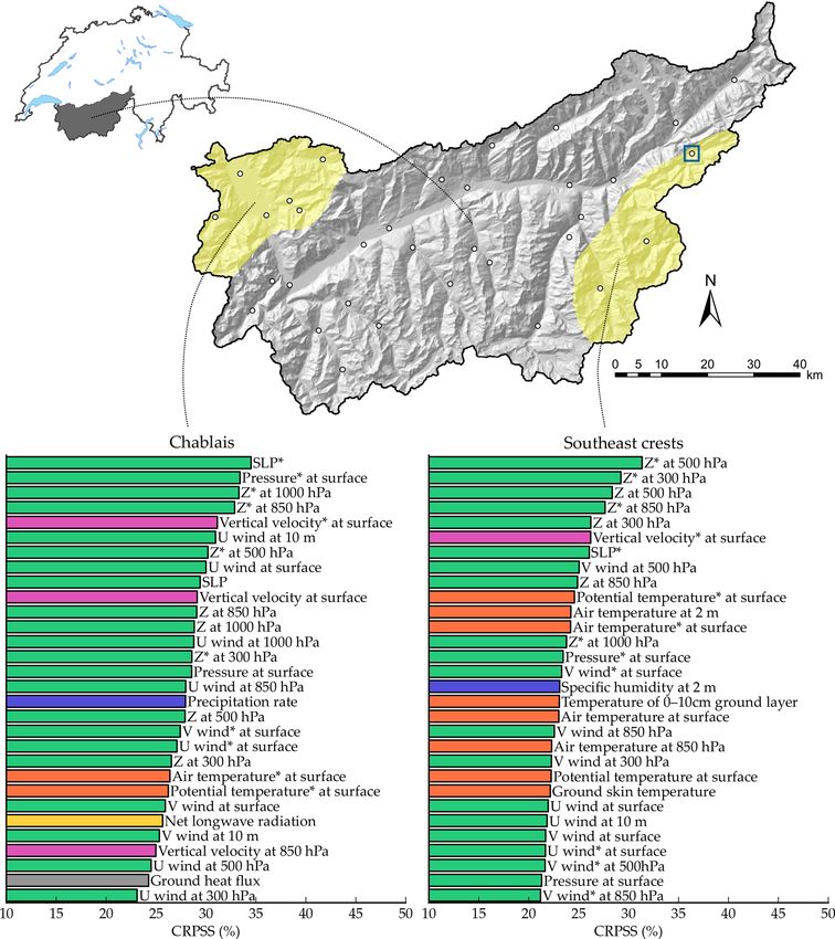
tors can vary. This is illustrated in Fig. 1 for two subregions – RH: relative humidity
of the Rhône catchment in Switzerland. For both subregions,
all variables of NR-1 were assessed by optimizing the spa- – V : wind velocity
tial window and the number of analogs for each one using
the sequential calibration tool implemented in AtmoSwing – W : vertical velocity
(Sect. 3.6.4). The main similarities in the selection of the best
predictor from NR-1 at both locations are that (1) the vari- – MI: moisture index (TPW · RH)
ables describing the atmospheric circulation (pressure fields
or geopotential heights) perform best, and (2) they are better – MF: moisture flux (V · TPW · RH)
when compared with the S1 criterion (asterisk in Fig. 1) in-
In order to keep the identifier simple, no value of atmo-
stead of the RMSE. The main difference is that the pressure
spheric level or time of observation is specified. Moreover,
fields better explain the precipitation when they are consid-
the analogy criterion is not specified and should be S1 for
ered close to the ground for the Chablais region, and at a
Z and RMSE for the other variables. If anything changes
higher altitude for the southeast crests. This is driven by the
from these conventions, it can be noted as a flag. The flag
elevation of the stations and by the main atmospheric drivers
(lowercase) can also provide other information, such as the
related to the precipitation at these locations.
optimization method.
The choice of the best predictors is likely to vary from one
reanalysis dataset to another. This comprehensive compari- – sc: sequential calibration (can be omitted as considered
son was not repeated with other datasets because a selection as default; see Sect. 3.6)
of the best predictors using genetic algorithms would be less
cumbersome (Sect. 3.6.5). – go (or just “o”): global optimization (by means of ge-
netic algorithms, for example)
2.2.3 Method nomenclature
This nomenclature can be adapted to specific needs or sim-
Variants of the AMs are numerous and it is not always easy plified for better readability (e.g., by removing the specifica-
to reference them in a short and descriptive way. In At- tion of the preselection). Examples can be found in Table 2.
Geosci. Model Dev., 12, 2915–2940, 2019 www.geosci-model-dev.net/12/2915/2019/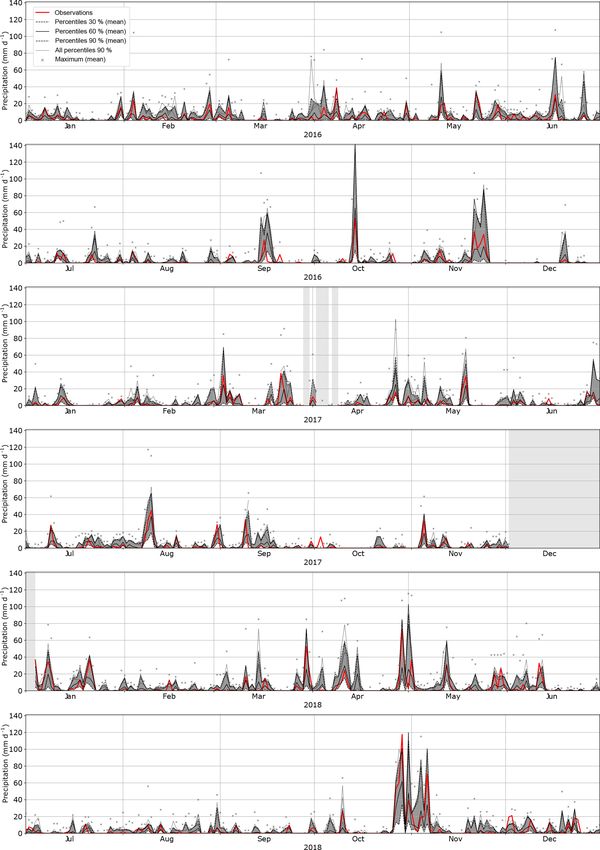
P. Horton: AtmoSwing                                                                                                                     2921

Figure 1. Performance score (CRPSS; Eq. 3; the reference being the climatological precipitation distribution) of the 30 best variables from the
NR-1 dataset, when considered separately (no combination), for the Chablais region and the southeast ridges in the upper Rhône catchment
in Switzerland. The analogy criterion is S1 when an asterisk is present next to the variable name and RMSE otherwise. Color illustrates
the variable type. Green: atmospheric circulation, blue: moisture, orange: temperature, yellow: radiation, purple: vertical velocity, and gray:
other. SLP stands for sea level pressure and Z for geopotential height. The blue square indicates the Binn station.

                                                                          tand. Separating the Forecaster and the Viewer allows for the
                                                                          automation of the forecast on a server and the local display
                                                                          of the results. The Forecaster, the Downscaler, and the Opti-
                                                                          mizer can be used either with a graphical user interface or a
                                                                          command-line interface.

                                                                          3.1   Technical aspects
Figure 2. Proposed nomenclature to describe the AM structure.
                                                                          The code is written in object-oriented C++ and relies on the
                                                                          wxWidgets (Smart et al., 2006) library to provide a cross-
3   AtmoSwing                                                             platform native experience to users. CMake is used to build
                                                                          AtmoSwing under Windows, Linux, or Mac OSX. Develop-
AtmoSwing is made up of four main modules that are stand-                 ments have been partly performed using a test-driven devel-
alone but do share a common code basis: the Forecaster for                opment (TDD) approach. Continuous integration has been
operational forecasting, the Viewer for displaying the fore-              set up (on Travis CI and AppVeyor) so that a collection of
cast in a GIS environment, the Downscaler for climate appli-              more than 600 tests can be evaluated on the three operat-
cations, and the Optimizer that is used to establish the statis-          ing systems every time new code is pushed to the server to
tical relationship that defines the analogy for a given predic-           prevent regressions. All analogy criteria, performance scores,

www.geosci-model-dev.net/12/2915/2019/                                                        Geosci. Model Dev., 12, 2915–2940, 2019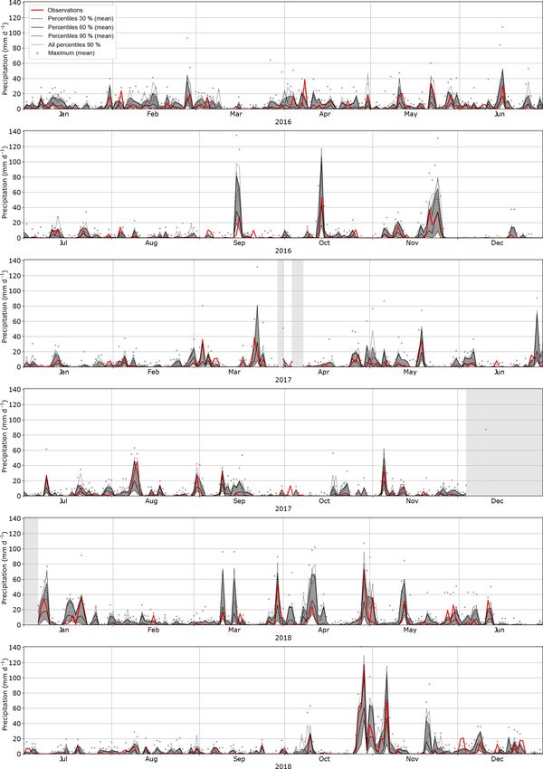
2922                                                                                                    P. Horton: AtmoSwing

searching and sorting functions, and data manipulations are
tested. Some tests specific to the AM rely on the results of
another analog sorting software developed at the Université
Grenoble Alpes. They ensure that the results of AtmoSwing
are exactly equivalent to this model given the same parame-
ters and data. The source code is under version control (Git)
and is open source (on GitHub; Horton, 2018a). The GitHub
organization page also contains toolboxes to work with the
outputs of AtmoSwing in R (Horton and Burkart, 2018) or
Python (Horton, 2018b).
   Although processing an analog adaptation for a given tar-
get date is fast, numerous hindcasts over periods of sev-
eral decades must be performed for calibration, which may
become very time-consuming. Thus, great effort has been
focused on minimizing the processing time using profiling
tools. Firstly, all identified redundancies in the processing
were removed. Then, when searching for a certain date or
data, the search starts in the region where it is likely to be
found instead of exploring an entire array. Similar data are
                                                                   Figure 3. Simplified flowchart of the AM implementation in At-
not loaded twice, but instead shared pointers are used. Sev-       moSwing.
eral other improvements allow for a reduction in computing
time, for example the use of the “quicksort” method (Hoare,
1962) to sort the date vectors according to the analogy cri-
terion. Different implementation variants were tested in or-       the predictand (at the final stage), and other data. This object
der to select the most efficient approach: for example, when       can be saved as a NetCDF file and/or can be injected into a
storing analog dates according to their criterion value, it is     new analogy level. The whole structure of the AM is defined
faster to insert them in a fixed-size array instead of storing     through an XML file. Even the time step of the method (6 or
them all and subsequently sorting the array. When using the        24 h, for example) is a dynamic parameter.
S1 criterion, the gradients are preprocessed on the predictor         Each implementation of the AM (see Sect. 2.2) may en-
data so that they are only processed once. AtmoSwing also          ter this scheme, even if it consists of preprocessed variables
uses the linear algebra library Eigen 3 (Guennebaud et al.,        (e.g., moisture index). Various preprocessing functions are
2010) for calculations on vectors and matrices, which results      implemented as the calculation of the moisture index or flux,
in time-saving. Multi-threading is also implemented so that        multiplication operations, or calculation of the gradients. The
the search for analog situations in the archive is distributed     user can dynamically specify the preprocessing method and
among the available threads.                                       the predictors to use in the XML file.
   A user interface allows for the creation of the predictand         This modular approach is implemented through object-
database in NetCDF format from text files. During the pro-         oriented programming as a direct consequence of polymor-
cess, Gumbel adjustments are automatically calculated for          phism. This allows, for example, for the processing of a pre-
precipitation data to determine the values corresponding to        dictor object as a single interface to entities representing any
different return periods. The time series are normalized using     reanalysis dataset. Similarly, the criterion can be of different
a selected return period (default 10 years) and their square       types, as can the score for calibrating. The different types of
root can be processed. The final database file contains both       objects that are instantiated are defined in the XML parame-
the raw and the normalized series, as well as characteristics      ter file. Thus, there is a single implementation of the analog
of the gauging stations and some metadata.                         method capable of interacting with different types of objects
                                                                   in various contexts (calibration, forecasting, downscaling).
3.2    Modular approach and implementation
                                                                   3.3   AtmoSwing Forecaster
AtmoSwing’s great strength is that it is designed to process
the analog method in a modular fashion. The structure of           The Forecaster module allows for the processing of opera-
the AM (number of analogy levels, number of predictors)            tional forecasts. The software can be compiled with a graph-
is built dynamically (Fig. 3), and nothing is fixed a priori.      ical user interface (GUI), or without it, to be used on a head-
The software then successively performs as many analogy            less server through a command-line interface (CLI). Process-
levels as the user specifies using all the predictors indicated.   ing a forecast requires very low computing capabilities and
Each level of analogy results in an object containing target       can be performed on a low-end computer. It successfully runs
dates, analog dates, values of the analogy criteria, values of     on a Raspberry Pi 3 (Model B).

Geosci. Model Dev., 12, 2915–2940, 2019                                              www.geosci-model-dev.net/12/2915/2019/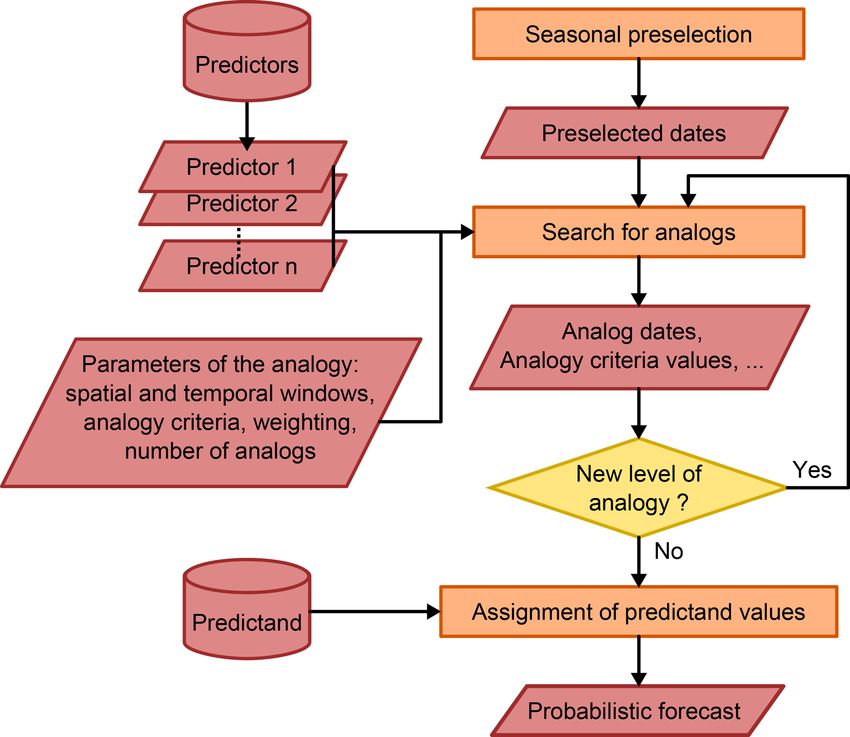
P. Horton: AtmoSwing                                                                                                           2923

   To this day, the software can use the outputs of IFS or GFS      (which can be changed in the preferences). This highest level
(see Sect. 2.1). When possible, it first downloads the relevant     of synthesis allows for quick identification of potentially crit-
model outputs and interpolates the gridded data to match the        ical situations in the days ahead.
resolution of the archive. The analog dates are next extracted         Then, the user can explore the forecasts in more detail,
according to the selected AM variant and the predictand data        starting from the provided map (Fig. 4). The map displays
are associated with the corresponding dates. The results are        the forecast of the selected AM variant (selected in the up-
finally saved in auto-describing NetCDF files. If requested,        per left panel) and the selected lead time (upper right). Dur-
a synthetic XML file is generated for easier integration on a       ing the forecast, one AM might have parameters that differ
web platform, for example. Every step of the forecast, from         by subregion, such as the number of analogs or the spatial
predictor downloading (when possible) to the final results, is      windows. The Viewer automatically gathers the similar AM
performed in the software (and controlled through configu-          types and provides a composite view of the optimal forecasts
ration) without the use of external scripts (e.g., for data con-    per subregion. The user can, however, choose to display the
version).                                                           results associated with a single parameter set for the entire
   Both the GUI and the CLI facilitate the processing of a          region (by opening the tree view and selecting a child ele-
forecast based on the most recent NWP outputs or for a given        ment), which provides a homogeneous set of analog dates. A
date or period. When there are no new predictor data avail-         display of all lead times on a single map is possible based on
able, the forecast is not processed and computing resources         a symbolic representation on a circular band with a box for
are not consumed. The recommended use is thus to set up             every lead time (Fig. 5). The number of boxes is adjusted to
an automatic task on a server to trigger the forecast every         the number of lead times. This representation offers a global
30 min. This would, for example, provide four forecasts a           spatiotemporal visualization for a chosen AM.
day.                                                                   Color scales in the map can be adjusted by choosing (on
   Before being used in operational forecasting, the AMs            the left part of the GUI) the predictand reference (raw value
were calibrated in a perfect prognosis framework, usually us-       or ratio to different return periods) and the quantile of the
ing a reanalysis dataset (Sect. 3.6). However, this does not        distribution. Using a ratio to a certain return period eases the
take into account the uncertainty related to the forecast of        interpretation of the expected precipitation given that refer-
the target situation by NWP models. One might be willing to         ence values can drastically differ from one location to an-
take into account this uncertainty, which increases with the        other, particularly in mountainous regions. All information
lead time. A solution is to increase the number of analog sit-      relative to a rain gauge station (or catchment), such as its lo-
uations with the lead time, which should be optimized for           cation, its name, and the values of different return periods, is
every lead time on a forecast archive or a reforecast dataset       stored in the forecast files to be displayed for end users who
(Thevenot, 2004). This technique is available in AtmoSwing,         do not have the predictand database.
as the number of analogs can be specified for every lead time.         By clicking on a station on the map (or by selection from
   A meteorological variable that proved to be a good pre-          a dropdown list on the left), a new window appears with a
dictor in the perfect prognosis framework may eventually be         plot of the forecasted time series (Fig. 6). By default, the plot
poorly predicted by the selected NWP beyond a certain lead          contains the usual three considered percentiles (9th, 60th,
time. It should then be dropped after this lead time. For ex-       and 20th), along with the 10 best analogs (crosses) with a
ample, when using moisture variables for the second level           color code from yellow (10th) to red (first). The 10-year re-
of analogy, Thevenot (2004) showed that beyond a lead time          turn period value is also displayed as a red line. The user can
of 3 d the AM with two levels did not perform better than           choose to hide any data or to display supplementary informa-
the one with a single level of analogy. Datasets of reforecasts     tion (all analogs, all 10th percentiles, or all return periods)
from the selected NWP models allow for the assessment of            in the left panel. Traces of previous forecasts are also auto-
these aspects for different lead times.                             matically loaded and displayed to provide information on the
                                                                    consistency of the forecasts.
3.4   AtmoSwing Viewer                                                 The user can then delve into further detail and display
                                                                    the predictand cumulative distribution for a given lead time
The AtmoSwing Viewer allows for the display of the files            (Fig. 7). This can help determine whether there is a shift be-
produced by the Forecaster in an interactive GIS environ-           tween the distribution of all analogs versus the 10 best. Such
ment (Fig. 4) with several levels of synthesis. It first provides   a shift warns of a risk of underestimation and/or overestima-
an overview of possible alerts using color codes on the lead        tion when considering the full distribution, particularly for
time switcher (upper right in the GUI; see Fig. 4), which rep-      high precipitation amounts. Indeed, the number of extreme
resent the worst-case scenarios, or in the alarm panel (on the      precipitation events in the archive is limited and they are thus
left side of the GUI). The alarm panel allows for a synthe-         likely to be under-represented in the selected analog dates.
sis of the highest forecasted values for the different AMs and      Different authors have shown that if the 60th percentile is
the different lead times. By default, the colors are expressed      best to forecast the occurrence and the amount of precipi-
relative to the 10-year return period for the 90th percentile       tation for common situations, the 90th percentile is a bet-

www.geosci-model-dev.net/12/2915/2019/                                                Geosci. Model Dev., 12, 2915–2940, 2019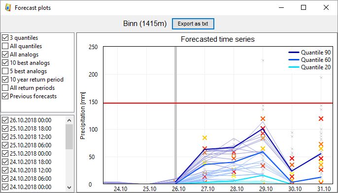
2924                                                                                                             P. Horton: AtmoSwing

Figure 4. Graphical user interface of the Viewer module (elevation data from the Shuttle Radar Topography Mission – SRTM; hydrological
network from SwissTopo). The values on the map represent the 90th percentile (as selected on the left panel) of the precipitation values from
the analog samples at the different stations and for the selected lead time. The color is proportional to the selected return period (10 years
here).

ter indicator for strong to extreme events (Djerboua, 2001;              3.5    AtmoSwing Downscaler
Bontron, 2004; Marty, 2010). It is therefore necessary to pay
close attention when the 90th percentile reaches high values,            The Downscaler module is the last addition to AtmoSwing.
as this may be indicative of possible extreme precipitation              Its purpose is to downscale either climate model outputs for
due to the presence of several analog dates with high precip-            climate impact studies or reanalyses for climate reconstruc-
itation amounts in the distribution (Djerboua, 2001).                    tion of the past.
   The distribution of the analogy criteria (not shown) can                 The Downscaler is able to read outputs of general circu-
also be displayed to identify eventual discontinuities in the            lation models (GCMs) or regional climate models (RCMs),
criteria values. Finally, one can display the analog dates with          such as the Coupled Model Intercomparison Project Phase
the corresponding predictand criteria values in an interactive           5 (CMIP5; Taylor et al., 2012) and EURO-CORDEX (Jacob
spreadsheet (not shown).                                                 et al., 2014), and can be extended to other datasets. CMIP5
   The AtmoSwing Viewer relies on workspace files provid-                and EURO-CORDEX are distributed in the NetCDF format
ing the path to the forecast directories and the GIS layers. It          but present a great variety of time steps, temporal references,
is thus easy to switch from a forecast for a region to another.          spatial resolution, and file structures. A complete redesign
Many GIS formats are supported thanks to GDAL (Geospa-                   of the management of the predictor data was necessary to
tial Data Abstraction Library; GDAL Development Team,                    provide the flexibility required to account for this variety.
2014). A user can have as many layers as desired and can                 The Downscaler is thus able to parse the original files in
control their display properties (color, transparency).                  these datasets by exploiting the self-descriptive capacity of
                                                                         NetCDF files.

Geosci. Model Dev., 12, 2915–2940, 2019                                                      www.geosci-model-dev.net/12/2915/2019/
P. Horton: AtmoSwing 2925 Figure 5. Same as Fig. 4 but for multiple lead times. Figure 6. Visualization of the forecasted time series for an event at the Binn station (Fig. 1) in October 2018. The thick blue lines represent the 90th, 60th, and 20th percentiles for the given lead times. The thin blue lines represent the equivalent time series but from previous forecasts. The small gray crosses represent all analog values and the larger crosses highlight the 10 best analogs (with a color gradient from red for the best to yellow for the 10th). www.geosci-model-dev.net/12/2915/2019/ Geosci. Model Dev., 12, 2915–2940, 2019
2926                                                                                                                 P. Horton: AtmoSwing

Figure 7. Visualization of the forecasted precipitation distribution for a given lead time for an event at the Binn station (Fig. 1) in October
2018. The blue line represents the full distribution provided by all analogs, the circles are the 90th, 60th, and 20th percentiles, and the crosses
correspond to the distribution provided by the 10 best analogs (with a color gradient from red for the best to yellow for the 10th). The vertical
red line here is the precipitation value for a 10-year return period.

    The use of AMs in the context of future climate is rather               establishes the relationship based on model outputs. As a re-
new. Not all AMs can be used for this purpose because some                  sult, perfect prognosis yields relationships that are as close as
predictors might not capture the climate change signal well,                possible to the natural links between predictors and predic-
and the preservation of the relationship between predictors                 tands. However, there are no perfect models and even reanal-
and predictands must prevail. However, several authors have                 ysis data may contain biases that cannot be ignored (Dayon
demonstrated the transferability of some AMs for future cli-                et al., 2015; Horton and Brönnimann, 2018). Thus, the con-
mate (Dayon et al., 2015, 2018; Raynaud, 2016; Turco et al.,                sidered predictors should be as robust as possible; i.e., they
2017). The transferability of an AM must be assessed before                 should have minimal dependency on the model. With MOS
it is used in such a context.                                               approaches, reforecasts can be used to establish the relation-
    AMs have also been used to perform climate reconstruc-                  ship between predictors and predictands, provided that the
tion of the past (Caillouet et al., 2016, 2017; Bonnet et al.,              archive is long enough. However, the calibration procedure
2017). Such applications allow, for example, for the hydro-                 must be performed every time a new version is available in
logical modeling of flood events in periods during which no                 order to reduce the bias (Wilson and Vallée, 2002).
meteorological data are available or analysis of past severe                   A statistical relationship is established with a trial-and-
droughts.                                                                   error approach by processing a forecast for every day of a
                                                                            calibration period. A certain number of days close to the
3.6     AtmoSwing Optimizer                                                 target date is excluded to consider only independent can-
                                                                            didate days. Validating the parameters of AMs on an inde-
The AtmoSwing Optimizer is a single tool that integrates dif-               pendent validation period is very important to avoid over-
ferent optimization methods, presented in Sect. 3.6.3 to 3.6.5.             parametrization and to ensure that the statistical relation-
Its purpose is to establish the statistical relationship between            ship is valid for another period. In order to account for cli-
the predictors and a predictand. The calibration framework                  mate change and the evolution of measuring techniques, it is
is detailed in Sect. 3.6.1 and the implemented skill scores are             recommended that a noncontinuous period for validation be
listed in Sect. 3.6.2.                                                      used, distributed over the entire archive (Ben Daoud, 2010;
                                                                            Horton and Brönnimann, 2018). AtmoSwing’s users can thus
3.6.1    Calibration framework                                              specify a list of the years to set apart for the validation that
                                                                            are removed from possible candidate situations. At the end of
The calibration of the AM is usually performed in a perfect                 the optimization, the validation score is processed automati-
prognosis (Klein et al., 1959) framework (Bontron, 2004;                    cally.
Ben Daoud, 2010). Perfect prognosis uses observed or re-
analyzed data to calibrate the relationship between predic-
tors and predictands, as opposed to the MOS approach that

Geosci. Model Dev., 12, 2915–2940, 2019                                                         www.geosci-model-dev.net/12/2915/2019/
P. Horton: AtmoSwing 2927
3.6.2 Implemented performance scores Continuous probabilistic predictions. These types of pre-
dictions are issued in the form of the expected statistical dis-
Multiple scores are implemented in the AtmoSwing Op- tribution for a variable, which needs to be compared to an
timizer and are listed hereafter. Details are only provided observed value. This is the situation encountered when using
for the CRPS (continuous ranked probability score; Brown, multiple analogs from AMs.
1974; Matheson and Winkler, 1976; Hersbach, 2000), which Most assessments of AM performance use the CRPS (con-
is most often used. tinuous ranked probability score; Brown, 1974; Matheson
Discrete deterministic predictions. These are, for example, and Winkler, 1976; Hersbach, 2000). It allows for evaluation
deterministic predictions of threshold exceedances. The con- of the predicted cumulative distribution functions F (y), for
tinuous probabilistic nature of an ensemble of analogs can example the precipitation values y associated with the analog
be transformed into a discrete prediction by considering a situations compared to the single observed value y 0 for a day
fixed percentile from the distribution, which is compared to i:
a threshold exceedance of the predictand. On the basis of a
contingency table (Wilks, 2006), multiple scores can be pro- Z+∞h i2
cessed with AtmoSwing. These include the following. CRPSi = Fi (y) − H (y − yi0 ) dy, (2)
0
– Proportion correct (Finley, 1884)
where H (y − yi0 ) is the Heaviside function that is null when
– Threat score (Gilbert, 1884) y − yi0 < 0 and has the value 1 otherwise; the better the pre-
diction, the lower the score. This score is now commonly
– Bias
used for the evaluation of continuous variable prediction sys-
– False alarm ratio tems (Casati et al., 2008; Marty, 2010). It can be decom-
posed into several indicators also implemented into the At-
– Hit rate or probability of detection moSwing Optimizer, such as reliability and resolution (Hers-
bach, 2000) or sharpness and accuracy (Bontron, 2004).
– False alarm rate Its skill score expression is often used, with the clima-
tological distribution of precipitation as the reference. The
– Heidke skill score (Heidke, 1926) CRPSS (continuous ranked probability skill score) is thus de-
fined as follows (Bradley and Schwartz, 2011):
– Peirce skill score (Peirce, 1884)
CRPS
– Gilbert skill score or equitable threat score (Gilbert, CRPSS = 1 − , (3)
CRPSclim
1884)
where CRPSclim is the CRPS value for the climatological dis-
Continuous deterministic predictions. These types of pre-
tribution. A better prediction is characterized by an increase
dictions must be evaluated using distance measures. For
in CRPSS.
AMs, the provided distribution is summarized by a chosen
Finally, the rank diagram (Talagrand et al., 1997) and its
percentile, which is compared to the predictand value. Avail-
accuracy as defined by Candille and Talagrand (2005) are
able scores are as follows.
also available.
– Mean absolute error
3.6.3 The sequential calibration
– Root mean square error
The calibration procedure that we call “sequential” or “clas-
Discrete probabilistic predictions. Here, the probability of sic” was elaborated upon by Bontron (2004) (see also
occurrence or the probability of belonging to a certain cate- Radanovics et al., 2013; Ben Daoud et al., 2016). It is a semi-
gory is considered. The implemented scores are as follows. automatic procedure that optimizes the spatial windows in
which the predictors are compared and the number of analogs
– Brier score (Brier, 1950) for every level of analogy. The different analogy levels (e.g.,
the atmospheric circulation or moisture index) are calibrated
– ROC diagram (relative operating characteristic or re- sequentially. The procedure consists of the following steps
ceiver operating characteristic; Mason, 1982) (Bontron, 2004).
– RPS (ranked probability score; Epstein, 1969) 1. Manual selection of the following parameters:
– SEEPS (stable equitable error in probability space; Rod- (a) meteorological variable,
well et al., 2010, 2011) (b) pressure level,
www.geosci-model-dev.net/12/2915/2019/ Geosci. Model Dev., 12, 2915–2940, 20192928 P. Horton: AtmoSwing
(c) temporal window (hour of the day), and 3.6.4 Variable exploration
(d) number of analogs.
The sequential calibration can also be used to explore the
2. For every level of analogy, the following steps are taken. variables of a dataset. A list of variables, pressure levels, and
temporal windows can be provided and all combinations are
(a) The most skilled unitary cell is identified (four assessed through the classic(+) calibration. This functional-
points for the geopotential height when using the ity facilitates a comparison between the different variables
S1 criterion and one point otherwise) of the predic- of a dataset while considering the effect of the pressure level
tor data over a large domain. Every point or cell of and the temporal window. Using this approach, only one vari-
the full domain is assessed based on the predictors able is assessed at a time, but multiple levels of analogy are
of the current level of analogy. possible. Figure 1 results from such an analysis of the NR-1
reanalysis.
(b) From this most skilled cell, the spatial window is
expanded by successive iterations in the direction 3.6.5 Global optimization
of the largest performance gain until no further im-
provement is possible. The sequential calibration has strong limitations: (i) it can-
(c) The number of analog situations Ni , which was ini- not automatically choose the pressure levels and temporal
tially set to an arbitrary value, is then reconsidered windows (hour of the day) for a given meteorological vari-
and optimized for the current level of analogy. able, (ii) it cannot handle dependencies between parameters,
and (iii) it cannot easily handle new degrees of freedom. For
3. A new level of analogy can then be added based on other this reason, genetic algorithms (GAs) were implemented in
variables such as the moisture index at chosen pressure the AtmoSwing Optimizer to perform a global optimization
levels and hours of the day. The procedure starts again of AMs. This allows for the optimization of all parameters
from step 2 (calibration of the spatial window and the jointly in a fully automatic and objective way. The method
number of analogs) for the new level. The parameters is described in Horton et al. (2017a) and an application is
calibrated for the previous analogy levels are fixed and provided in Horton et al. (2018).
do not change.
3.6.6 Monte Carlo simulations
4. Finally, the numbers of analogs for the different levels
of analogy are reassessed. This is performed iteratively A Monte Carlo analysis is also implemented in AtmoSwing.
by varying the number of analogs of each level in a sys- The procedure performs thousands of assessments of random
tematic manner. parameters within given ranges. This method is not efficient
for finding the best parameter set, but it facilitates a better un-
The calibration is performed in successive steps for a lim- derstanding of the sensitivity of the parameters. Its relevance
ited number of parameters with the aim of minimizing error is, however, limited for AMs with multiple levels of anal-
functions or maximizing skill scores. Except for the num- ogy and variables. Indeed, for methods with a high number
ber of analogs, previously calibrated parameters are gener- of parameters with wide authorized value ranges, the prob-
ally not reassessed. The benefit of this method is that it is ability is too low to obtain an acceptable configuration, and
relatively fast, it provides acceptable results, and it has low thus the resulting response surface might not be representa-
computing requirements. tive of the actual distribution of optimal values (see examples
Small improvements were incorporated into this method in Sect. 4).
in the AtmoSwing Optimizer, then termed as “classic+”, by
allowing the spatial windows to perform other moves, such
as (1) an increase in two simultaneous directions, (2) a de- 4 Parameter space of AMs
crease in one or two simultaneous directions, (3) expansion
or contraction (in every direction), (4) a shift of the window An analysis of the parameters resulting from Monte Carlo
(without resizing) in eight directions (including diagonals), simulations, the sequential calibration, and GAs was per-
and finally (5) all the moves described above, but with a fac- formed for the Binn station in Switzerland (Fig. 1) with
tor of 2, 3, or more. For example, an increase by two grid ERA-INT (Table 1). High precipitation in the Binn region
points in one (or more) direction is assessed. This allows one was responsible for large damage downstream on several oc-
size, which may not be optimal, to be skipped. These supple- casions, making it a station of particular interest. The results
mentary steps often result in spatial windows that are slightly for this station cannot be generalized to all stations, but sim-
different. The performance gain is rather marginal for reanal- ilar conclusions can be drawn for other locations. Moreover,
yses with a low resolution such as NR-1, but might be more the parameter space at a single station is expected to be less
consistent for reanalyses with higher resolutions due to the regular than averaged regional precipitation. For all analyses,
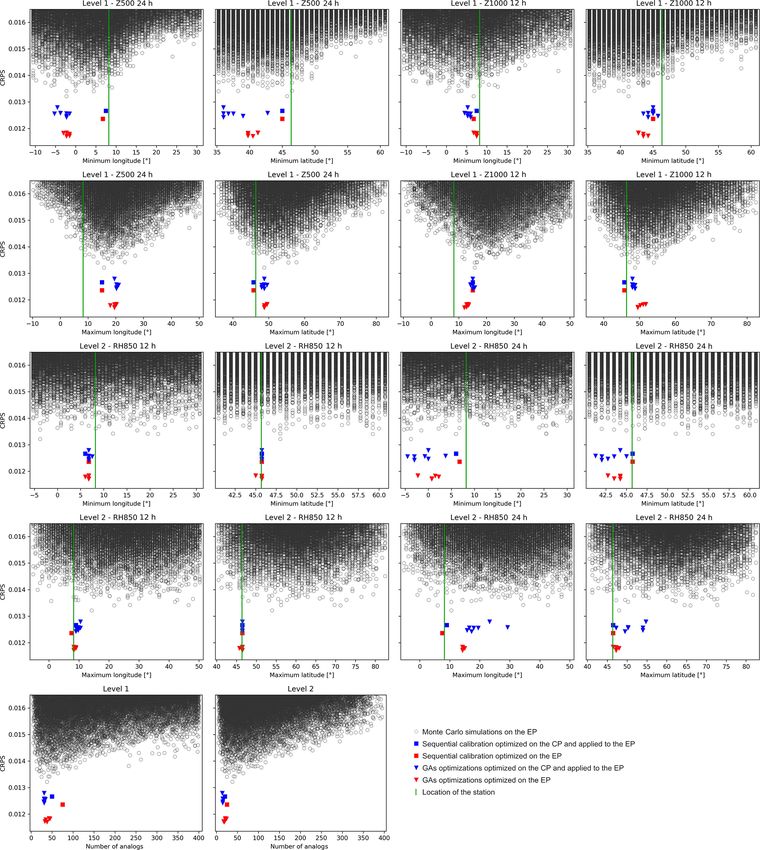
presence of more local minima. the archive period is 1981–2010 and the results are shown for
Geosci. Model Dev., 12, 2915–2940, 2019 www.geosci-model-dev.net/12/2915/2019/You can also read