Simulating the atmospheric CO2 concentration across the heterogeneous landscape of Denmark using a coupled atmosphere-biosphere mesoscale model ...
←
→
Page content transcription
If your browser does not render page correctly, please read the page content below
Biogeosciences, 16, 1505–1524, 2019
https://doi.org/10.5194/bg-16-1505-2019
© Author(s) 2019. This work is distributed under
the Creative Commons Attribution 4.0 License.

Simulating the atmospheric CO2 concentration across the
heterogeneous landscape of Denmark using a coupled
atmosphere–biosphere mesoscale model system
Anne Sofie Lansø1,a , Thomas Luke Smallman2,3 , Jesper Heile Christensen1,4 , Mathew Williams2,3 , Kim Pilegaard5 ,
Lise-Lotte Sørensen4 , and Camilla Geels1
1 Department  of Environmental Science, Aarhus University, Frederiksborgvej 399, 4000 Roskilde, Denmark
2 School of GeoSciences, University of Edinburgh, Edinburgh, EH9 3JN, UK
3 National Centre for Earth Observation, University of Edinburgh, Edinburgh, EH9 3JN, UK
4 Arctic Research Centre (ARC), Department of Bioscience, Aarhus University, Ny Munkegade 114, 8000 Aarhus, Denmark
5 Department of Environmental Engineering, Technical University of Denmark (DTU), Bygningstorvet 115,

2800 Kongens Lyngby, Denmark
a now at: Laboratoire des Sciences du Climat et l’Environnement, LSCE/IPSL, CEA-CNRS-UVSQ,

Université Paris-Saclay, 91191 Gif-sur-Yvette, France

Correspondence: Anne Sofie Lansø (anne-sofie.lanso@lsce.ipsl.fr)

Received: 23 May 2018 – Discussion started: 27 June 2018
Revised: 22 February 2019 – Accepted: 15 March 2019 – Published: 10 April 2019

Abstract. Although coastal regions only amount to 7 % of            tower is positioned next to Roskilde Fjord, the local marine
the global oceans, their contribution to the global oceanic         impact was not distinguishable in the simulated concentra-
air–sea CO2 exchange is proportionally larger, with fluxes in       tions. But the regional impact from the Danish inner waters
some estuaries being similar in magnitude to terrestrial sur-       and the Baltic Sea increased the atmospheric concentration
face fluxes of CO2 .                                                by up to 0.5 ppm during the winter months.
   Across a heterogeneous surface consisting of a coastal
marginal sea with estuarine properties and varied land mo-
saics, the surface fluxes of CO2 from both marine areas and
terrestrial surfaces were investigated in this study together       1   Introduction
with their impact in atmospheric CO2 concentrations by the
usage of a high-resolution modelling framework. The simu-           Understanding the natural processes responsible for absorb-
lated terrestrial fluxes across the study region of Denmark ex-     ing just over half of the anthropogenic carbon emitted to
perienced an east–west gradient corresponding to the distri-        the atmosphere will help decipher future climatic pathways.
bution of the land cover classification, their biological activ-    During the last decade, the ocean and the biosphere are esti-
ity and the urbanised areas. Annually, the Danish terrestrial       mated to take up to 2.4 ± 0.5 and 3.0 ± 0.8 PgC yr−1 of the
surface had an uptake of approximately −7000 GgC yr−1 .             9.4±0.5 PgC yr−1 of anthropogenic carbon emitted to the at-
While the marine fluxes from the North Sea and the Dan-             mosphere (Le Quéré et al., 2018). The heterogeneity and the
ish inner waters were smaller annually, with about −1800            dynamics of the surface complicates such estimates.
and 1300 GgC yr−1 , their sizes are comparable to annual ter-          Biosphere models of various complexity have been de-
restrial fluxes from individual land cover classifications in       veloped to spatially simulate surface fluxes of CO2 , but
the study region and hence are not negligible. The contribu-        future estimates of the land uptake are bound with large
tion of terrestrial surfaces fluxes was easily detectable in both   uncertainties (Friedlingstein et al., 2014) that can be at-
simulated and measured concentrations of atmospheric CO2            tributed to model structural uncertainties, uncertain obser-
at the only tall tower site in the study region. Although, the      vations and lack of model benchmarking (Cox et al., 2013;

Published by Copernicus Publications on behalf of the European Geosciences Union.
1506                                                A. S. Lansø et al.: CO2 across the heterogeneous landscape of Denmark

Luo et al., 2012; Lovenduski and Bonan, 2017). To have the         Mørk et al., 2016) are not always included in marine mod-
best chance of accurately predicting the future evolution of       els (Omstedt et al., 2009; Gypens et al., 2011; Kuznetsov and
the carbon cycle, and its implications for our climate, it is      Neumann, 2013; Gustafsson et al., 2015; Valsala and Mur-
important to minimise the uncertainties that exist presently       tugudde, 2015), let alone being taken into account in at-
(Carslaw et al., 2018). Enhanced knowledge and a better pro-       mospheric mesoscale systems simulating CO2 (Sarrat et al.,
cess understanding in ecological theory and modelling could        2007a; Geels et al., 2007; Law et al., 2008; Tolk et al., 2009;
potentially reduce the model structural uncertainties (Loven-      Broquet et al., 2011; Kretschmer et al., 2014). But a recent
duski and Bonan, 2017), which together with improvements           study found that short-term variability in the partial pressure
in spatial surface representation could minimise the current       of surface water CO2 (pCO2 ) can substantially affect sim-
uncertainties.                                                     ulated annual fluxes in certain coastal areas – in their case
   Studying surface exchanges of CO2 on regional to lo-            the Baltic Sea (Lansø et al., 2017). Moreover, direct eddy co-
cal scale can be accomplished with mesoscale atmospheric           variance (EC) measurements in the Baltic Sea have shown
transport models. Their resolution is in the range from 2 to       that upwelling events with rapid changes in pCO2 greatly
20 km, and their advantage is their capability to get a better     increase the air–sea CO2 exchange (Kuss et al., 2006; Rut-
process understanding of both atmospheric and surface ex-          gersson et al., 2009; Norman et al., 2013).
change mechanisms in order to improve the link between ob-            In this study we aim to simulate surface exchanges of
servations and models at all scales, i.e. for both mesoscale,      CO2 at a high spatio-temporal resolution across a region
regional and global models (Ahmadov et al., 2007). The             neighbouring the Baltic Sea, alternating between land and
higher spatial resolution of mesoscale models allows for a         coastal sea together with mesoscale atmospheric transport.
better representation of atmospheric flows and for a more de-      A newly developed mesoscale modelling system is used
tailed surface description, which is necessary in particular       to assess and understand the dynamics and relative impor-
for heterogeneous areas. In previous mesoscale model stud-         tance of the marine and terrestrial CO2 fluxes. The Danish
ies, biosphere models have been coupled to the mesoscale           Eulerian Hemispheric Model (DEHM) forms the basis of
atmospheric models ranging in their complexity, from a sim-        the framework, while the mechanistic biospheric soil–plant–
ple diagnostic (Sarrat et al., 2007b; Ahmadov et al., 2007,        atmosphere model (SPA) is dynamically coupled to the at-
2009) to mechanistic-process-based biosphere models (Tolk          mospheric model. Both models are driven by methodologi-
et al., 2009; Ter Maat et al., 2010; Smallman et al., 2014;        cal data from the Weather Research and Forecasting model
Uebel et al., 2017). The modelled CO2 concentrations and           (WRF). The air–sea CO2 exchange is simulated at a high
surface fluxes from mesoscale model systems compare bet-           temporal resolution with the best applicable surface fields
ter with observations than global model systems (Ahmadov           of pCO2 for the Danish marine areas. Tall tower observa-
et al., 2009). The atmospheric impact on surface processes         tions are used to evaluate the simulated atmospheric concen-
related to the ecosystem’s sensitivity and CO2 exchange can        trations of CO2 .
be examined in greater detail (Tolk et al., 2009), and tall           Section 2 is dedicated to describing the study region,
tower footprints can be studied more concisely (Smallman           which is followed by a detailed description and evaluation of
et al., 2014).                                                     the atmospheric and biospheric model components of the de-
   Heterogeneity can also be considerable in coastal oceans,       veloped model system in Sect. 3. Section 4 contains results,
and like terrestrial surface fluxes, the high spatio-temporal      while the Discussion and Conclusions follow in Sects. 5 and
variability leads to large uncertainties in estimates of coastal   6.
air–sea CO2 fluxes (Cai, 2011; Laruelle et al., 2013). Coastal
seas play an important role in the carbon cycle facilitating
lateral transport of carbon from land to open oceans, but al-      2   Study area
most 20 % of the carbon entering estuaries is released into
the atmosphere, while 17 % of the carbon inputs to coastal         The study area is comprised of Denmark, a country that is
shelves come from atmospheric exchange (Regnier et al.,            characterised by a mainland (Jutland) and many smaller is-
2013). The air–sea CO2 exchange is in general numerically          lands, all containing a varied land mosaic of urban, forest
larger for estuaries than shelf seas (Chen et al., 2013; Laru-     and agricultural areas. With more than 7300 km of coastline
elle et al., 2010; Laruelle et al., 2014) and can, for estuar-     encircling approximately 43 000 km2 of land, many land–
ies, be as large as 1958 gC m−2 yr−1 , while continental shelf     sea borders are found throughout the country, adding to the
seas have fluxes in the range of −154 to 180 gC m−2 yr−1           complexity (Fig. 1). Denmark is positioned in the transition
(Chen et al., 2013). The large spatial and temporal het-           zone between the Baltic Sea, a marginal coastal sea with low
erogeneity of the coastal ocean adds to the large uncer-           salinity, and the North Sea, a continental shelf sea. Border-
tainty related to the annual estimates of the air–sea CO2          ing the Baltic Sea, the Danish inner waters are rich in nutri-
exchange (Regnier et al., 2013). The observed high spa-            ents and organic material (Kuliński and Pempkowiak, 2011).
tial and temporal variability (Kuss et al., 2006; Leinweber        This fosters high biological activity in spring and summer,
et al., 2009; Vandemark et al., 2011; Norman et al., 2013;         lowering surface water pCO2 and allowing for uptake of at-

Biogeosciences, 16, 1505–1524, 2019                                                    www.biogeosciences.net/16/1505/2019/
A. S. Lansø et al.: CO2 across the heterogeneous landscape of Denmark                                                           1507

                                                                       tor 200–360◦ relative to the Risø campus tower (Mørk et al.,
                                                                       2016). The city of Roskilde, with around 50 000 inhabitants,
                                                                       is positioned approximately 5 km to the southwest of the site,
                                                                       while Copenhagen lies 20 km to the east.
                                                                          The tall tower continuous measurements of atmospheric
                                                                       CO2 concentrations at the Risø campus tower were carried
                                                                       out by the use of a Picarro G1301 placed in a heated build-
                                                                       ing. The inlet was 118 m above the surface, and the tube flow
                                                                       rate was 5 slpm. The Picarro was new and calibrated by the
                                                                       factory. The calibration was checked by a standard gas of
                                                                       1000 ppm CO2 in atmospheric air (Air Liquide). During the
                                                                       measurement period from the middle of 2013 to the end of
                                                                       2014, the instrument showed no other drift than the general
                                                                       increase in the global atmospheric concentration.

Figure 1. The study region of Denmark (land masses in grey), with
the location of the five EC sites shown in black and the Risø campus   3     Model set-up
tall tower site indicated in red.
                                                                       The model framework used in the present study consists of
                                                                       two models: DEHM and SPA. A coupling between the two
mospheric CO2 . In winter, mineralisation increases pCO2               was made for the innermost nest of DEHM in order to simu-
(Wesslander et al., 2010), and outgassing of CO2 to the at-            late the exchange of CO2 between the atmosphere and terres-
mosphere takes place. The North Sea is a persistent sink of            trial biosphere at a high temporal (1 h) and spatial resolution
atmospheric CO2 , where a continental shelf-sea pump effi-             (5.6 km × 5.6 km) for the area of Denmark.
ciently removes pCO2 from the surface water and transports
                                                                       3.1     DEHM
it to the North Atlantic Ocean (Thomas et al., 2004). This
study uses the definition of the Danish exclusive economic             DEHM is an atmospheric chemical transport model cover-
zone (EEZ) to estimate the Danish air–sea CO2 exchange, as             ing the Northern Hemisphere, with a polar stereographic
the coastal state (in this case Denmark) has the right to ex-          projection true at 60◦ N. Originally developed to study sul-
plore, exploit and manage all resources found within its EEZ           fur and sulfate (Christensen, 1997), the DEHM model now
(United Nations Chapter XXI, 1984). The Danish EEZ is ap-              contains 58 chemical species and nine groups of particular
proximately 105 000 km2 .                                              matter (Brandt et al., 2012). This adaptable model has been
   A tiling approach with the seven most common bio-                   used to study atmospheric mercury (Christensen et al., 2004),
spheric land cover classifications were selected for the cur-          persistent organic pollutants (Hansen et al., 2004), biogenic
rent study, including deciduous forest (3348 km2 ), evergreen          volatile organic compounds’ influence on air quality (Zare
forest (1870 km2 ), winter barley (1211 km2 ), winter wheat            et al., 2014), emission and transport of pollen (Skjøth et al.,
and other winter crops (9269 km2 ), spring barley and other            2007), ammonia and nitrogen deposition (Geels et al., 2012a,
spring crops (5368 km2 ), grassland (6924 km2 ), and agricul-          b), and atmospheric CO2 (Geels et al., 2002; Geels et al.,
tural other (3909 km2 ), but excluding urbanised areas. The            2004; Geels et al., 2007; Lansø et al., 2015). The CO2 version
agricultural other land cover classification includes all agri-        of DEHM was used in the present study. DEHM has 29 verti-
culture that does not classify as cereals, and as such contains        cal levels distributed from the surface to the 100 hPa surface
root crops, fruits, corn, hedgerows and “undefined” agricul-           with approximately 10 levels in the boundary layer. Horizon-
ture. This classification corresponds to the actual crop distri-       tally, DEHM has 96 × 96 grid points, which through its nest-
bution of 2011 (Jepsen and Levin, 2013).                               ing capabilities increase in resolution from 150 km × 150 km
                                                                       in the main domain to 50 km × 50 km, 16.7 km × 16.7 km
2.1   Observations of atmospheric CO2                                  and 5.6 km × 5.6 km in the three nests. The two-way nesting
                                                                       replaces the concentrations in the coarser grids by the values
One tall tower is found within the study area on the east-             from the finer grids.
ern inner shore of Roskilde Fjord. Here atmospheric contin-
uous measurements have been conducted at the Risø cam-                 3.1.1    Surface fluxes in DEHM
pus tower site (55◦ 420 N, 12◦ 050 E) during 2013 and 2014.
The tower is located on small hill 6.5 m above sea level               Anthropogenic emissions of CO2 , wildfire emissions and op-
(Sogachev and Dellwik, 2017). Roskilde Fjord is a narrow               timised biospheric fluxes from the NOAA ESRL Carbon-
micro-tidal estuary that is 40 km long with a surface area of          Tracker system (Peters et al., 2007) version CT2015 were
123 km2 , has a mean depth of 3 m and is found in the sec-             used as inputs to DEHM. Their resolution is 1◦ × 1◦ , with

www.biogeosciences.net/16/1505/2019/                                                          Biogeosciences, 16, 1505–1524, 2019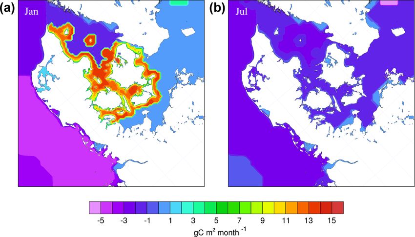
1508                                                A. S. Lansø et al.: CO2 across the heterogeneous landscape of Denmark

updated values every third hour. Similarly, CT2015 3-hourly        polation was conducted between the hourly time steps when
mole fractions of CO2 were read in as boundary conditions          DEHM was reading the hourly meteorological data. Further-
at the lateral boundaries of the main domain.                      more, a correction of the horizontal wind speed was con-
   Hourly anthropogenic emissions on a 10 km × 10 km grid          ducted in DEHM to ensure mass conservation and compli-
from the Institute of Energy Economics and Rational En-            ance with surface pressure (Bregman et al., 2003).
ergy Use (IER, Pregger et al., 2007) were applied for Eu-
rope instead of emissions from CT2015. Furthermore, these          3.1.4   Evaluation of meteorological drivers
are, for the area of Denmark, substituted by hourly anthro-
pogenic emissions with an even higher spatial resolution of        We did not have access to measurements from official mete-
1 km × 1 km (Plejdrup and Gyldenkærne, 2011). As the Eu-           orological observational sites. Thus, for the evaluation of the
ropean and Danish emission inventories were from 2005 and          meteorological drivers, measurements from different types of
2011, respectively, the emissions were scaled to annual na-        monitoring sites were used, comprised of three air pollution
tional total CO2 emissions of fossil fuel and cement produc-       monitoring sites, three FLUXNET sites, and three sites from
tion conducted by EDGAR (Olivier et al., 2014) in order to         the Danish Hydrological Observatory (HOBE; Table 1).
include the yearly variability in national anthropogenic CO2          Wind directions, investigated by comparing wind roses
emissions.                                                         made from WRF outputs and measurements, were at most
                                                                   sites reasonably captured by WRF (see Figs. S1–S3 in the
3.1.2   Air–sea CO2 exchange                                       Supplement). At several sites the frequency of wind direc-
                                                                   tions from the west were overestimated by WRF, mainly at
The exchange of CO2 between the atmosphere and the ocean,          the expense of southern winds. However, the opposite was
FCO2 , was calculated by FCO2 = Kk660 1pCO2 , where K is           the case at Aarhus, where the effect of street canyons was
solubility of CO2 calculated as in Weiss (1974), k660 is the       likely causing higher occurrences from due west in the ob-
transfer velocity of CO2 normalised to a Schmidt number of         served wind directions. The wind velocities were in general
660 at 20 ◦ C, and 1pCO2 is the difference in partial pressure     overestimated by WRF with an average of 1.1 m s−1 , with
of CO2 between the surface water and the overlying atmo-           the greatest differences at the same sites experiencing most
sphere. The transfer velocity parameterisation k = 0.266u210 ,     problems in reproducing the observed wind direction pat-
where u210 is the wind speed at 10 m, determined by Ho et al.      terns (Fig. 2). Moreover, at the Risø campus tower site the
(2006), has been found to match Danish fjord systems (Mørk         wind velocities were underestimated.
et al., 2016) and was applied in the current study. Surface val-      Only one site had available surface pressure measure-
ues of marine pCO2 were described by a combination of the          ments, and high correlation of R 2 = 0.99 was obtained with
open-ocean surface water climatology of pCO2 by Takahashi          the simulation surface pressures, indicating that WRF was
et al. (2014) and the climatology developed by Lansø et al.        capable of reproducing the actual pressure system across the
(2015, 2017) for the Baltic Sea and Danish waters. Further-        study region (Fig. S4). Comparisons of wind velocities and
more, short-term temporal variability was accounted for in         wind rose likewise indicate that WRF captured the general at-
the surface water pCO2 by imposing monthly mean diurnal            mospheric flow patterns, though the overestimated wind ve-
cycles onto the monthly climatologies following the method         locities might induce atmospheric mixing too quickly. The
described in Lansø et al. (2017).                                  simulated mixing layer heights have previously been evalu-
                                                                   ated, and although the diurnal boundary layer dynamics were
3.1.3   Meteorological drivers                                     reproduced together with the rectifier effect, problems with
                                                                   accurately modelling the nighttime boundary layer were ob-
The necessary meteorological parameters for DEHM were              served, possibly overestimating nighttime surface concentra-
simulated by the WRF (Skamarock et al., 2008), nudged by           tions of CO2 (Lansø, 2016). Moreover, long-range transport
6-hourly ERA-Interim meteorology (Dee et al., 2011) for the        and boundary conditions of atmospheric CO2 concentrations
period 2008 to 2014, and were also used as initial and bound-      have previously been shown to be captured by the model sys-
ary conditions. In WRF the Noah land surface model, the            tem across northern Europe, where the current study area
Eta similarity surface layer and the Mellor–Yamada–Janjic          is positioned, using observations from Mace Head, Pallas,
boundary layer scheme were chosen to simulate surface and          Westerland, the oil and gas platform F3, Lutjewad, and Öster-
boundary layer dynamics. The CAM scheme was used for               garnsholm (Lansø et al., 2015).
long- and short-wave radiation, the WRF single-moment                 When evaluating the meteorological variable also impor-
five-class microphysics scheme was applied for microphysi-         tant for the biospheric model component, the surface tem-
cal processes, and the Kain–Fritsch scheme was used for cu-        perature showed high correlation with R 2 above 0.93 for all
mulus parameterisation (Skamarock et al., 2008). In WRF            sites (Fig. 3). The total short-wave incoming radiation (Rin )
the same nests were chosen as in DEHM, and the meteoro-            mirrors the measured Rin from the three HOBE sites but is
logical outputs were saved every hour. To get the sub-hourly       overestimated during summer by WRF (Fig. S5). The val-
values that match the time step in DEHM, a temporal inter-         ues of photosynthetic active radiation (PAR) passed to SPA

Biogeosciences, 16, 1505–1524, 2019                                                    www.biogeosciences.net/16/1505/2019/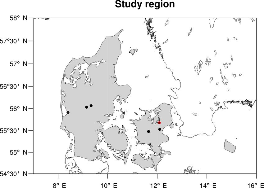
A. S. Lansø et al.: CO2 across the heterogeneous landscape of Denmark                                                                 1509

Table 1. Location of the sites used for evaluation of the meteorological drivers together with the time period from which measurements
are used and the meteorological variables (Met var.) included in the analysis. The measurements were obtained from Danish Hydrological
Observatory (HOBE), FlUXNET and Department of Environmental Science at Aarhus University (AU).

                      Site                   Location               Time period    Met var.              Data source
                      Gludsted               56◦ 040 N, 9◦ 200 E    2009–2014      T2, WS, WD, Rin       HOBE
                      Risbyholm              55◦ 320 N, 12◦ 060 E   2004–2008      T2, WS, WD            FLUXNET
                      Skjern Enge            55◦ 550 N, 8◦ 240 E    2009–2014      T2, WS, WD, Rin       HOBE
                      Sorø                   55◦ 290 N, 11◦ 390 E   2006–2014      T2, WS, WD, SRF       FLUXNET
                      Voulund                56◦ 020 N, 9◦ 090 E    2009–2014      T2, WS, WD, Rin       HOBE
                      Risø campus tower      55◦ 420 N, 12◦ 050 E   2015           T2, WS, WD            FLUXNET
                      Ålborg                 56◦ 020 N, 9◦ 090 E    2004–2015      T2, WS, WD            AU
                      Aarhus                 56◦ 020 N, 9◦ 090 E    2004–2015      T2, WS, WD            AU
                      Copenhagen             56◦ 020 N, 9◦ 090 E    2004–2015      T2, WS, WD            AU

Figure 2. Scatter plots of measured versus modelled 10 m wind velocity for the nine sites used for evaluation of the meteorological drivers.
Hourly average values are used for both simulated and measured wind velocities. Observed average wind velocity (Obs), simulated average
wind velocity (Mod), correlation squared (R 2 ), root-mean-square error (RMSE) and bias are shown for each site.

www.biogeosciences.net/16/1505/2019/                                                             Biogeosciences, 16, 1505–1524, 2019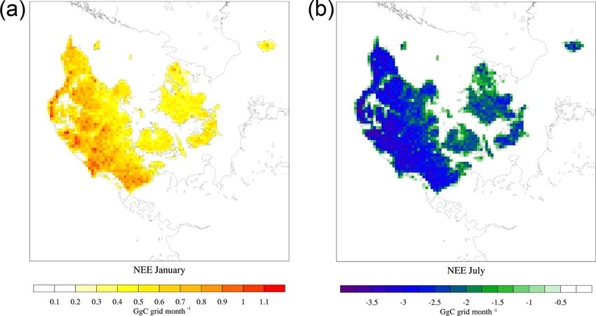
1510                                                  A. S. Lansø et al.: CO2 across the heterogeneous landscape of Denmark

Figure 3. Scatter plots of measured versus modelled 2 m temperatures for the nine sites used for evaluation of the meteorological drivers.
Hourly average values are used for both simulated and measured temperatures. Observed average 2 m temperature (Obs), simulated 2 m
temperature (Mod), correlation squared (R 2 ), root-mean-square error (RMSE) and bias are shown for each site.

from DEHM might thus be overestimated, as PAR is propor-               variation in the vertical profile of photosynthetic parameters
tional to Rin . However, in SPA there is a cap on the limiting         and multi-layer turbulence (Smallman et al., 2013). Within
carboxylation rate in the calculation of the photosynthesis,           the soil, up to 20 soil layers can be simulated (Williams et al.,
and the effect of the overestimated PAR can thus be limited.           2001). The radiative transfer scheme estimates the distribu-
Precipitation was lacking from all sites, but the annual accu-         tion of direct and diffuse radiation and sunlit and shaded
mulated modelled precipitation at the nine sites follows the           leaf areas (Williams et al., 1998). SPA uses the mechanis-
countrywide annual estimates (Cappelan et al., 2018), how-             tic Farquhar model (Farquhar and von Caemmerer, 1982) of
ever, with higher values for the westernmost sites, since              leaf-level photosynthesis and the Penman–Monteith model to
many frontal systems enter Denmark from the west (Fig. S6).            represent leaf-level transpiration (Jones, 1992). Photosynthe-
                                                                       sis and transpiration are coupled via a mechanistic model of
3.2    SPA                                                             stomatal conductance, where stomatal opening is adjusted to
                                                                       maximise carbon uptake per unit of nitrogen within hydraulic
SPA is a mechanistic terrestrial biosphere model (Williams             limitations, determined by a minimum leaf water potential
et al., 1996, 2001). SPA has a high vertical resolution with           tolerance, to prevent cavitation.
up to 10 canopy layers (Williams et al., 1996), allowing for

Biogeosciences, 16, 1505–1524, 2019                                                          www.biogeosciences.net/16/1505/2019/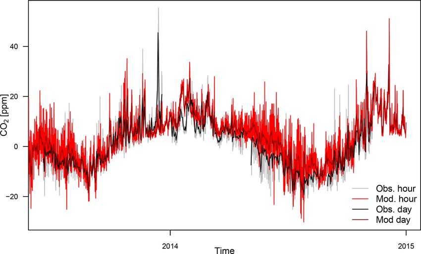
A. S. Lansø et al.: CO2 across the heterogeneous landscape of Denmark 1511
Table 2. Location, species and land cover classification in the model system for the five Danish eddy covariance (EC) sites used for calibration
and validation of SPA.
Site Location Calibration Validation Species LU in SPA–DEHM Reference
Gludsted 56◦ 040 N, 9◦ 200 E 2009–2012 2013–2014 Norway spruce Evergreen forest HOBE
Risbyholm 55◦ 320 N, 12◦ 060 E 2004–2008 – Winter wheat Winter wheat and winter crops FLUXNET
Skjern Enge 55◦ 550 N, 8◦ 240 E 2009–2012 2013–2014 Grass Grassland HOBE
Sorø 55◦ 290 N, 11◦ 390 E 2006–2012 2013–2014 Beech Deciduous forest FLUXNET
Voulund 56◦ 020 N, 9◦ 090 E 2009–2012 2013–2014 Spring and winter barley Spring or winter barley HOBE
Ecosystem carbon cycling and phenology is determined lowing for a better representation of the Danish surface and
by a simple carbon cycle model (DALEC; Williams et al., hence also the biospheric fluxes.
2005), which is directly coupled to SPA. DALEC simulates On an hourly basis, DEHM provides atmospheric CO2
carbon stocks in foliage, fine roots, wood (branches, stems concentrations and the meteorological drivers obtained from
and coarse roots), litter (foliage and fine roots) and soil or- WRF to SPA, while SPA returns net ecosystem exchange
ganic matter (including coarse woody debris). Photosynthate (NEE) to DEHM each hour.
is allocated to autotrophic respiration and living biomass via
fixed fractions, while turnover of carbon pools is governed 3.2.1 SPA calibration
by first order kinetics. In addition, when simulating crops, a
storage organ (i.e. the crop yield) and foliage pools that are The calibration was conducted by selecting a set of inputs
dead but still standing are added, influencing both radiative parameters (plant traits, carbon stocks, etc.), and for each
transfer and turbulent exchange (Sus et al., 2010). parameter, five values within a realistic range were chosen.
SPA has been extensively validated against site observa- Next, 200 SPA simulations with randomly chosen parameter
tions from temperate forests (Williams et al., 1996, 2001), values were conducted. These results were statistically eval-
temperate arable agriculture (Sus et al., 2010) and the Arctic uated against observations of NEE from the different flux
tundra (Williams et al., 2000). SPA has more recently been sites, with the aim of selecting the parameter combination
coupled to the Weather Research and Forecasting (WRF) with the lowest root-mean-square error (RMSE) in combi-
model (Skamarock et al., 2008), and the resulting WRF–SPA nation with highest correlation that captured the observed
model was used in multi-annual simulations over the United variability and onset of the growing season. However, it was
Kingdom and assessed against surface fluxes of CO2 , H2 O not always possible to have all these conditions satisfied (e.g.
and heat, and atmospheric observations of CO2 from aircraft Fig. S7). Based on this random parameter testing, it was pos-
and a tall tower (Smallman et al., 2013, 2014). sible to choose the best set of realistic vegetation input pa-
SPA needs vegetation and soil input parameters. Initial soil rameters that could improve the model performance at the
carbon stock estimates were obtained from the Regridded Danish sites. The best found vegetation parameters values
Harmonized World Soil Database (Wieder, 2014). The vege- corresponded in some cases to the values already applied in
tation inputs and plant traits for SPA were partly taken from SPA for the given land cover.
previous parameter sets used in SPA but also from the Plant
Trait Database (TRY; Kattge et al., 2011) and from literature 3.2.2 SPA evaluation
(Penning de Vries et al., 1989; Wullschleger, 1993). As these
parameters and plant traits were determined at various sites Comparing to observations of NEE, SPA was, in general,
that do not necessarily correspond to Danish conditions, a able to capture the phenology and seasonal cycle through-
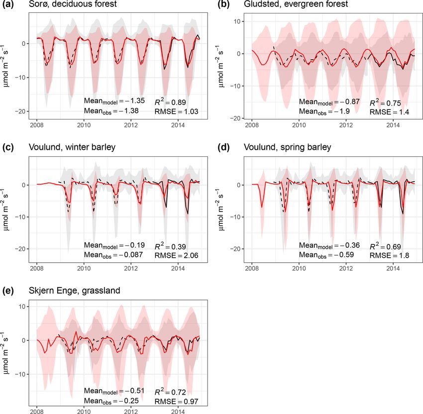
calibration of the vegetation inputs to SPA was conducted for out the entire simulation period (Fig. 4). Correlations and
Danish eddy covariance (EC) flux sites (Table 2). Only data RMSEs between the model and the independent data from
from five sites were available, and these were divided in two the validation period (Fig. 4) likewise indicate a good model
sets – one for calibration (all available observations before performance. At Sorø, variability, as inferred from the stan-
2013) and the other for validation (all available observations dard deviations, the amplitude and the onset of the growing
from 2013 and 2014). season were reproduced well by SPA. However, difficulties
In the innermost nest of DEHM for the area of Denmark, with simulating the evergreen forest at Gludsted are evident,
a coupling was made between DEHM and SPA. Thus, the with more variation modelled than given by the observations
coarser optimised biospheric fluxes from CT2015 were, for and a lag of the start of the growing season when compared to
Denmark, replaced by hourly SPA simulated CO2 fluxes. the observations. The evergreen plant functional type in SPA
With this change, the spatial resolution for the biosphere lacks a labile or non-structural carbohydrate store needed to
fluxes was increased from 1◦ × 1◦ to 5.6 km × 5.6 km, al- drive rapid leaf expansion with the onset of spring; instead
leaf expansion is dependent on available photosynthate in a
www.biogeosciences.net/16/1505/2019/ Biogeosciences, 16, 1505–1524, 2019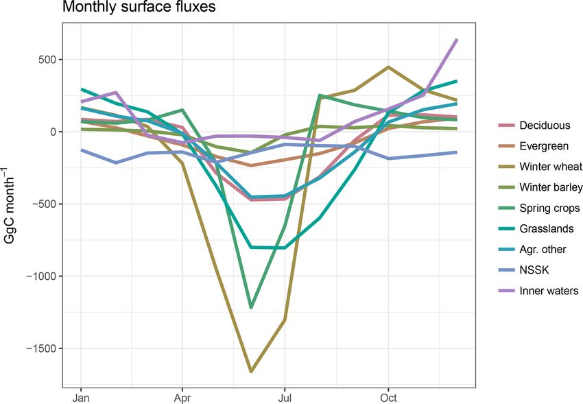
1512                                                 A. S. Lansø et al.: CO2 across the heterogeneous landscape of Denmark

given time step. Therefore, SPA’s leaf area index (LAI) is          Table 3. Statistic metrics for the validation period (2013–2014) for
lower early in the growing season, resulting in a biased slow       the fives sites that have measurements of NEE during the valida-
photosynthetic activity and an underestimation in the mag-          tion period for hourly, daily and monthly values. Measured mean
nitude of NEE, as seen at Gludsted (Fig. 4). Voulund alter-         (meanobs ), modelled mean (meanmodel ), correlation squared (R 2 )
nates between winter and spring barley for the calibration pe-      and root-mean-square error (RMSE) are shown for each site and
                                                                    temporal resolution.
riod starting with winter barley in 2009. Note that the whole
observed time series of NEE at Voulund is shown together
                                                                                           meanobs   meanmodel    R2    RMSE        n
with model NEE of both winter and spring barley (Fig. 4c
and d). While the phenology and amplitude are captured               Deciduous forest

well for spring barley at Voulund, SPA is not able to cap-           Sorø hourly            −1.61       −1.62    0.61    5.17   13 746
                                                                     Sorø daily             −1.58       −1.57    0.66    2.08      587
ture the seasonal amplitude of the winter barley that seems
                                                                     Sorø monthly           −1.38       −1.35    0.89    1.03       21
to be more sensitive to the meteorological drives, and sea-
                                                                     Evergreen forest
sons with harder winters had lower NEE peaks in summer
(winter 2010–2011 and 2012–2013). At the grassland site              Gludsted hourly        −1.95       −0.88    0.59    6.71   17 471
                                                                     Gludsted daily         −1.96       −0.88    0.29    2.31      728
Skjern Enge, NEE is reasonably modelled for winter, spring
                                                                     Gludsted monthly       −1.95       −0.87    0.75    1.41       24
and the first part of the summer. The difficulties for late sum-
                                                                     Winter barley
mer and autumn arise from the management practices at the
site, where both grazing and grass cutting are conducted, lim-       Voulund hourly         −0.09       −0.19    0.39    4.37    8759
                                                                     Voulund daily          −0.09       −0.19    0.33    2.54     365
iting NEE (Herbst et al., 2013). Although grazing is included
                                                                     Voulund monthly        −0.09       −0.19    0.39    2.06      12
in SPA, it does not simulate the same reduction in NEE.
                                                                     Spring barley
   Examining the performance of SPA at a higher temporal
resolution (Table 3), the correlations are better for hourly val-    Voulund hourly         −0.59       −0.36    0.47    5.00    8712
                                                                     Voulund daily          −0.59       −0.36    0.55    2.56     363
ues than daily for the land cover classification having prob-        Voulund monthly        −0.59       −0.36    0.69    1.95      12
lems with the phenology (evergreen forest and winter barley)
                                                                     Grasslands
because SPA is capable of reproducing the diurnal variability.
For the remaining land cover classifications, R 2 and RMSE           Skjern Enge hourly     −0.26       −0.52    0.40    6.18   17 494
                                                                     Skjern Enge daily      −0.26       −0.52    0.25    2.05      729
are improved when going from hourly to monthly averages              Skjern Enge monthly    −0.25       −0.51    0.72    0.97       24
of NEE. Zooming in on shorter time windows, the timing of
the diurnal cycle is in accordance with measured NEE (see
e.g. Fig. S9), but the amplitude is underestimated by SPA.
                                                                    represented well in western Jutland, and even though these
                                                                    land cover classes have gross primary production (GPP), they
4     Results                                                       are still dominated by total ecosystem respiration, but their
                                                                    total ecosystem respiration can be higher than the other land
The model system was run from 2008 to 2014, with the first
                                                                    cover classifications because of the contribution from the au-
3 years regarded as a spin-up period. In the following sec-
                                                                    totrophic respiration that depends on GPP in SPA. During
tions the terrestrial and marine surface fluxes will be pre-
                                                                    July, the productivity is at its highest for all land cover classes
sented first, followed by measurements of atmospheric CO2
                                                                    dominating total ecosystem respiration, resulting in negative
from the Risø campus tower that will be used to assess the
                                                                    NEE (Fig. 6), and the gradient across the country is more
performance of the DEHM–SPA system and evaluate local
                                                                    likely to be a result of the urbanisation.
impacts from fjord systems on atmospheric CO2 concentra-
                                                                       Figure 6 shows the average monthly contribution from
tions.
                                                                    each land cover classification to the countrywide NEE, which
4.1     Surface fluxes                                              inherently follows their productivity but also reflects the area
                                                                    covered by each land cover type, with highest peaks for win-
4.1.1    Biospheric fluxes                                          ter wheat and grasslands during June. During winter, the
                                                                    spread amongst the land cover classifications is smaller but
As shown in Fig. 5, SPA simulates an east–west gradient in          still has numerically larger monthly fluxes for the land cover
NEE for both January and July in 2011. Larger values of             classifications with largest area. Integrating over all land
NEE are found in the western part of Denmark, while the             cover classifications, the Danish terrestrial land surfaces are
islands and eastern Jutland have lower biosphere fluxes. This       a net source of CO2 to the atmosphere in the months from
gradient follows the distribution of the individual land cover      October to April, with the highest release of 1063±154 GgC
classifications (Fig. S8), their phenology and productivity but     per month in December. From May to September, the bio-
also reflects the urbanisation, which is denser in the eastern      sphere is a net sink with a maximum uptake in June of
part of the country. During January, total ecosystem respi-         −4982 ± 385 GgC. The total surface exchange of CO2 be-
ration dominates NEE. Evergreen forests and grasslands are          tween the atmosphere and Danish biosphere is −7337 ±

Biogeosciences, 16, 1505–1524, 2019                                                        www.biogeosciences.net/16/1505/2019/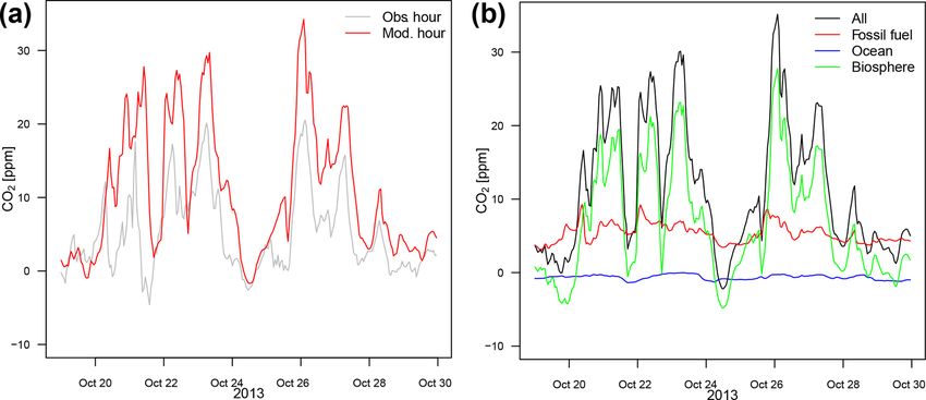
A. S. Lansø et al.: CO2 across the heterogeneous landscape of Denmark                                                             1513

Figure 4. Monthly averaged values of measured (black dashed, calibration period; black solid, validation period) and simulated (red) net
ecosystem exchange (NEE) for the Danish EC sites with measurements in the simulation period. The shaded areas show the standard
deviations for the modelled and measured NEE calculated using hourly fluxes. The model mean (Meanmodel ), observational mean (Meanobs ),
correlation squared (R 2 ) and root-mean-square error (RMSE) for the validation period (2013 and 2014) are shown for each site.

1468 GgC yr−1 , where winter wheat has the largest contri-            While the North Sea area contained within the EEZ continu-
bution with −2342 ± 1045 GgC yr−1 .                                   ously had uptakes in the range −73 to −191 GgC per month
                                                                      with an accumulation of 1765 GgC yr−1 , the fluxes from the
4.1.2   Marine fluxes                                                 near-coastal Danish inner waters varied in the range −46 to
                                                                      540 GgC per month, releasing 1343 GgC yr−1 to the atmo-
The air–sea CO2 exchange in the Danish inner waters expe-             sphere.
riences large seasonal variations, while the variations in the
North Sea are less pronounced, as illustrated by Fig. 7. The          4.2   Atmospheric CO2 concentrations
mineralisation in winter increases the surface water pCO2 in
the Danish inner waters, resulting in outgassing of CO2 to the        The time series of measured and simulated CO2 show good
atmosphere, while uptake occurs during spring and summer              agreement (Fig. 8) with R 2 = 0.77 and RMSE = 4.87 ppm
months following the decrease in surface water pCO2 due to            for daily averaged time series, demonstrating that the model
biological activities.                                                is capable of capturing the synoptic scale variability. Also,
   The simulated annual air–sea CO2 exchange in the                   good statistical measures are obtained for the hourly time se-
105 000 km2 covered by the Danish EEZ amounts to                      ries with R 2 = 0.71 and RMSE = 5.95 ppm, but the short-
−422 GgC yr−1 . However, this number masks large spatial              term variability was not always fully captured by the model.
differences and monthly numerical larger fluxes (Fig. 6).             All in all, the evaluation shows that the model can capture

www.biogeosciences.net/16/1505/2019/                                                          Biogeosciences, 16, 1505–1524, 2019
1514 A. S. Lansø et al.: CO2 across the heterogeneous landscape of Denmark
Figure 5. Net ecosystem exchange (NEE) for January (a) and July (b) 2011.
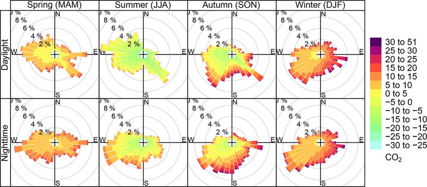
est values are obtained in particular during daylight, when
photosynthesis occurs.
The individual contribution from fossil fuel emissions,
marine and biospheric exchanges to the atmospheric CO2
(see Figs. S11–S13) indicate that the biosphere contributes
most to the variations simulated at Risø (Fig. S12) – both sea-
sonally and daily. Emissions of fossil fuel experience little di-
urnal variability, but seasonally having the greatest contribu-
tion during autumn and winter (Fig. S11). The highest values
are seen originating from the sectors encapsulating the city of
Roskilde and the capital region. In all seasons, the simulated
oceanic contribution is negative, i.e. indicating uptake of at-
mospheric CO2 , but the marine contribution is small, with
little variation (Fig. S13). The less negative values in autumn
and winter may be a result of the simulated outgassing of
Figure 6. Total monthly average of NEE for each land cover clas-
CO2 from the Baltic Sea and Danish inner waters during the
sification for the simulation period of 2011–2014 together with the
winter season (Lansø et al., 2015), which, however, is still
monthly air–sea CO2 from the Danish marine areas that have been
divided into the North Sea and Skagerak (NSSK) and Kattegat and dominated by the uptake by global open oceans.
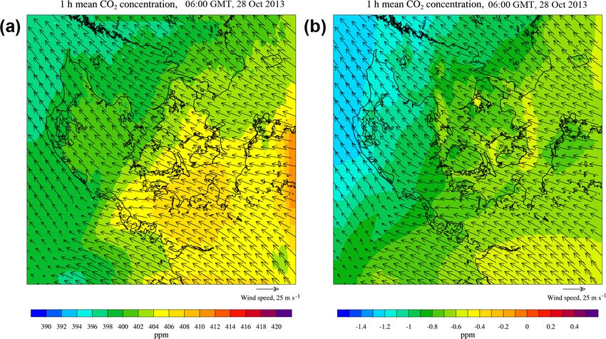
the Danish straits (inner waters). The local impact from Roskilde Fjord is difficult to de-
tect in the marine concentration plots. Flux measurements
at Roskilde Fjord have shown uptake of CO2 during spring
while release of CO2 in the remaining seasons (Mørk et al.,
the overall variability in the atmospheric CO2 concentra- 2016), which is accurately captured by the modelling system
tions and fluxes. Moreover, the higher resolution in both the (Lansø et al., 2017). A footprint analysis of the Risø tower
transport model and surface fluxes results in a better model has shown that the fluxes from Roskilde Fjord have a contri-
performance in simulating atmospheric CO2 concentrations bution to the total CO2 flux measured at the top of the 118 m
(Fig. S10). high tower, but it is only minor, since fluxes over water are
To investigate the origin of the CO2 simulated at the Risø typically an order of magnitude smaller than fluxes over land
site, concentration rose plots of simulated atmospheric CO2 (Sogachev and Dellwik, 2017). Therefore, we investigated a
have been made (Fig. 9). The concentration rose shows the period with observed large outgassing from Roskilde Fjord
wind direction and associated CO2 concentrations. Division – a storm event in October 2013 that was observed to in-
has been made between seasons and daytime and nighttime crease the monthly release of CO2 in the fjord by 66 % (Mørk
values, both showing distinct seasonal and diurnal patterns. et al., 2016). The storm event passed Denmark on 28 Oc-
The highest values of CO2 are obtained during winter, where tober 2013, and at 06:00 UTC southerly winds transport air
very little diurnal variation is seen. During summer the low-
Biogeosciences, 16, 1505–1524, 2019 www.biogeosciences.net/16/1505/2019/A. S. Lansø et al.: CO2 across the heterogeneous landscape of Denmark 1515
Figure 7. Simulated air–sea CO2 exchange within the model framework for January (a) and July (b) 2011. The spatial resolution follows
those of nest 4 from the DEHM model (i.e. 5.6 km × 5.6 km). The formulation by Ho et al. (2006) was used to calculate the air–sea CO2
exchange.
5 Discussion
5.1 Surface fluxes
The simulated annual uptake by deciduous forest of −284 ±
21 gC m−2 yr−1 for the period 2011–2014 is within the ob-
served range of annual estimated NEE at Sorø from 1996
to 2009, spanning from 32 to −331 gC m−2 yr−1 (Pilegaard
et al., 2011). Improvements to the evergreen plant functional
type in SPA are needed, and an addition of a labile pool
to the evergreen carbon assimilation would omit the sea-
sonal lag (Williams et al., 2005). Such adjustments have al-
ready been made to the DALEC carbon assimilation system
Figure 8. Hourly averages and daily averages of modelled and con-
utilised by SPA (Smallman et al., 2017), substantially im-
tinuously measured atmospheric CO2 at the Risø site for 2013– proving the representation of terrestrial phenology but not
2014. The trends have been removed from the time series. yet being incorporated into SPA. The estimated uptake of
−355 ± 41 gC m−2 yr−1 is in the low range of previous esti-
mates of temperate evergreen forests with −402 gC m−2 yr−1
masses with higher CO2 towards the Risø site (Fig. 10a), (Luyssaert et al., 2007) and Danish evergreen plantations
while at the same time a detectable increase in the oceanic of −503 gC m−2 yr−1 (Herbst et al., 2011). This could be
contribution to the CO2 concentration at the Roskilde Fjord caused by the slow leaf onset in spring, inhibiting the pro-
system is seen (Fig. 10b). The model system simulates the ductivity at the beginning of the growing season.
small peak in the observed atmospheric CO2 concentrations Previous annual estimates at Danish agricultural field
for 28 October (Fig. 11a) at the Risø site, but distinguish- sites found carbon uptake of −31 gC m−2 yr−1 esti-
ing between contributions from fossil fuel emissions, the mated from a mixed agricultural landscape (Soegaard
biosphere and the ocean to the atmospheric CO2 concentra- et al., 2003) and −245 gC m−2 yr−1 at a winter bar-
tion at Risø (Fig. 11b) reveals no oceanic impact, and hence ley site (Herbst et al., 2011). The SPA–DEHM model
there is no apparent influence from Roskilde Fjord during the system simulated annual uptakes for winter wheat of
storm event. −252 ± 113 gC m−2 yr−1 , and spring crops of −179 ±
28 gC m−2 yr−1 , while winter barley had a smaller uptake of
−82 ± 91 gC m−2 yr−1 with large standard deviation poten-
tially resulting in small annual releases. The calibration and
validation (Fig. 4c) show difficulties in simulating the ob-
served NEE during growing seasons for winter barley, par-
www.biogeosciences.net/16/1505/2019/ Biogeosciences, 16, 1505–1524, 20191516 A. S. Lansø et al.: CO2 across the heterogeneous landscape of Denmark Figure 9. Concentration roses of modelled atmospheric CO2 (ppm) at the Risø site for 2011–2014. The wind direction is split into 10◦ intervals, and the frequency is indicated by the concentric circles. The colours indicate the CO2 concentrations with mean removed that have been transported to the site from the given wind directions. Figure 10. (a) Hourly averages of atmospheric CO2 concentrations including the annual background across Denmark on 28 October 2013 06:00 UTC during the October storm. (b) The contribution from the marine exchange alone to the hourly averaged atmospheric CO2 con- centration on 28 October 2013 06:00 UTC. The less negative values at the Roskilde Fjord system indicate release of CO2 to the atmosphere. ticularly after cold and snow-covered winters. As pointed with most sites having an annual uptake of carbon. As seen in out in previous studies, the crop modelling component in Fig. 4e, more work on grassland calibration could have been SPA could likewise be improved, e.g. by inclusion of intra- done, but the conditions and management regimes at Skjern seasonal crops (Smallman et al., 2014). Enge do not necessarily fit the rest of the Danish grasslands. The current study estimated the Danish grasslands to be With the chosen parameters, very comparable results were a sink of CO2 with −210 ± 43 gC m−2 yr−1 , which is sim- obtained, indicating that such an additional calibration might ilar, albeit slightly smaller, than the −267 gC m−2 yr−1 ob- not be advantageous. served at the Skjern Enge grassland site during 2009–2011 A tilling approach has been used for the land cover clas- (Herbst et al., 2013) and the −312 gC m−2 yr−1 observed at sification in the SPA–DEHM modelling framework, includ- the Lille Valby grassland site, Denmark (Gilmanov et al., ing sub-grid heterogeneity in the model system. However, 2007). The European grassland study by Gilmanov et al. the seven land cover classes do not fully encompass the (2007) found large variation in annual fluxes from grassland ecosystem variability in Denmark. Both grassland and agri- driven by environmental conditions and management prac- cultural other cover a broad range of subcategories, with both tices at the sites varying from 171 to −707 gC m−2 yr−1 , but heather and meadow included in the grassland class, while Biogeosciences, 16, 1505–1524, 2019 www.biogeosciences.net/16/1505/2019/
A. S. Lansø et al.: CO2 across the heterogeneous landscape of Denmark                                                             1517

Figure 11. (a) Hourly averages of modelled and continuously measured atmospheric CO2 at the Risø site for 19–29 October 2013 with annual
means removed. (b) Contributions from fossil fuel emission, oceanic surface exchange and biospheric surface exchange to the atmospheric
CO2 concentration, shown as 1 h averages of modelled concentrations at the Risø site for the same period.

agricultural other contains, for example, vegetables fields,          and fossil fuel emissions of CO2 . The signal from Roskilde
hedgerows, woodland patches and uncultivated land, high-              Fjord is difficult to detect in the simulated CO2 concentra-
lighting the need to adopt approaches allowing for generating         tions. Even when the marine contribution to the atmospheric
novel spatially varying parameter sets (Bloom et al., 2016).          concentration alone is examined, the Roskilde Fjord signal
Moreover, large urbanised areas are not accounted for in the          is hard to distinguish at the Risø campus tower. Moreover,
current classes either. Adding more land cover classifications        sea breezes from the narrow Roskilde Fjord might be diffi-
could give a better and more realistic surface description, if        cult to detect by the model system with its 5.6 km horizontal
data for both calibration and validation for the lacking land         resolution.
cover classes, preferably from a similar climatic region to              As Roskilde Fjord previously was found by a footprint
Denmark, were available.                                              analysis to have an impact on the atmospheric CO2 concen-
   Compatible marine fluxes to previous estimates are ob-             tration at the top of the tower (Sogachev and Dellwik, 2017),
tained for the study region. On an annual basis, the Danish           a period with observations of large outgassing from Roskilde
inner waters were found to be a source of 30 gC m−2 yr−1 ,            Fjord was examined to more clearly envision its impact in the
which agrees with most previous studies. Wesslander et al.            simulated concentration fields. Both the simulated and ob-
(2010) estimated Kattegat to act as a small sink of                   served atmospheric CO2 increased during the storm event on
−14 gC m−2 yr−1 based on measurements of water chem-                  28 October (Fig. 10a), but no concurrent increase was seen in
istry, while Norman et al. (2013), on the contrary, found a           the oceanic contribution to atmospheric CO2 at the Risø site
release of 19 gC m−2 yr−1 using a biogeochemical model of             (Fig. 10b). This might be explained by the southerly winds
the Baltic Sea. Measurements from Danish fjords, on the               that transported the CO2 released from the fjord northward
other hand, consistently point towards these marine areas be-         and away from the Risø campus tower, which is positioned
ing annual sources of CO2 , with values in the range of 41            in the southern part of the fjord. Moreover, in this study the
to 104 gC m−2 yr−1 (Gazeau et al., 2005; Mørk et al., 2016).          increased flux from Roskilde Fjord was only caused by in-
The current study estimates the North Sea to be a sink of             creased wind speed together with the imposed diurnal cycle
−29 gC m−2 yr−1 , which is very close to previous estimates,          of marine pCO2 (the diurnal amplitude for October was ap-
both measured and modelled, of −20 and −25 m−2 yr−1                   proximately 10 µatm), while measurements suggested that an
(Thomas et al., 2004; Prowe et al., 2009).                            increase in surface water pCO2 of approximately 300 µatm
                                                                      also sustained the observed CO2 flux (Mørk et al., 2016).
5.2   Atmospheric CO2 and land–sea signals                            The lack of such an increase in surface water pCO2 in the
                                                                      current modelling study could explain why no impact on the
WRF is in general capable of simulating the observed wind             simulated atmospheric CO2 is seen from the marine com-
patterns, while the overestimation of the wind velocity could         ponent during the storm event. Thus, the results could indi-
lead to an overestimation of the atmospheric mixing. How-             cate that (i) the narrow Roskilde Fjord was not sufficiently
ever, the SPA–DEHM modelling system resembles the syn-                resolved in the current model framework, where the horizon-
optic and diurnal variability in the atmospheric CO2 concen-          tal grid resolution is 5.6 km × 5.6 km, (ii) the surface water
trations measured at Risø campus tower site. The variabil-            pCO2 was not described in enough detail in the model sys-
ity at the Risø site is dominated by the biospheric impact            tem, (iii) Roskilde Fjord is not in the footprint of the tower

www.biogeosciences.net/16/1505/2019/                                                          Biogeosciences, 16, 1505–1524, 2019
1518 A. S. Lansø et al.: CO2 across the heterogeneous landscape of Denmark
during the storm event or (iv) the fjord only has a minor im- rent study, since the terrestrial surface fluxes in this study are
pact on the atmospheric CO2 concentrations at Risø. constrained by one data stream consisting of EC measure-
However, the air–sea CO2 exchange from the Danish in- ments. This study has focussed on surface fluxes over a rela-
ner waters (including all fjord, inner straits and Kattegat) has tive short time period, and the model framework was capable
an impact during winter. Between November and February, of producing such fluxes, including their aggregated impact
the air–sea fluxes from the Danish inner water correspond to on atmospheric CO2 concentrations (Fig. 4) with R 2 = 0.77
23 %–60 % of the monthly NEE (see Fig. 6). Moreover, the and RMSE = 4.87 ppm for daily values.
higher values of about 0.5 ppm in the concentration roses of Uncertainties of the marine fluxes can be associated with
the marine contribution to the atmospheric CO2 concentra- both the choice of transfer velocity parameterisation, choice
tions at the Risø campus tower site in winter likewise empha- of the wind speed product and the used surface water pCO2
sise the marine impact, though the outgassing from the neigh- maps. Sensitivity analysis of global transfer velocity param-
bouring Baltic Sea also has a contribution. Although the an- eterisation based on 14 C bomb inventories shows uncertain-
nual total numerical marine fluxes of 1765 gC yr−1 from the ties of 20 %, while varying the applied wind speed products
North Sea and 1343 gC yr−1 from the Danish inner waters for these formulation increases the difference in the global
are comparable to the sizes of annual NEE for individual land annual flux by 40 % (Roobaert et al., 2018). Including em-
cover classifications (e.g. deciduous at −987 gC yr−1 , ever- pirical formulations of transfer velocity parameterisation in
green at −665 gC yr−1 and grasslands at −1467 gC yr−1 ), the the analysis increased the sensitivity of the wind speed prod-
air–sea CO2 fluxes are 1 order of magnitude smaller than uct to nearly 70 %, while the uncertainty of the parameterisa-
the biospheric fluxes, with 30 gC m−2 yr−1 for the Danish in- tion itself rose to more than 200 %. More than a doubling of
ner waters and −29 gC m−2 yr−1 for the North Sea and Sk- the annual uptake by the usage of different transfer velocity
agerak. formulations has likewise been shown for the study region
(Lansø et al., 2015), while the choice of the surface water
5.3 Uncertainties in relation to surface exchanges of pCO2 map could change the study region from an annual
CO2 sink to source of atmospheric CO2 (Lansø et al., 2017). As
shown by Roobaert et al. (2018) the ERA-Interim and the
Some of the largest uncertainties lie in the parameters under- transfer velocity formulation by Ho et al. (2006) used in the
lying the terrestrial carbon cycle, in particular those govern- present study have a combined uncertainty estimate around
ing allocation to plant tissues and their subsequent turnover. 20 %. The improved data-driven near-coastal Danish pCO2
Most often these are based on maps of land cover or plant climatology better reflects the observed spatial dynamics and
functional type, but parameter estimation via data assimila- seasonality in the Danish inner waters (Mørk, 2015), albeit
tion analysis has shown substantial spatial variation in ter- not diminishing the uncertainty related to surface maps of
restrial ecosystem parameters within plant functional type pCO2 but reducing it.
groupings, with consequences for carbon cycling predictions
(Bloom et al., 2016). Increasing the quantity and type of ob-
servations available for data assimilation systems can have a 6 Conclusions
significant impact on reducing uncertainty of model process
parameters and simulated fluxes (Smallman et al., 2017). In By usage of the designed mesoscale modelling framework, it
particular, availability of repeated above-ground biomass es- was possible to get detailed insight into the spatio-temporal
timates was able to half the uncertainty of net biome pro- variability in the Danish surface exchanges of CO2 and the
ductivity estimates for temperate forests (Smallman et al., relative contribution from the different surface types. The
2017). Above-ground biomass estimates are currently avail- simulated biospheric fluxes experienced an east–west gra-
able from remote sensing sources (e.g. Thurner et al., 2014; dient corresponding to the distribution of the land cover
Avitabile et al., 2016), with future planned missions such as classes, their biological activity and the urbanisation pattern
the ESA Biomass mission (Le Toan et al., 2011) and NASA across the country. The relative importance of the seven land
GEDI (https://gedi.umd.edu/, last access: January 2019) pro- cover classes varied throughout the course of the year. Grass-
viding high-quality observations over the tropics and global lands had a high contribution to the monthly NEE through all
scales, respectively. seasons, while croplands influence grew from March to July.
While SPA also uses DALEC to simulate carbon allocation On an annual basis, winter wheat had the largest impact on
and turnover, it is currently impractical to conduct a simi- the biospheric uptake, with −2342 GgC yr−1 . However, the
lar data assimilation analysis to optimise DALEC (or SPA) simulated biospheric uptake could benefit both from model
parameters based on comparison with observations of atmo- improvement and divisions into more land cover classes. The
spheric CO2 concentrations, as this would require repetition marine fluxes, being subdivided into the North Sea including
of computationally intense simulations of atmospheric trans- Skagerak and the Danish inner waters, had annual fluxes of
port. While conducting such an analysis remains a future opposite signs, with the North Sea being a continuous sink of
ambition, we consider it to be out of the scope of the cur- atmospheric CO2 and the Danish inner waters experiencing
Biogeosciences, 16, 1505–1524, 2019 www.biogeosciences.net/16/1505/2019/You can also read