Wave-sea-ice interactions in a brittle rheological framework
←
→
Page content transcription
If your browser does not render page correctly, please read the page content below
The Cryosphere, 15, 431–457, 2021
https://doi.org/10.5194/tc-15-431-2021
© Author(s) 2021. This work is distributed under
the Creative Commons Attribution 4.0 License.

Wave–sea-ice interactions in a brittle rheological framework
Guillaume Boutin1 , Timothy Williams1 , Pierre Rampal2,1 , Einar Olason1 , and Camille Lique3
1 Nansen  Environmental and Remote Sensing Center and the Bjerknes Centre for Climate Research, Bergen, Norway
2 CNRS,  Institut de Géophysique de l’Environnement, Grenoble, France
3 Univ. Brest, CNRS, IRD, Ifremer, Laboratoire d’Océanographie Physique et Spatiale, IUEM, Brest 29280, France

Correspondence: Guillaume Boutin (guillaume.boutin@nersc.no)

Received: 14 January 2020 – Discussion started: 24 January 2020
Revised: 1 October 2020 – Accepted: 11 November 2020 – Published: 28 January 2021

Abstract. As sea ice extent decreases in the Arctic, surface       1   Introduction
ocean waves have more time and space to develop and grow,
exposing the marginal ice zone (MIZ) to more frequent and
more energetic wave events. Waves can fragment the ice             The interactions between ocean surface waves and sea ice
cover over tens of kilometres, and the prospect of increas-        have been receiving a significant amount of attention in re-
ing wave activity has sparked recent interest in the interac-      cent years, particularly motivated by the decreasing Arctic
tions between wave-induced sea ice fragmentation and lat-          sea ice extent (Meier, 2017) resulting in larger areas of open
eral melting. The impact of this fragmentation on sea ice          water exposed to the wind and thus available for wave gen-
dynamics, however, remains mostly unknown, although it is          eration. As a consequence, wave events in the Arctic are ex-
thought that fragmented sea ice experiences less resistance        pected to be more frequent and more intense (Thomson and
to deformation than pack ice. Here, we introduce a new cou-        Rogers, 2014) with waves penetrating far into the ice cover
pled framework involving the spectral wave model WAVE-             and breaking large sea ice plates into floes of less than a
WATCH III and the sea ice model neXtSIM, which includes a          few hundred metres (see, e.g. Langhorne et al., 1998; Collins
Maxwell elasto-brittle rheology. This rheological framework        et al., 2015). The attenuation of waves by sea ice, however,
enables the model to efficiently track and keep a “memory”         limits this fragmentation to the interface between the open
of the level of sea ice damage. We propose that the level of       ocean and the pack ice in the so-called marginal ice zone
sea ice damage increases when wave-induced fragmentation           (MIZ). The MIZ is a highly dynamic area characterized by
occurs. We used this coupled modelling system to investi-          strong interactions between the ocean, sea ice and atmo-
gate the potential impact of such a local mechanism on sea         sphere. State-of-the-art sea ice models used in climate pre-
ice kinematics. Focusing on the Barents Sea, we found that         diction systems have been shown to fail at representing the
the internal stress decrease of sea ice resulting from its frag-   complexity of these interactions and have their biggest er-
mentation by waves resulted in a more dynamical MIZ, par-          rors in the MIZ (Tietsche et al., 2014). On shorter timescales,
ticularly in areas where sea ice is compact. Sea ice drift is      large uncertainties remain in the forecasts of the position of
enhanced for both on-ice and off-ice wind conditions. Our          the sea ice edge (Schweiger and Zhang, 2015; DeSilva and
results stress the importance of considering wave–sea-ice in-      Yamaguchi, 2019); however, this information is essential for
teractions for forecast applications. They also suggest that       the safety of the increasing number of human activities in po-
waves likely modulate the area of sea ice that is advected         lar regions (Yumashev et al., 2017). These inaccuracies can
away from the pack by the ocean, potentially contributing to       certainly be attributed (at least in part) to the lack of repre-
the observed past, current and future sea ice cover decline in     sentation of some of the processes occurring in the MIZ and
the Arctic.                                                        the impact of the waves on sea ice dynamics is one of them.
                                                                      Waves can impact sea ice dynamics in the MIZ through
                                                                   a variety of processes. For instance, wave attenuation trans-
                                                                   fers momentum from waves to sea ice through wave radiation
                                                                   stress (WRS, Longuet-Higgins, 1977), which acts as a force

Published by Copernicus Publications on behalf of the European Geosciences Union.
432                                           G. Boutin et al.: Wave–sea-ice interactions in a brittle rheological framework

that pushes the sea ice in the direction of the incident waves.       Modelling efforts relating to waves-in-ice have progressed
Being mostly directed on-ice, its main effect is to maintain a     a lot in recent years, although the heterogeneous nature of
compact sea ice pack near the ice edge, but its importance         sea ice and the wide variety of wave attenuation processes
is still being discussed. Estimating wave attenuation from         in the MIZ still make wave prediction in ice highly chal-
synthetic aperture radar (SAR) images, Stopa et al. (2018b)        lenging (Thomson et al., 2018; Squire, 2018). The impor-
found it to be as important as wind stress over the first 50 km    tance of each wave attenuation process varies with wave and
of the MIZ in the Southern Ocean, whereas Alberello et al.         sea ice properties. Scattering, for instance, is efficient to at-
(2020) did not observe any wave-induced sea ice drift in pan-      tenuate short waves in fragmented sea ice covers made of
cake ice in the Southern Ocean from in situ measurements           consolidated floes (Wadhams et al., 1986; Montiel et al.,
despite a strong wave-in-ice activity. Fragmentation is also       2016), while dissipative mechanisms, like under-ice friction,
likely to change the mechanical properties of the ice, but the     are expected to dominate in the case of forming ice and long
evolution of dynamical and mechanical properties of sea ice        swells propagating in the pack. A sequence of reviews by
cover with floe size remains poorly understood.                    Squire et al. (1995) and Squire (2007, 2020) gave a more de-
   Intuitively, we expect that broken ice is more mobile than      tailed history of this area of work. Liu and Mollo-Christensen
continuous ice (e.g. McPhee, 1980), having lower internal          (1988) and Collins et al. (2015) have stressed the impor-
stress. This seems to be consistent with the deformation ob-       tance of the floe size on wave attenuation. These reports have
servations of Oikkonen et al. (2017) collected by ship radar       motivated the implementation of interactions between waves
during the N-ICE-2015 expedition. In their observations, de-       and floe size, through fragmentation, in numerical models.
formation in fragmented sea ice was an order of magnitude          The first studies used one-dimensional models to look at the
higher than in the pack. However, in the absence of routinely      feedback between ice break-up and wave attenuation (Du-
available datasets providing synoptic information on sea ice       mont et al., 2011; Williams et al., 2013a, b). These models
drift, wave height and floe size in the MIZ, observations do       assume that break-up occurs if wave-induced flexural stress
not allow us to arrive at any explicit relationship between the    overcomes sea ice strength and that the resulting floe size
level of fragmentation and the ability of sea ice cover to be      distribution (FSD) follows a truncated power law with its up-
deformed.                                                          per limit (often called maximum floe size, Dmax ) depend-
   A few attempts have been made to relate floe size to sea        ing on the wave field (Dumont et al., 2011). This assumption
ice dynamics in theoretical models. Shen et al. (1986) used        about the shape of the FSD is based on observations made
a collisional stress term accounting for floe size to repre-       by Toyota et al. (2011) of power-law FSD in the MIZ that
sent sea ice behaviour in the MIZ. The fluctuations of the         they explain by successive fragmentation of floes by waves.
velocity field they obtain, however, did not reproduce obser-      More recently, Boutin et al. (2018) included a parameteriza-
vations from the MIZEX campaigns; they were too small by           tion in the spectral wave model WAVEWATCH III (WW3:
an order of magnitude. Feltham (2005) used a similar colli-        The WAVEWATCH III Development Group, 2019) that also
sional stress but allowed the velocity fluctuations to be time     assumes a power-law FSD. Their parameterization enables
dependent. He showed that it enables the generation of ice         interactions between sea ice floe size and wave attenuation
jets in the MIZ but on smaller scales than the reported ob-        processes, like scattering and inelastic dissipation, and was
servations of ice jets by Johannessen et al. (1983). Dynamics      shown to explain well the wave height evolution during the
in state-of-the-art sea ice models, however, do not account        ice break-up event reported by Collins et al. (2015). Ard-
for the floe size. Instead, the region of the MIZ where sea        huin et al. (2018) evaluated this model by comparing their
ice behaves almost in free drift is mostly a function of sea       results to remote sensing and field measurements during a
ice concentration. The potential impact of fragmentation in        storm event in the Beaufort Sea, showing good agreement
compact ice is therefore neglected, whereas regions of low         for the measured and modelled wave-in-ice attenuation and
sea ice concentration and high wave activity do not neces-         broken sea ice extent. Sea ice representation in these wave
sarily coincide (Horvat et al., 2019). Vichi et al. (2019) anal-   models remains, however, too simplistic to more deeply in-
ysed a cyclone and showed how sea ice in the Antarctic MIZ         vestigate the impact of waves on sea ice. It has led to the
is visibly deformed on sea ice concentration maps despite          development of coupled wave–ice models, first using one-
being highly compact. They stated that this behaviour could        dimensional wave-in-ice models (Williams et al., 2017; Ben-
not be reproduced using a concentration-only criterion to dy-      netts et al., 2017; Bateson et al., 2020; Roach et al., 2018)
namically distinguish pack ice from the MIZ, stressing the         and more recently using more complex spectral wave mod-
need to account for other properties like the floe size. How-      els like WW3 (Boutin et al., 2020; Roach et al., 2019). These
ever, linking floe size, or fragmentation, to sea ice dynamics     developments were made possible by the implementation of
remains a challenging task, first because of the limited data      wave–ice interactions in state-of-the-art sea ice models, par-
available but also due to the poor understanding of the way        ticularly representations of the FSD (Zhang et al., 2015; Hor-
waves propagate in the MIZ, although modelling progress            vat and Tziperman, 2015). These FSDs have been mostly
has been made in this particular field.                            used to investigate the effects of lateral melting on sea ice
                                                                   properties over timescales of a few weeks to a few years in a

The Cryosphere, 15, 431–457, 2021                                                       https://doi.org/10.5194/tc-15-431-2021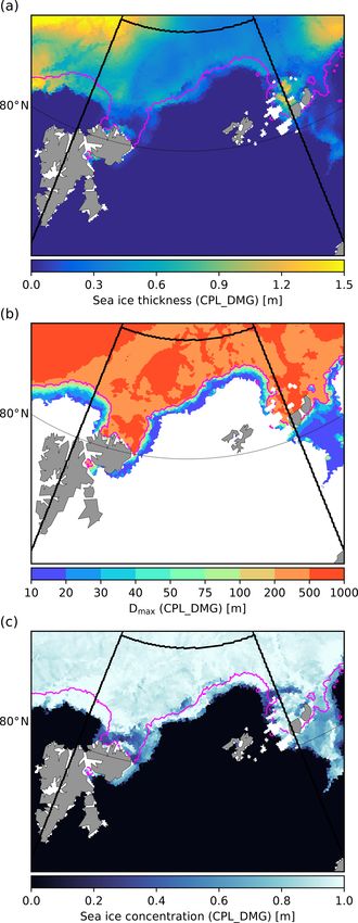
G. Boutin et al.: Wave–sea-ice interactions in a brittle rheological framework                                               433

context where lateral melt is expected to be enhanced by the      scribed by Boutin et al. (2020). We also propose a way to
wave-induced sea ice fragmentation (Asplin et al., 2012).         incorporate some floe size “memory” of previous fragmen-
   The dynamical aspects of wave–ice interactions have re-        tation events due to waves by introducing two time-evolving
ceived less attention. Boutin et al. (2020) found that the WRS    FSDs in each grid cell. These developments provide a cou-
could regionally impact sea ice melt and sea surface prop-        pled wave–sea-ice framework able to provide year-round re-
erties in the Arctic MIZ at the end of summer. Concerning         gional or pan-Arctic simulations. After describing the details
the impact of wave-induced fragmentation, Rynders (2017)          of our implementation, we evaluate our new coupled frame-
suggested combining the classical elasto-visco-plastic rheol-     work to check if the produced wave attenuation, broken sea
ogy used in most sea ice models with a granular rheology in       ice extent and refreezing timescales are reasonable. We then
the MIZ to better represent floe–floe interactions. This gran-    investigate the effects of wave-induced sea ice fragmentation
ular rheology depends on the floe size. Numerical simula-         using a regional case study. Finally, we discuss the different
tions with this approach show an overall increase of the sea      assumptions made in our study and suggest perspectives for
ice drift speed in the Arctic year-round compared to a refer-     future studies.
ence simulation using a standard version of the sea ice model
CICE (Hunke, 2010). Williams et al. (2017) suggested an-
other approach to relate sea ice dynamics to wave-induced         2   Implementation of the coupling between the wave
sea ice fragmentation using the sea ice model neXtSIM (neXt           and sea ice models
generation Sea Ice Model, Rampal et al., 2019) in a stand-
alone set-up. The elasto-brittle (EB) rheology (Girard et al.,    In this study, we make use of the spectral wave model WAVE-
2011) used by neXtSIM stores a variable for sea ice called        WATCH III® (The WAVEWATCH III Development Group,
damage, which tracks the level of mechanical damage of the        2019), building on the previous developments reported by
sea ice over each grid cell (Bouillon and Rampal, 2015; Ram-      Boutin et al. (2018), who included an FSD in WW3 as well as
pal et al., 2016). The higher the damage, the lower the sea       some representations of the different processes by which sea
ice internal stress. Resistance to deformation is a function of   ice can affect the propagation and modulation of waves in the
both sea ice concentration and floe size. The originality of      MIZ. These attenuation processes are scattering (which re-
the study by Williams et al. (2017) was to link the damage        distributes the wave energy without dissipation), friction un-
variable with wave-induced fragmentation, making the ex-          der sea ice (with a viscous and a turbulent part depending on
tension of the ice region behaving in free drift dependent on     the wave Reynolds number) and inelastic flexure. All of these
the wave field. This was done by linking the damage variable      processes depend on sea ice thickness, concentration and floe
with wave-induced fragmentation. Using idealized simula-          size. Wave attenuation increases with thickness and concen-
tions of waves compressing ice, they showed that the move-        tration, and tends to decrease when the floe size is lower than
ment of the ice edge was not very sensitive to either wave        the wavelength, as floes are not flexed anymore. This param-
fragmentation or the WRS. The investigations of Williams          eterization was chosen because it was shown to reproduce
et al. (2017) were, however, limited to very idealized cases,     well wave attenuation in two different events in the Arctic:
and the EB rheology in neXtSIM has now been upgraded to           waves breaking a continuous sea ice cover near Svalbard as
the Maxwell elasto-brittle (MEB) rheology (see Dansereau          reported by Collins et al. (2015) and waves propagating in
et al., 2016), greatly improving sea ice deformation in pack      forming ice in the Beaufort Sea (Ardhuin et al., 2018). As in
ice (Rampal et al., 2019). This upgrade could also affect the     the study by Ardhuin et al. (2018), we assume that deviations
MIZ, as it led to the removal of an ice pressure term that        from the ice-free wave dispersion relationship induced by the
was added to prevent damaged ice from piling up in EB but         presence of ice are small and can be neglected. This is likely
caused the modelled deformations to deteriorate too much          to be the case once sea ice has been broken (Sutherland and
with MEB rheology.                                                Rabault, 2016).
   In this paper, we present the results obtained with a new         The sea ice model we use for this coupling is neXtSIM
coupled wave–sea-ice modelling system (WW3-neXtSIM).              (Rampal et al., 2019), in which an FSD is first imple-
This modelling system benefits from recent wave–ice de-           mented as described in Sect. 2.2. The two models are cou-
velopments in WW3 (Ardhuin et al., 2016; Boutin et al.,           pled through the coupler OASIS-MCT (Craig et al., 2017).
2018; Ardhuin et al., 2018) and extends the work done by          Figure 1 shows the variables that are exchanged. Briefly,
Williams et al. (2017) in neXtSIM. We again use the dam-          WW3 determines if the waves will break the ice and cal-
age variable to link the sea ice dynamics and the fragmenta-      culates a representative wavelength λbreak in the manner of
tion due to waves, allowing us to represent the link between      Boutin et al. (2018). This is then used by neXtSIM to mod-
the wave-induced fragmentation of sea ice and its mobility        ify the FSD as described below in Sect. 2.2.2. WW3 also
in MIZ areas. Our model also benefits from the advance-           computes the WRS, which is used in the momentum equa-
ments of FSD implementations in sea ice models done by            tion of neXtSIM. neXtSIM gives WW3 the sea ice concen-
Zhang et al. (2015) and Horvat and Tziperman (2015), and          tration and thickness, and the mean and maximum floe size,
of the coupling of WW3 with the sea ice model LIM3 de-            which are used by WW3 to determine the amount of attenu-

https://doi.org/10.5194/tc-15-431-2021                                                    The Cryosphere, 15, 431–457, 2021
434                                           G. Boutin et al.: Wave–sea-ice interactions in a brittle rheological framework

Figure 1. Summary of the exchanged variables in the neXtSIM–
WW3 coupling framework.

ation. The mean floe size is used to determine the amount of
scattering, while the maximum floe size is used to determine       Figure 2. Aggregate of ice floes cemented together by thin ice in the
the amount of dissipation due to inelastic attenuation. The        marginal ice zone (Weddell Sea, Antarctica). The size of the largest
evolution of the FSD and the computation of the exchanged          floes is on the order of 10 m. Picture taken on board the RRS James
variables are described in more detail in the following para-      Clark Ross in March 2014. Credit: Heather Regan.
graphs. Parameters introduced in this section are summarized
in Table A1.
                                                                   diameter of the floes separated from each other by leads or
2.1   Wave radiation stress on sea ice
                                                                   cracks, as introduced by Rothrock and Thorndike (1984).
As in Boutin et al. (2020), the WRS is computed in WW3                The second FSD considers the floe size as the length scale
and sent to the ice model. This computation provides an es-        associated with mechanically homogeneous pieces of ice,
timate of the WRS, which is likely to be an upper bound of         whether they are welded with other floes by thinner ice or
its real value, as it assumes that all the momentum lost by        not. In this second FSD, the floe size grows more slowly
attenuated waves is transferred to sea ice, therefore ignoring     than for the first FSD, as it takes time for the ice joining the
a potential partitioning of this momentum transfer between         consolidated floes to thicken. The timescale associated with
the ocean, sea ice and atmosphere. In neXtSIM, the WRS is          the consolidation is certainly more similar to the mechan-
added to the sea ice momentum equation in the same way             ical “healing” of sea ice in neXtSIM described in Rampal
as in Williams et al. (2017). As discussed by Williams et al.      et al. (2016) with values of ' 10–30 d. In neXtSIM, this FSD
(2017), the estimation of the WRS and its distribution in the      is represented by the variable we call “slow-growth” FSD,
MIZ strongly depend on the parameterization chosen for the         gslow (Dslow , x, t) , where Dslow is defined as the mean cal-
wave attenuation.                                                  liper diameter of the floes considered as mechanically homo-
                                                                   geneous pieces of ice.
2.2   Floe size distribution modelling                                The picture in Fig. 2 illustrates the different definitions of
                                                                   floe size in our study. On one hand, sea ice concentration is
As mentioned in the introduction, this study makes use of          about 100 % with a continuous sea ice cover, represented by
two different FSDs to represent the evolution of the floe size.    the fast-growth FSD with unbroken floes. Processes like lat-
The first FSD represents the evolution of the floe size con-       eral melting are unlikely to occur in these conditions. On the
sidering floes as pieces of ice separated from each other by       other hand, consolidated floes in Fig. 2 are easy to distinguish
leads or cracks. This is the FSD that would be seen in satellite   from the thin ice joining them. The slow-growth FSD repre-
images or aerial photography. In this FSD, floe size growth        sents the distribution of sizes of these consolidated floes. In
is governed by mechanisms like surface refreezing and floe         this case, the slow-growth FSD is dominated by small floes
welding (as in, e.g. Roach et al., 2018, 2019). In freezing        (on the order of 10 m). This information can be useful for the
conditions, sea ice forming at the surface and floes welding       study of mechanical processes. For example, it can represent
together can therefore turn fragmented small floes into a con-     the inhomogeneous nature of the ice cover, which is particu-
tinuous ice cover (i.e. not separated by leads) in a few hours     larly relevant for wave attenuation processes like scattering
to a few days. This FSD is particularly relevant for thermo-       and flexure-induced dissipation, for which the mechanical
dynamical processes like lateral melting, which are likely to      properties and ice thickness continuity of the ice cover are
be unaffected by the mechanical properties of the ice cover.       the quantities of interest.
In neXtSIM, this FSD is represented by the variable we call           The introduction of this second slow-growth FSD is moti-
“fast-growth” FSD, gfast (Dfast , x, t), where x is the position   vated by the fact that sea ice cover, as a dynamical system,
vector, t is time and Dfast is defined as the mean calliper        exhibits memory properties that can be illustrated by, e.g.

The Cryosphere, 15, 431–457, 2021                                                        https://doi.org/10.5194/tc-15-431-2021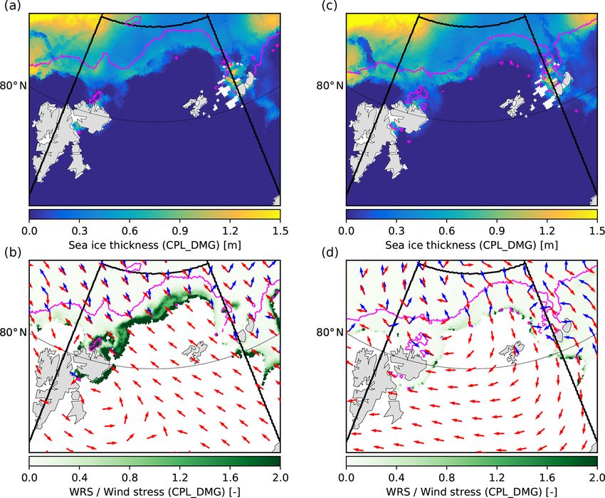
G. Boutin et al.: Wave–sea-ice interactions in a brittle rheological framework                                                   435

scaling laws of deformation in both time and space (Ram-            redistribution function associated with processes like frag-
pal et al., 2008; Marsan and Weiss, 2010). An ice cover such        mentation, lead opening, ridging and rafting. In our imple-
as the one illustrated in Fig. 2 is likely to have a very dif-      mentation, we assume that the only mechanical process mod-
ferent mechanical strength/response under external stresses         ifying the shape of the FSD is the wave-induced sea ice frag-
compared to a consolidated continuous ice cover due to the          mentation, and 8m is therefore the redistribution term asso-
high likelihood of break-up of the thin ice between the con-        ciated with this process. The advection terms for both FSDs
solidated floes. In the case of a new wave event, the fragmen-      are identical and similar to what is done for other conserva-
tation of the ice cover is likely to occur at its weakest points,   tive sea ice properties in neXtSIM. The terms 8th and 8m
i.e. at the thin ice joints. There have been very few reports       differ between gfast and gslow and are described below.
of sea ice break-up events in the literature (Liu and Mollo-
Christensen, 1988; Collins et al., 2015; Kohout et al., 2016),      2.2.1   Lateral sea ice melt/growth
but our intuition is supported by the recent Antarctic observa-
tions made by Kohout et al. (2016), who report waves break-         In this section, we describe the implementation of the terms
ing ice preferentially at refrozen cracks and pressure ridges.      8th,slow and 8th,fast that represent the thermodynamical re-
Introducing the slow-growth FSD in our model is therefore a         distribution of floes associated with lateral melt/growth in
way to keep a memory of the floe size resulting from the last       each FSD. The evolution of the FSD due to ice growth and
wave-induced fragmentation event in the model.                      melt processes is first performed in the fast-growth FSD, and
   These two FSDs are implemented in neXtSIM as areal               is quite similar to the implementation described by Roach
FSDs (as done by, e.g. Zhang et al., 2015; Roach et al., 2018;      et al. (2018):
Bateson et al., 2020; Boutin et al., 2020), which are defined       8th,fast =
as
                                                                               ∂gfast  2
D+dD
                                                                    − 2Gr −           + gfast + δ(D − DN )ċnew + βweld , (4)
 Z                                                                              ∂D     D
                         1
        g(D, x, t)dD =     aD (D, D + dD)                    (1)    where Gr is the lateral melt rate of floes, ċnew is the rate of
                         A
    D                                                               formation of new ice and βweld is the FSD redistribution term
                                                                    associated with welding of floes using the Smoluchowski
and
                                                                    equation as implemented by Roach et al. (2018).
Z∞                                                                     Lateral melting is implemented following Horvat and
  g(D, x, t)dD = 1.                                          (2)    Tziperman (2015) and Roach et al. (2018). Here, we neglect
0
                                                                    lateral melt for the largest floe size category as floes with size
                                                                    O(100) m and more are not resolved in this study and are ex-
   In these definitions, g(D) represents an FSD where D is its      pected to have very little contribution to lateral melt. We also
associated floe size, A is the total area considered around the     do not make any distinction between what they call the “lead
position x at a time t and aD are the areas within A covered        region” and the “open water fraction” of each grid cell, which
by sea ice with floes having diameters between D and D +            means the factor called φlead in Roach et al. (2018) is taken
dD. The value DR = 0 corresponds to open water and Eq. (2)          to be 1. Note that lateral melt is included in the model in this
                    ∞
is equivalent to 0+ g(D, x, t)dD = c, where c is the sea ice        study but is not discussed here, as we focus on the impact of
concentration. In practice, we have a number N of FSD bins          waves on sea ice dynamics during a time period dominated
of constant width 1D with edges between a minimum and               by freezing.
a maximum floe size, respectively, D0 and DN . Thus, floes             In contrast to Roach et al. (2018), sea ice is assumed to be
with sizes in [D0 D1 ] cannot be broken into smaller pieces,        unbroken when initialized in our model, and there is there-
and we refer to floes with sizes in [DN−1 DN ] as unbroken          fore no need for an explicit thermodynamical lateral growth
floes. Using fixed-width bins may bias our ability to represent     due to the agglomeration of frazil ice at the edge of existing
or examine scale-invariant behaviour (Stern et al., 2018), but      floes. If, after a wave-induced fragmentation event the sea
it has the advantage of being simple and the study of the FSD       ice concentration reaches 1 in freezing conditions, it is as-
evolution and its impact on sea ice is outside the scope of this    sumed that the newly formed sea ice is filling all leads, cre-
study.                                                              ating joints between the floes. The fast-growth FSD is there-
   Both FSDs evolve as in Roach et al. (2018) or Boutin et al.      fore redistributed so that all ice is considered to be made of
(2020):                                                             unbroken floes.
∂g(D)                                                                  The growth of small floes resulting from wave-induced
      = −∇ · (ug(D)) + 8th + 8m ,                            (3)    fragmentation in our model is also ensured by welding,
  ∂t
                                                                    which was shown by Roach et al. (2018) to generate a lat-
in which u corresponds to the sea ice velocity vector, 8th is       eral growth rate one order of magnitude higher than that aris-
a redistribution function of floe size due to thermodynamic         ing from the lateral accumulation of frazil ice. We, however,
processes (i.e. lateral growth/melt) and 8m is a mechanical         found the algorithm they used to be very dependent on the

https://doi.org/10.5194/tc-15-431-2021                                                       The Cryosphere, 15, 431–457, 2021
436                                                  G. Boutin et al.: Wave–sea-ice interactions in a brittle rheological framework

choice of the FSD categories. After some discussion with                   which we call λbreak , is passed to neXtSIM (see Fig. 1) and
the authors of Roach et al. (2018), we decided to carry on                 used in the mechanical redistribution scheme of the FSD. The
with this formulation but with an appropriate tuning of the                determination of the value of λbreak in WW3 was explained
coefficient that Roach et al. (2018) called κ, which repre-                in detail in Sect. 2.3 of Boutin et al. (2018) (where it is called
sents the rate at which the number of floes decreases due to               λi,break ). If no fragmentation has occurred in WW3, neXtSIM
welding per surface area. We tune κ so that the timescale at               receives λbreak = 1000 m, which corresponds to the default
which a delta-function FSD made of the smallest floes al-                  unbroken value, and no fragmentation occurs in neXtSIM
lowed in the model evolves into a delta-function FSD made                  (resulting in 8m,slow = 0 and 8m,fast = 0). If neXtSIM re-
of the biggest possible floes is similar in our model and in               ceives a value of λbreak < 1000 m, then FSD redistribution
the model by Roach et al. (2018). To give an idea of the                   occurs in neXtSIM. Fragmentation occurrence is then deter-
timescales involved, the model of Roach et al. (2018), start-              mined every coupling time step.
ing from a delta-function FSD only made of floes with an                      If fragmentation occurs, we assume that the thin ice join-
average size of 20 m, ends up with half the ice cover being                ing aggregated floes is very likely to break, as reported by
made of floes larger than 200 m in about 5 d within compact                Kohout et al. (2016). This is where the memory of previ-
sea ice (c = 0.95). In the simulations presented in this study,            ous cracks stored in the slow-growth FSD plays a role. In
setting κ = 5 × 10⁻⁸ m−2 s−1 reproduces a similar evolution                the model, the quick failure of the cementing thin ice is
of the FSD for our choice of FSD categories.                               represented by relaxing the fast-growth FSD, gfast , to the
   As mentioned earlier, the redistribution of the slow-growth             slow-growth FSD, gslow . In practice, we set 8m,thermo 1tice =
FSD due to lateral growth in 8th,slow is expected to happen                gfast − gslow , where 1tice is the ice model time step, therefore
on longer timescales that are related to the time needed by                assuming that this relaxation is almost instantaneous. We jus-
the fractures to heal. This healing phenomenon is related to               tify this short relaxation time by the fact that (i) waves can
the thickening and the consolidation of the joints, the forma-             fragment a consolidated sea ice cover in a few tens of min-
tion of which is described by 8th,fast . It is very similar to the         utes only (Collins et al., 2015) and (ii) the fast-growth FSD
“damage healing” already included in neXtSIM (see Rampal                   gfast is only used for thermodynamical processes associated
et al., 2016), and associated with a timescale τheal , that we             with timescales of at least a few hours and is therefore rela-
reuse in the computation of 8th,slow :                                     tively unaffected by the choice of a relaxation time value one
                                                                           order of magnitude lower.
              1                                                               Once fragmentation has occurred, the relaxation of the
8th,slow =           (gfast (Dfast ) − gslow (Dslow )) + 8conservation ,
             τheal                                                         fast-growth FSD to the slow-growth FSD gives gfast = gslow .
                                                                     (5)   This equality represents the fact that Dfast = Dslow when
where 8conservation is an ad hoc term ensuring the conserva-               fragmentation occurs and before thin ice starts cementing the
tion of sea ice area (i.e. Eq. 2) for the slow-growth FSD when             floes. In the model, the shape of the two FSDs after a frag-
sea ice is created or melted. The slow-growth FSD therefore                mentation event is then controlled by the mechanical redistri-
relaxes to the fast-growth FSD over a time τheal , represent-              bution occurring in the slow-growth FSD represented by the
ing the (slow) strengthening of the joints between the floes.              term 8m,slow . This term can be written in the same form as
Note that this healing only occurs if the sea ice is exposed to            in Zhang et al. (2015):
freezing conditions. If new sea ice is formed, all new ice is
added to the largest floe size category, as in the fast-growth             8m,slow =
FSD. If sea ice is melting, we assume that lateral melting has                              Z∞
little effect on the shape of the FSD. In this case, 8conservation         − Q(D)gslow (D) + Q(D 0 )β(D 0 , D)gslow (D 0 )dD 0 ,         (6)
is used to scale the slow-growth FSD without changing its
                                                                                                0+
shape.

2.2.2   Wave-induced sea ice fragmentation                                 where Q(D) is a redistribution probability function charac-
                                                                           terizing which proportion of floes of a given size D is bro-
In this section, we describe the implementation of the terms               ken (with D representing indistinctively Dfast and Dslow dur-
8m,slow and 8m,fast that represent the mechanical redistribu-              ing fragmentation) and β(D 0 , D) is a redistribution factor
tion of floes associated with the fragmentation of sea ice by              quantifying the fraction of sea ice concentration transferred
waves in each FSD.                                                         from floe size D 0 to D as fragmentation occurs. The choices
   Similar to the work by Boutin et al. (2020), the occur-                 of Q(D) and β(D 0 , D) therefore shape the FSD resulting
rence of sea ice fragmentation in our coupled system is de-                from wave-induced fragmentation. This shape is important
cided in the wave model. In WW3, sea ice breaks up if the                  as it strongly impacts processes involved in wave attenua-
wave curvature induces a stress that exceeds the sea ice flex-             tion (Boutin et al., 2018) and lateral melting (Bateson et al.,
ural strength. The shortest wavelength for which the wave-                 2020), but the evolution of the FSD during wave-induced
induced stress exceeds the critical stress for flexural failure,           fragmentation is still not well understood.

The Cryosphere, 15, 431–457, 2021                                                               https://doi.org/10.5194/tc-15-431-2021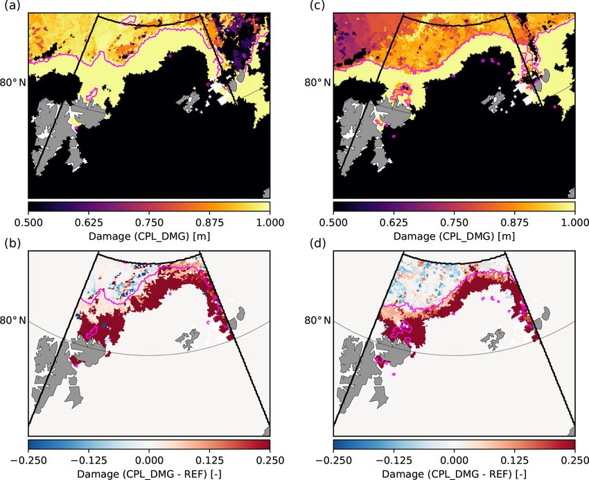
G. Boutin et al.: Wave–sea-ice interactions in a brittle rheological framework                                                  437

   Toyota et al. (2011) have suggested from field observa-          is computed as
tions that the shape of the FSDs could be interpreted as two                                 1/4
                                                                                 π 4 Y h3

truncated power laws separated by a cut-off floe size and                   1
                                                                    DFS =                         ,                             (7)
hypothesize that this cut-off corresponds to the critical floe              2 48ρg(1 − ν 2 )
size under which floes cannot be broken by waves. A cut-off
floe size also seems to be visible in the FSDs that Herman          where g is gravity, Y is the Young modulus of sea ice, ν is
et al. (2018) obtain from a laboratory experiment. The exis-        Poisson’s ratio, h is the mean sea ice thickness and ρ is the
tence of a cut-off floe size is, however, contested. The use        density of sea water. For ice thinner than 1 m, which is often
of cumulative distribution functions to interpret FSDs may          the case in the MIZ, DFS is lower than 15 m and the cut-off
give a false impression of scale invariance and the apparent        floe size is likely to be determined by the value of λbreak . To
change of regime could originate from finite measurement            define Q(D), we take an approach similar to Williams et al.
windows (Burroughs and Tebbens, 2001; Stern et al., 2018).          (2013b) and set
The division of the FSD into two truncated power laws sug-
                                                                               1
gested by Toyota et al. (2011) has nevertheless been used           Q(D) =         pFS (D, DFS )pλ (D, λbreak ),                (8)
to redistribute FSDs in the wave-in-ice models by Dumont                     τWF
et al. (2011) and Williams et al. (2013b), which have been          in which τWF is a relaxation time associated with wave-
reused for the wave-in-ice attenuation parameterization im-         induced fragmentation events, and pFS and pλ are probabil-
plemented in WW3 by Boutin et al. (2018) and in many other          ities that floes break depending on their size. We introduced
studies using wave-in-ice models (see, e.g. Aksenov et al.,         τWF to avoid dependency of the FSD redistribution to the
2017; Williams et al., 2017; Bennetts et al., 2017; Bateson         coupling time step. It represents the timescale needed for the
et al., 2020; Boutin et al., 2020).                                 FSD of a fragmenting sea ice cover to reach a new equilib-
   In this study, the FSD is mostly used to provide WW3 with        rium under a constant sea state. We set it to 30 min, as this
information on the floe size to estimate the wave attenuation.      corresponds to the timescale of the fragmentation event de-
The FSD does not impact the amount of new ice formed                scribed in Collins et al. (2015). The probability functions pFS
and we focus on periods during which lateral melting can            and pλ express the idea that the smaller the floes are, the less
be neglected. In these conditions it is advantageous to stay        chance they have to break. The function pλ compares the
close to what has been done already for the FSD in WW3              floe size D with the value of DFS and pλ compares the floe
in order to ensure that wave attenuation is not too different       size D with λbreak , introducing a dependency of Q(D) on the
from the one evaluated by Boutin et al. (2018) and Ardhuin          wave field. The difference with the model of Williams et al.
et al. (2018). We therefore build on the work by Zhang et al.       (2013b) is that instead of step functions we use hyperbolic
(2015) and Boutin et al. (2020) to suggest a new parameter-         tangents to get a continuous transition of Q(D) between 0
ization for Q(D) and β(D 0 , D) that redistributes the FSD in       and 1:
a similar way to the assumptions made in wave-in-ice mod-
els derived from Williams et al. (2013b). However, there are                                     D − c1,FS DFS
                                                                    pFS (D) = max 0, tanh                            ,          (9a)
two main differences from the FSDs assumed in Williams                                             c2,FS DFS
et al. (2013b): we allow the exponent of the power law cor-

                                                                                                       D − c1,λ λbreak
responding to the “small-floe” regime to vary and we smooth         pλ (D, λbreak ) = max 0, tanh                         ,    (9b)
                                                                                                         c2,λ λbreak
the transition between the small-floe regime and the “large-
floe” regime, as can be seen in the data from Toyota et al.         in which c1,FS , c2,FS , c1,λ and c2,λ are parameters of the
(2011).                                                             FSD that control the range of floe size that will be broken
   Q(D) represents the amount of ice in each floe size cat-         or not. The use of a continuous Q(D) instead of a step func-
egory that will be broken. Williams et al. (2013b) and a            tion aims to relax the constraint on the FSD shape imposed
number of further studies using their approach (Bennetts            by Williams et al. (2013b). With a step function, the prob-
et al., 2017; Bateson et al., 2020; Boutin et al., 2020) used a     ability of having floes larger than the cut-off floe size is 0,
step function with Q(D) = 1 if D ≥ 0.5λbreak and D ≥ DFS ,          i.e. above the cut-off floe size the FSD is suddenly infinitely
where DFS is the minimum floe size for which flexural fail-         steep. This approach is particularly problematic. First, the
ure can occur (see Mellor, 1986), and Q(D) = 0 if not. The          FSDs reported in Toyota et al. (2011) show a gradual steep-
transition of Q(D) from 0 to 1 occurs at a critical floe size un-   ening rather than a sharp transition. Second, the steepening
der which floes do not break, corresponding to what Toyota          of the FSD slope that led to the identification of the two floe
et al. (2011) interpreted as the cut-off floe size. In the model    size regimes by Toyota et al. (2011) could actually be due to
of Williams et al. (2013b), the transition therefore occurs at      windowing issues (Stern et al., 2018). Here, instead of hav-
max(DFS , 0.5λbreak ). DFS depends on sea ice properties and        ing a single cut-off floe size, we have a transition occurring
                                                                    in the floe size range for which 0 < Q(D) < 1. The width
                                                                    of this range is controlled by c2,FS and c2,λ . Q(D) tends to-
                                                                    wards a step function when c2,FS and c2,λ tend towards 0.

https://doi.org/10.5194/tc-15-431-2021                                                       The Cryosphere, 15, 431–457, 2021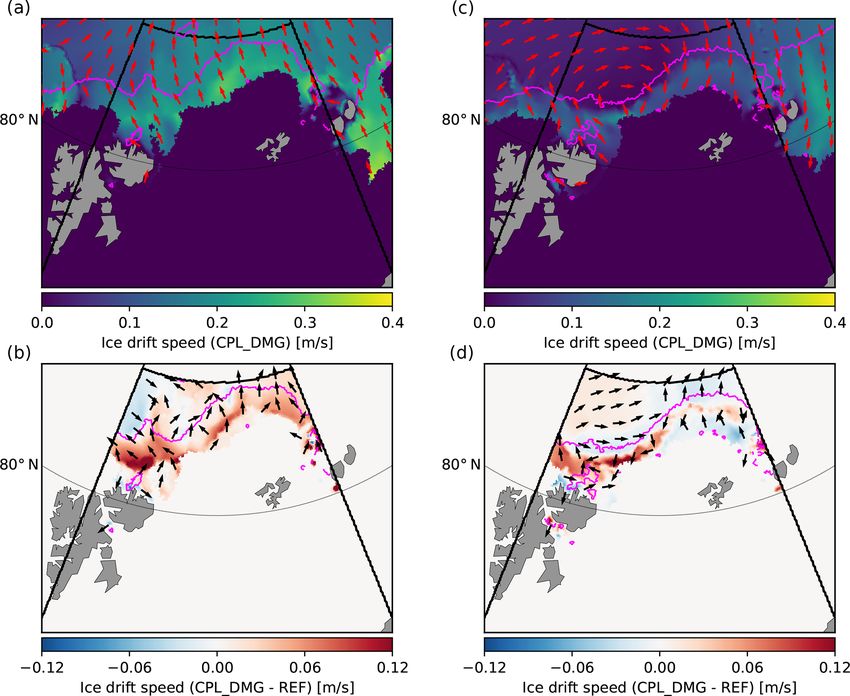
438 G. Boutin et al.: Wave–sea-ice interactions in a brittle rheological framework
We found that setting c2,FS = 2 and c2,λ = 2 leads to FSDs not prescribe a fixed value to the exponent α of this power
with a gradual steepening that look very similar to what is law. Instead, α decreases as the ice thickens and wavelength
reported by Toyota et al. (2011) or in the lab experiments increases as is shown and discussed in Sect. 4.1.2.
by Herman et al. (2018), for instance. The location of the The processes we use for the wave-in-ice attenuation com-
floe size range at which the transition occurs is controlled by putation in WW3 require the estimation of two floe size pa-
c1,FS and c1,λ . Like Williams et al. (2013b), we set c1,FS = 1. rameters: the average floe size hDi and the maximum floe
Instead of using c1,λ = 0.5 as in Williams et al. (2013b), we size Dmax (Boutin et al., 2018). When WW3 is run in stand-
set c1,λ = 0.3. It is consistent with the hypothesis made by alone mode, Dmax is taken to be λbreak /2 and an assump-
Boutin et al. (2018) that floes smaller than 0.3λbreak are tilted tion is made on the shape of the FSD after fragmentation al-
by waves but do not bend and therefore have no chance of lows us to estimate the value of hDi. When WW3 is coupled
suffering flexural failure. Reducing the value of c1,λ reduces with neXtSIM, the FSD is free to evolve to the sea ice model
the value of the cut-off floe size we should get, which gen- and it is necessary to estimate the value of Dmax and hDi in
erally leads to floes smaller than assumed in Williams et al. neXtSIM so it can be sent to WW3.
(2013b). It is, however, compensated for by using a contin- The average floe size hDi can be simply defined as
uous Q(D), which gives more weight to large floes than the
Z∞
FSD assumed in the model of Williams et al. (2013b). FSDs
generated by this redistribution function are presented and hDi = D g(D)dD. (12)
discussed in Sect. 4.1.2. 0
The redistribution factor β controls the shape of the FSD Here we use the slow-growth FSD, gslow (Dslow ), assum-
after it has been redistributed. Similar to the work by Zhang ing that wave scattering, which is the wave attenuation pro-
et al. (2015) and Boutin et al. (2020), the redistribution factor cess depending on hDi, is more affected by consolidated
β follows the form floes than by the thin ice joining them. The maximum floe
q q size, Dmax , definition is less straightforward, as it was origi-
β(Dn , D) = Dn − Dn−1 if Dn ≥ D
nally designed in the FSD parameterization of Dumont et al.
q
D q − D0 , (10)
(2011) to represent the largest floe size of a fragmented sea
β(Dn , D) = 0 otherwise ice cover, and if no fragmentation had occurred it was set to a
large default value. Here, this definition needs to be extended
where n corresponds to the index of the nth FSD category
to a coupled system with an FSD free to evolve under the
and q is an exponent that controls the shape of the redis-
effects of both mechanical and thermodynamical processes
tributed FSD. Zhang et al. (2015) used q = 1 arguing that
and able to represent a mix of fragmented floes and large ice
since the fragmentation of floes is a stochastic process, any
plates. We suggest a definition based on the percentage of
floe size lower than the initial unbroken floe can be generated
the ice cover area occupied by large floes, computing Dmax
with a similar probability. It leads to power-law FSDs after
as the 90th percentile of the areal FSD. Besides, the flexure
a succession of fragmentation events. Boutin et al. (2020)
dissipation mechanisms included in WW3 by Boutin et al.
noted that q is related to the (negative) exponent α of the
(2018) require us to discriminate between sea ice cover made
power-law FSD associated with the smaller floe sizes re-
of large floes with size on the order of O(100) m and an un-
sulting from the redistribution as assumed by Toyota et al.
broken sea ice cover for which the default Dmax in WW3
(2011) and later by Williams et al. (2013b) with q = 2 + α.
is set to 1000 m. This is because flexure only occurs if the
In their study, Toyota et al. (2011) related the exponent α to
wavelength is shorter or of the same order as the floe size.
a quantity they call fragility, which represents the probability
Knowing that long swells can have wavelengths on the order
of fragmentation of floes. Williams et al. (2013b) assumed
of O(100)m, they are only fully attenuated by inelastic dis-
that fragility is constant and equal to 0.9, giving α ' −1.85.
sipation if floe size is on the order of O(1000) m, which can
Boutin et al. (2020) set the value q to prescribe power-law
be larger than the floe size range covered by the FSD defined
FSDs with this same value of α but remain consistent with
in neXtSIM. In the case where DN < 1000 m, to make sure
what was done in wave models before. This is, however, a
that swells are still attenuated in an unbroken sea ice cover by
big constraint on the shape of the FSD, and it contradicts
WW3, we linearly increase the value of Dmax sent to WW3
the variations of the exponent of the power law fitted to the
from Dmax = DN to Dmax = 1000 m with R D the proportion of
small-floe regime reported by Toyota et al. (2011). Here, we
sea ice in the largest floe size category DNN−1 gslow (D)dD/c.
have already expressed the probability of fragmentation of
floes, hence the fragility, as the product of pFS and pλ . Using 2.3 Link between wave-induced sea ice fragmentation
this relationship, we get and damage
q = −log2 (pFS (D)pλ (D, λbreak )) . (11)
As mentioned in the Introduction, it is expected that sea ice
This definition of q still generates FSDs that tend to a power fragmentation by waves results in lowering the ice internal
law for floe sizes lower than the cut-off floe size, but it does stress. The lowering of sea ice resistance to deformation due
The Cryosphere, 15, 431–457, 2021 https://doi.org/10.5194/tc-15-431-2021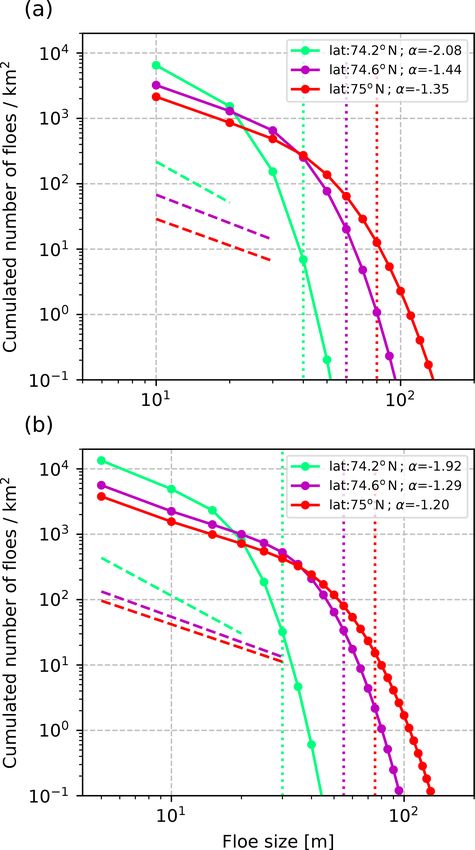
G. Boutin et al.: Wave–sea-ice interactions in a brittle rheological framework                                                  439

to a high density of cracks is already represented in neXtSIM      see Rampal et al. (2016). Wave–current interactions in WW3
by the variable called damage. This variable takes a value         are not considered in this study.
between 0 and 1, with 0 corresponding to undamaged sea                For the FSD in neXtSIM, we use 20 categories with a
ice, and 1 to a highly damaged sea ice cover, i.e. presenting      width 1D = 10 m. The lower bound D0 is set to 10 m, which
a high density of cracks. Sea ice damaging in neXtSIM is           is about the size of the smallest floes susceptible to undergo
usually due to the wind. In our study, we want it to have an       flexural failure (Mellor, 1986). The upper bound of the FSD,
additional dependence on wave-induced sea ice fragmenta-           DN , is therefore equal to 210 m, which is on the order of
tion. In our implementation, it is possible to quantify the sea    magnitude of the largest floes resulting from wave-induced
ice cover area that is susceptible to being broken by waves        sea ice fragmentation generated by WW3. The healing relax-
if WW3 provides a value of λbreak < 1000 m as cbroken =           ation time τheal used by neXtSIM is set to its default value of
c 1 − e−1tcpl /τWF and cbroken = 0 if λbreak ≥ 1000 m. As the      25 d (Rampal et al., 2016).
fragmentation of sea ice by waves can break ice plates into
floes with sizes up to a few hundred metres and the horizontal     3.2   Evaluation of the FSD implementation: model
resolution of the model mesh is in general at least a few kilo-          set-up
metres, we hypothesize that areas of the sea ice cover frag-
mented by waves are associated with high values of damage,         In Sect. 4.1, we use sea state and sea ice observations made in
i.e. close to 1. We thus suggest computing the new damage          the Beaufort Sea in the framework of the Arctic Sea State and
value associating a value of dw = 0.99 to cbroken , which gives    Boundary Layer Physics Program (Thomson et al., 2018) to
the following evolution of the damage d:                           evaluate the wave attenuation and broken sea ice extent in our
                                                                   coupled simulations, which is similar to what Ardhuin et al.
d = min (1, d(1 − cbroken ) + dw cbroken ) .               (13)    (2018) did with stand-alone WW3 simulations. To do so, we
                                                                   ran five simulations from 10–13 October 2015, a period cov-
This process is repeated every time fragmentation occurs in        ering the storm event investigated in a study by Ardhuin et al.
the sea ice model. Note that because wave events generally         (2018). This storm generated ' 4 m waves fragmenting the
last for a few hours, this damaging process is generally re-       sea ice edge in the Beaufort Sea from 11–12 October 2015.
peated enough times to result in little sensitivity of the model      The first of these simulations was a WW3 uncoupled sim-
to values of dw between 0.1 and 1. Note also that floe size and    ulation hereafter labelled ARD18, as it used the exact same
damage are not explicitly linked by this relationship, but the     parameterization as the one labelled REF2 in Ardhuin et al.
relaxation time associated with the healing of damage and          (2018). The only difference is that here it was run on the
the slow-growth FSD are the same, making their evolution           CREG025 grid used for all our simulations. This parame-
parallel in the regions of broken ice.                             terization of the wave model was chosen as it showed the
                                                                   best match with observations for both wave height and bro-
3     Model set-up                                                 ken sea ice extent in the study by Ardhuin et al. (2018).
                                                                   We also used the same sea ice concentration data as Ard-
3.1    General description of the pan-Arctic configuration         huin et al. (2018) to force the uncoupled wave model. They
                                                                   were obtained from a re-analysis of the 3 km resolution sea
Similarly to Boutin et al. (2020), the coupled framework           ice concentration dataset derived from the AMRS2 radiome-
is run on a regional 0.25◦ grid (CREG025), which covers            ter using the ASI algorithm (Kaleschke et al., 2001; Spreen
the Arctic Ocean at an approximate resolution of 12 km as          et al., 2008)1 . This re-analysis produced 12-hourly maps that
well as some of the North Atlantic. As neXtSIM is a finite-        gathered all the AMSR2 passes acquired between 00:00 and
element sea ice model using a moving Lagrangian mesh, it           13:59 UTC and 10:00 and 23:59 UTC for the morning (AM)
is not run on a grid. Its initial mesh is, however, based on a     and evening (PM) fields, respectively. Similarly to Ardhuin
triangulation of the CREG025 grid, giving a prescribed mean        et al. (2018), sea ice thickness was set constant to 15 cm. Sea
resolution (i.e. mean length of the edges of the triangular ele-   ice concentration was also kept constant to make the compar-
ments) of 12 km. In coupled mode, neXtSIM interpolates the         ison with a coupled simulation easier. Sea ice concentration
fields to be exchanged onto the fixed grid so that the coupler,    for this 3 d run corresponded to the conditions on the evening
OASIS, is only required to send and receive different fields       of 12 October provided by the AMSR-2 sea ice concentration
(i.e. OASIS does not need to do any interpolation).                re-analysis at the same time as illustrated in Ardhuin et al.
   neXtSIM is run with a time step of 20 s, and WW3 with a         (2018) study. Initial wave conditions were provided by an
time step of 800 s. Fields between the two models are ex-          initial 10 d run of this simulation, from 1–10 October 2015,
changed every 2400 s. Atmospheric forcings are provided            in which sea ice concentration is updated every 12 h.
by 6-hourly fields from the CFSv2 atmospheric re-analysis
(Saha et al., 2014). In addition, neXtSIM is also forced by          1 AMSR2 data are available at https://seaice.uni-bremen.de/data/
ocean fields from the TOPAZ4 re-analysis (Sakov et al.,            amsr2/asi_daygrid_swath/n3125/2015/oct/Arctic3125/ (last access:
2012). For more details on the forcings used by neXtSIM,           November 2020).

https://doi.org/10.5194/tc-15-431-2021                                                      The Cryosphere, 15, 431–457, 2021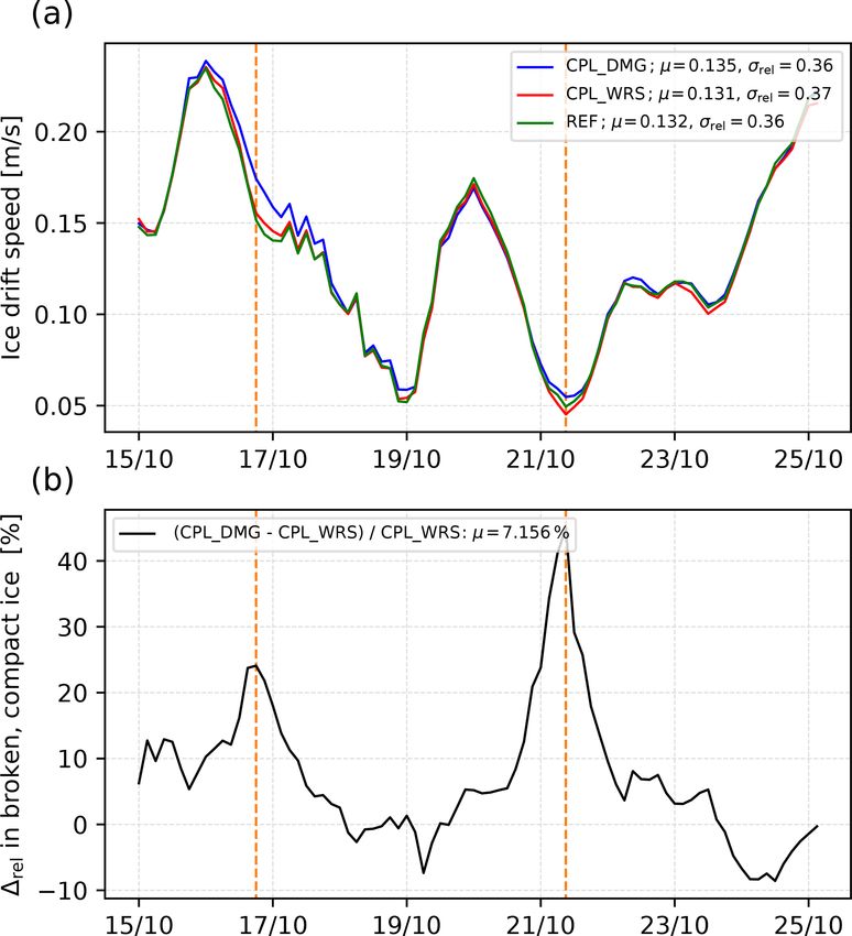
440                                          G. Boutin et al.: Wave–sea-ice interactions in a brittle rheological framework

   Secondly, we ran a coupled neXtSIM–WW3 simulation              4     Results
(hereafter labelled NXM/WW3). Initial conditions were the
same as in ARD18. Sea ice dynamics and thermodynam-               4.1     Evaluation of wave–sea-ice interactions in the
ics were switched off in neXtSIM so that we can compare                   coupled framework
the two simulations with a similar constant sea ice cover
(thickness and concentration). The only difference between        We first evaluate the representation of wave–ice interactions
ARD18 and NXM/WW3 was the way the evolution of floe               in our coupled framework. As our goal is to investigate the
size was treated, which is what we wanted to evaluate.            potential impact of waves on sea ice dynamics, we must en-
   Then, to illustrate the sensitivity of our results to the      sure that the coupled framework produces a consistent wave-
sea ice thickness value, we re-ran ARD18 and NXM/WW3              in-ice attenuation, as it is directly proportional to the WRS,
while this time setting the sea ice thickness to 30 cm. We        as well as reasonable extents of broken sea ice and timescales
named these two additional simulations ARD18_H30 and              of the ice recovery from fragmentation. In the following, we
NXM/WW3_H30, respectively.                                        consider the wave attenuation and extent of fragmented sea
   Finally, to investigate the sensitivity of the FSD evolution   ice on one hand, and the evolution of the FSDs after frag-
to the floe size categories used for the FSD, we ran a sim-       mentation events on the other hand.
ulation similar to NXM/WW3 but with a refined FSD that
we call NXM/WW3_refine. For this simulation, the num-             4.1.1    Evaluation of wave attenuation and extent of
ber N of categories was set to 41 instead of 20 and we set                 fragmented sea ice
1D = 5 m and D0 = 5 m. We also evaluated the evolution of
the two FSDs with refreezing/healing using the CPL_DMG            To evaluate the capacity of our coupled framework to pro-
simulation described in Sect. 3.3.                                duce reasonable wave-in-ice attenuation and extent of broken
                                                                  sea ice, we focused on the same event used to evaluate the
                                                                  WW3 parameterization of Boutin et al. (2018) in the study
3.3   Estimation of the impact of wave-induced
                                                                  by Ardhuin et al. (2018). Here, we used the ARD18 sim-
      fragmentation on sea ice dynamics: model set-up
                                                                  ulation as a reference, as it was shown to match well with
                                                                  observations for both the extent of broken ice and the wave
In Sect. 4.2, we compare the results of three simulations in      attenuation in this particular case. The comparison was done
order to investigate the wave impact on sea ice dynamics in       on 12 October at 17:00 GMT (Fig. 3). We also compared our
the MIZ. The first one (called REF) is a stand-alone simula-      model results with estimated wave height from SAR images
tion of neXtSIM. The second one (CPL_WRS) includes all            (Stopa et al., 2018a) and buoy measurements (AWAC, see
the features presented in Sect. 2 but uses the relationship be-   Thomson et al., 2018) along a transect in Fig. 3d.
tween wave-induced sea ice fragmentation and damage pre-             We evaluated the wave attenuation by looking at the evo-
sented in Sect. 2.3. The third simulation (CPL_DMG) is sim-       lution of the maximum floe size Dmax and significant wave
ilar to CPL_WRS except that it also includes a link between       height in the ice. Overall, the spatial distribution of these
the damage variable d and wave-induced sea ice fragmen-           two quantities in ARD18 and NXM/WW3 was very sim-
tation as described in Sect. 2.3. These simulations were run      ilar and also very similar to the results of Ardhuin et al.
from 15 September to 1 November 2015. This period was             (2018) (see Fig. 9 of their study). Figure 3d shows the wave
selected because refreezing occurs in the MIZ, meaning that       height evolution along a transect following the footprint of
the differences between REF and the two coupled simula-           Sentinel 1-a; again, we see almost no difference between
tions were not due to the change in lateral melting param-        ARD18 and NXM/WW3. Both simulations showed reason-
eterization. This period of the year is also characterized by     able agreement with the wave heights estimated from SAR
the combination of a low sea ice extent (thus a large avail-      and from the AWAC buoy. Similar to the results of Ardhuin
able fetch) and regular occurrence of storms in the Arctic,       et al. (2018), the model, however, seemed to slightly over-
which increases the opportunities to evaluate the impact of       estimate the wave height within the ice cover. This overesti-
waves on sea ice with fragmentation events over wide ar-          mation could have resulted from the assumption of constant
eas. The level of damage in the ice cover was initially set       thickness and low value (15 cm). This is visible in Fig. 3d
to zero where sea ice is present. Initial sea ice concentration   where most observations actually show higher significant
and thickness were set from the TOPAZ4 re-analysis (Sakov         wave height values than the one yielded by ARD18_H30 and
et al., 2012) and sea ice is unbroken. The wave field in WW3      NXM/WW3_H30, which use a constant thickness of 30 cm.
was initially at rest. The wave-in-ice attenuation parameteri-       Sea ice break-up occurrence depending on wave proper-
zation in WW3 in CPL_WRS and CPL_DMG was the same                 ties, comparable wave attenuation in between ARD18 and
as in ARD18 (i.e. REF2 in Ardhuin et al., 2018). We inves-        NXM/WW3 resulted in little difference in the extent of bro-
tigated the results of these simulations from 1 October, thus     ken sea ice between the two simulations (Fig. 3a, c). Al-
allowing for 16 d of spin-up, which is enough for the wave        though the extent of broken ice was slightly smaller in the
and damage fields to develop.                                     coupled run, the difference did not exceed two grid cells and

The Cryosphere, 15, 431–457, 2021                                                      https://doi.org/10.5194/tc-15-431-2021
G. Boutin et al.: Wave–sea-ice interactions in a brittle rheological framework 441
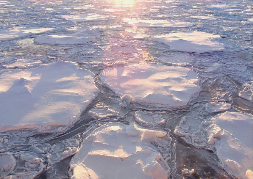
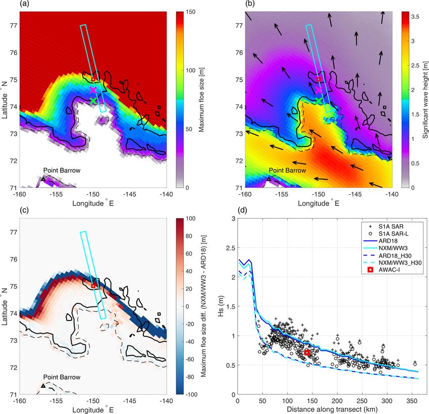
Figure 3. Spatial distributions of maximum floe size (a) and significant wave height (b) in the Beaufort Sea taken from the NXM/WW3
simulation on 12 October at 17:00:00 GMT. Black arrows indicate the wave mean direction. The difference of the maximum floe size
distribution with the ARD18 simulation is shown in panel (c). Evolution of the significant wave height for different simulations along the
transect depicted in cyan in panels (a)–(c) is presented in panel (d), along with significant wave height estimated from Sentinel-1a SAR
images (see Stopa et al., 2018a; Ardhuin et al., 2018, for details) and measured by an AWAC buoy. The AWAC position is depicted by a red
square in panels (a)–(c). The green and magenta crosses indicate the position at which the FSDs are shown in Fig. 4. Solid and dashed black
lines represent contours of sea ice concentration equal to 0.8 and 0.15, respectively. Point Barrow is indicated by a black triangle.
therefore represented a distance of about 25 km, which is ac- induced sea ice fragmentation occurs. This section provides
ceptable given the large uncertainties associated with wave a brief evaluation of these new features.
attenuation in ice (see, for instance, Nose et al., 2020). More- We first look at the FSD resulting from wave-induced frag-
over, as in Ardhuin et al. (2018), the broken sea ice region ex- mentation in neXtSIM by plotting the cumulative distribu-
tended up to about 15 km in-ice beyond the AWAC buoy (red tion of floes (CDF; see, e.g. Toyota et al., 2011; Herman
square), which matched well with the SAR images observed et al., 2018) for three different locations (Fig. 4) for the
for that same day. NXM/WW3 and NXM/WW3_refine simulations. Note that
because thermodynamical and dynamical processes are un-
4.1.2 Evaluation of the evolution of the FSDs activated in NXM/WW3, the fast- and slow-growth FSDs are
identical. The CDFs look very similar to the one reported by,
e.g. Toyota et al. (2011), with the curve gradually steepening
Our coupled framework introduces two FSDs to represent the as floe size increases. Following the method of Toyota et al.
evolution of the floe size from two different points of view. It (2011), two lines can be fitted to the FSD for small and large
also introduces a new redistribution scheme used when wave-
https://doi.org/10.5194/tc-15-431-2021 The Cryosphere, 15, 431–457, 2021You can also read