The behavioral impact of catch-and-release angling assessed through high resolution biotelemetry in the wild in two model freshwater species ...
←
→
Page content transcription
If your browser does not render page correctly, please read the page content below
H UMBOLDT U NIVERSITÄT ZU B ERLIN

           FACULTY OF L IFE S CIENCES
D ANIEL T HAER -I NSTITUTE OF A GRICULTURAL AND
           H ORTICULTURAL S CIENCES

                        M ASTER T HESIS

The behavioral impact of catch-and-release
 angling assessed through high resolution
  biotelemetry in the wild in two model
            freshwater species
    Author:                                                 Supervisors:
    Maximilian Rieble                      Prof. Dr. Robert Arlinghaus
                                                  Christopher T. Monk

           A thesis submitted in fulfillment of the requirements
         for the degree of Master of Sciencein the study program:
                  Fish Biology, Fisheries and Aquaculture
                                  in the

                             IFishman Lab
     Leibniz-Institute of Freshwater Ecology and Inland Fisheries

                            January 4, 2021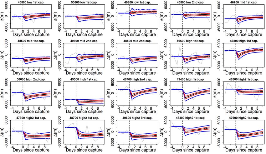
Statutory Declaration

I, Maximilian Rieble, declare that this thesis, titled "The behavioral impact of catch-
and-release angling assessed through high resolution biotelemetry in the wild in two
model freshwater species" and the work presented in it are my own. I confirm that:

   • This work was done wholly or mainly while in candidature for a research degree
        at this University.

   • Where any part of this thesis has previously been submitted for a degree or
        any other qualification at this University or any other institution, this has been
        clearly stated.

   • Where I have consulted the published work of others, this is always clearly at-
        tributed.

   • Where I have quoted from the work of others, the source is always given. With
        the exception of such quotations, this thesis is entirely my own work.

   • I have acknowledged all main sources of help.

   • Where the thesis is based on work done by myself jointly with others, I have
        made clear exactly what was done by others and what I have contributed myself.

Signed:

Date:

                                             I
Abstract

Catch-and-release (CR) angling is a widespread practice, but there is no scientific con-
sensus about its consequences on fish behaviour or mortality. Many studies on CR
impacts were conducted in laboratory or other artificial settings, which may inflate
CR impacts relative to studies in the wild. Species-specific investigations in situ are
necessary to understand how to minimise potential adverse effects of CR. I studied
the lethal and sublethal effects of CR angling in common carp (Cyprinus carpio; n =
43) and Eurasian perch (Perca fluviatilis; n = 36) in the wild. Carp and perch were re-
leased with acoustic transmitters into a shallow lake and equipped with a whole-lake
high-resolution acoustic telemetry system. After a four-week recovery phase 9 carp
and 14 perch were caught and-released at least once, monitored for six months and
compared to uncaptured controls. I hypothesised that (1) directly after a CR event, re-
ductions in relative swimming activity will occur, (2) that those changes would recover
to pre-capture levels within several days, (3) that CR impacts would vary within and
between species, (4) that CR events would increase the mortality risk of fish but only
to a small degree given the shallow study lake, precluding barotrauma, and finally,
(5) that responses to CR would be moderated by environmental effects such as water
temperature and oxygen during capture and to some extent by fish total length. To
investigate the behavioural impacts, I developed a novel method by modifying pro-
gressive change Before-After Change-Impact Paired-Series (BACIPS) analysis. Pro-
longed changes in activity for both carp and perch, on average ten and seven days
respectively, in response to CR were detected, longer than previously documented.
The most active fish showed the sharpest post-release activity decline and the longest
recovery. Cluster analyses revealed high within-species variation in impact, from low
to potentially severe. Behavioural impact severity in perch, but not carp, was driven
by environmental factors during the CR event. I found no evidence for lethal effects of
CR in carp or perch. Overall, my findings suggest that mortality from perch and carp
angling is negligible in shallow lakes. Further, mortality should not be the only indica-

                                           II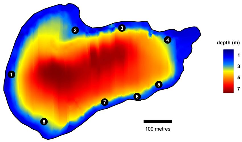
tor of CR impacts as species that are resilient to CR mortality might show prolonged
behavioural responses. Yet, these responses are not uniform across the population
and vary with the behavioural type and with the environment. Guidelines should be
adapted to minimize targeting highly active fish, which are both more likely to get
captured and to suffer adverse effects from CR angling.

                                         III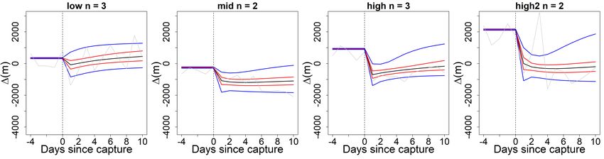
Acknowledgement

I am very grateful to Prof. Dr. Robert Arlinghaus for the opportunity to work on
this interesting project, as well as the patience and guidance I was afforded during the
writing of this work. Many thanks also to Christopher T. Monk, who was a great advi-
sor and an incredibly helpful source of feedback throughout the writing of this work,
and who further helped me to understand how the data in this study was acquired.
I want to further thank Prof. Dr. Robert Ahrens (NOAA) for his advice in develop-
ing the impact function, and Andrea Campos Candela for her help in modifying the
progressive-change BACIPS model and for her advice on bayesian modelling. Further
I am grateful to all the anglers and volunteer scientists involved in gathering the data
for this study in the field.

                                          IV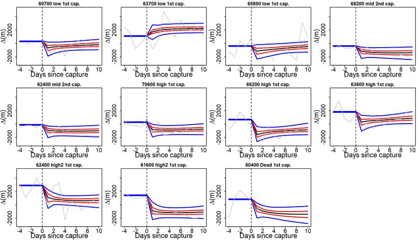
Contents

Statutory Declaration                                                                          I

Abstract                                                                                      II

Acknowledgement                                                                              IV

1   Introduction                                                                              1

2   Material and Methods                                                                      6
    2.1   Methods Overview . . . . . . . . . . . . . . . . . . . . . . . . . . . . . . .      6
    2.2   Study Species and Study Site . . . . . . . . . . . . . . . . . . . . . . . . .      6
    2.3   Fish Sampling and Tagging . . . . . . . . . . . . . . . . . . . . . . . . . .       9
    2.4   Experimental Angling . . . . . . . . . . . . . . . . . . . . . . . . . . . . . 10
    2.5   Swimming Distance Calculation . . . . . . . . . . . . . . . . . . . . . . . 13
    2.6   Mortality Assessment . . . . . . . . . . . . . . . . . . . . . . . . . . . . . . 13
    2.7   Statistical Analysis . . . . . . . . . . . . . . . . . . . . . . . . . . . . . . . 13
          2.7.1   Impact Assessment . . . . . . . . . . . . . . . . . . . . . . . . . . . 17
          2.7.2   Cluster Analysis . . . . . . . . . . . . . . . . . . . . . . . . . . . . 17
          2.7.3   Environmental Correlates of Catch-and-Release Response . . . . 18

3   Results                                                                                  19
    3.1   Descriptive Behaviours of Target Species . . . . . . . . . . . . . . . . . . . 19
    3.2   Experimental Catch-and-Release Angling . . . . . . . . . . . . . . . . . . 20
    3.3   Mortality . . . . . . . . . . . . . . . . . . . . . . . . . . . . . . . . . . . . . 20
    3.4   Model Results . . . . . . . . . . . . . . . . . . . . . . . . . . . . . . . . . . 22
    3.5   Cluster Analysis . . . . . . . . . . . . . . . . . . . . . . . . . . . . . . . . . 23
    3.6   Environmental Correlates of Catch-and-Release Response . . . . . . . . 26

4   Discussion                                                                               30
    4.1   Effects of Catch-and-Release on Swimming Activity . . . . . . . . . . . . 31

                                               V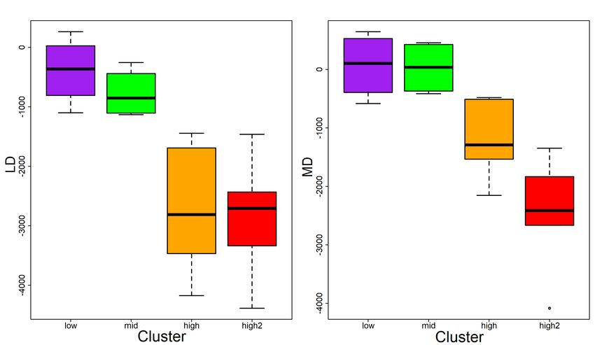
4.2   Effects of Catch-and-Release Angling on Mortality . . . . . . . . . . . . . 35
  4.3   Environmental Correlates of Catch-and-Release Response . . . . . . . . 36
  4.4   Modified Progressive-Change BACIPS approach . . . . . . . . . . . . . . 37
  4.5   Study limitations and future research . . . . . . . . . . . . . . . . . . . . . 38
  4.6   Conclusions . . . . . . . . . . . . . . . . . . . . . . . . . . . . . . . . . . . 39

A R code                                                                                     II
  A.1 Calculation of daily swimming distances and delta time series around
        catch events . . . . . . . . . . . . . . . . . . . . . . . . . . . . . . . . . . .   II
  A.2 Modified progressive change BACIPS . . . . . . . . . . . . . . . . . . . . IV

                                             VI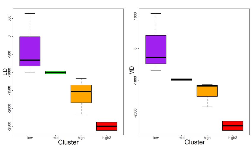
List of Figures
2.1 Map of study lake with hydrophone positions marked in black, pro-
vided by David March (IGB) . . . . . . . . . . . . . . . . . . . . . . . . . . 7
2.2 Depth Map of Kleiner Döllnsee with feeding site locations, Sites 2,4,6
and 8 were used as angling sites. (from Monk and Arlinghaus 2017) . . . 12
2.3 Example of mortality assessment data showing all calculated daily po-
sitions of a perch in this study on two days, plotted over the shoreline
of the study lake. Picture on the left shows movement of a living perch,
picture on the right shows a stationary signal in a case where mortality
was ascribed. . . . . . . . . . . . . . . . . . . . . . . . . . . . . . . . . . . 14
2.4 Step 1: Selecting daily swimming activity estimates around CR event
for impacted fish (red) and fish in control group (black). Step 2: Cal-
culate mean of control group. Step 3: Calculate difference between Im-
pacted Fish and Control Group (∆) . . . . . . . . . . . . . . . . . . . . . . 16
3.1 Mean daily swimming activity estimates in metres per day for (A) carp,
between December 6, 2014 and June 30, 2015, and (B) perch, between
October 29, 2014 and March 31, 2016. Experimental angling phases
marked in red, the black lines were fit to the mean daily activity esti-
mates of all tagged fish of the species (black points). . . . . . . . . . . . . 19
3.2 Mortality assessment of Carp ID 62400, sequence of daily positions shown
inside the shoreline of Kleiner Döllnsee. CR events marked in orange,
date of mortality marked in red. . . . . . . . . . . . . . . . . . . . . . . . . 21
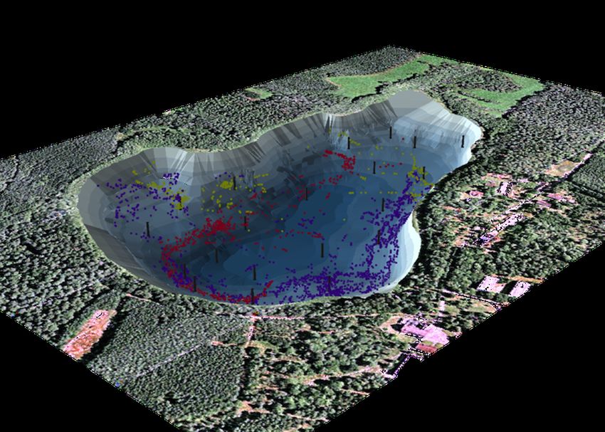
3.3 Credible intervals (CI) of individual perch impact model fits (95% CI in
blue, 50% CI in red, mean prediction in black) with relative swimming
activity estimates (grey line), sorted by impact type. The dashed vertical
line marks the moment of capture whereas the numbers on the y-axis
marks the number of days from capture . . . . . . . . . . . . . . . . . . . 22
VII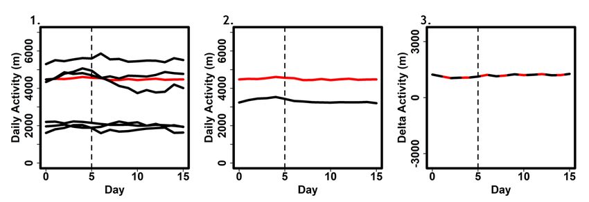
3.4   Credible intervals (CI) of individual perch impact model fits (95% CI
      in blue, 50% CI in red, mean prediction in black) with relative activity
      estimates (grey line), sorted by impact type. The dashed vertical line
      marks the moment of capture whereas the numbers on the y-axis marks
      number of days from capture . . . . . . . . . . . . . . . . . . . . . . . . . 23
3.5   Population level model predictions of (A) carp and (B) perch ∆ in metres
      per day with credible intervals (CI) (95% CI: blue lines, 50% CI: red
      lines, mean prediction: black line). The grey line denotes the observed
      mean ∆ and the vertical dashed line marks the moment of capture. . . . 24
3.6   Dendrograms of hierarchical clustering analysis using randomForest al-
      gorithm for carp (left) and perch (right) . . . . . . . . . . . . . . . . . . . 24
3.7   Range of mean difference (MD) and largest difference (LD) within carp
      impact clusters. Cluster sizes: . . . . . . . . . . . . . . . . . . . . . . . . . 25
3.8   Mean impact model predictions of relative carp swimming activity, in
      metres per day, by cluster. Sorted by impact severity (from left to right:
      low, medium, high1, high2) with credible intervals (CI) (95% CI: blue
      lines, 50% CI: red lines, mean prediction: black line). The grey line
      denotes the observed mean ∆ and the vertical dashed line marks the
      moment of capture. . . . . . . . . . . . . . . . . . . . . . . . . . . . . . . . 26
3.9   Mean impact model predictions of relative perch swimming activity, in
      metres per day, by cluster. Sorted by impact severity from left to right:
      low, medium, high1, high2. with credible intervals (CI) (95% CI: blue
      lines, 50% CI: red lines, mean prediction: black line). The grey line
      denotes the observed mean ∆ and the vertical dashed line marks the
      moment of capture. . . . . . . . . . . . . . . . . . . . . . . . . . . . . . . . 27
3.10 Range of Mean difference (MD) and largest difference (LD) by perch
      impact cluster. . . . . . . . . . . . . . . . . . . . . . . . . . . . . . . . . . . 27

                                         VIII
List of Tables
2.1 Overview of all tagged carp and perch remaining by the beginning of
experimental catch-and-release angling. IGB: Leibniz-Institute of Fresh-
water Ecology and Inland Fisheries. . . . . . . . . . . . . . . . . . . . . . 11
3.1 Candidate model set for generalised linear models predicting mortal-
ity using both impact and control group fish per species. CatchNr =
Number of captures, zero for control group. Best performing models in
bold. . . . . . . . . . . . . . . . . . . . . . . . . . . . . . . . . . . . . . . . 21
3.2 Impact cluster overview, cluster size pre-capture delta, largest post-
release difference (LD) and mean post-release difference (MD) relative
swimming activity in metres per day . . . . . . . . . . . . . . . . . . . . 27
3.3 Results of Generalised Linear Model predicting mean difference (MD)
in relative swimming activity following carp captures (N = 11). TL =
fish total length; ODO = dissolved oxygen content. . . . . . . . . . . . . . 28
3.4 Results of Generalised Linear Model (GLM) predicting largest differ-
ence (LD) in relative swimming activity following carp captures (N =
11). TL = fish total length; ODO = dissolved oxygen content. . . . . . . . 28
3.5 Multinomial log-linear model results for carp; Estimate (sd), p-value
of effects on ranked impact types (low, mid, high1, high2) by fish total
length (TL), temperature, and oxygen saturation of the water during
capture. . . . . . . . . . . . . . . . . . . . . . . . . . . . . . . . . . . . . . . 28
3.6 Results of Generalised Linear Model predicting mean difference (MD)
in relative swimming activity following perch captures (N = 20). TL =
fish total length; ODO = dissolved oxygen content. . . . . . . . . . . . . . 29
3.7 Results of Generalised Linear Model predicting largest difference (LD)
in relative swimming activity following perch captures (N = 20). TL =
fish total length; ODO = dissolved oxygen content. . . . . . . . . . . . . . 29
IX3.8 Multinomial log-linear model results for perch; Estimate(sd), p-value
of effects on ranked impact types (low, mid, high1, high2) by fish to-
tal length (TL), temperature, turbidity, and dissolved oxygen saturation
(ODO) of the water during capture. . . . . . . . . . . . . . . . . . . . . . . 29
XChapter 1
Introduction
Catch-and-release (CR) angling is the practice of unhooking fish caught by hook and
line angling and releasing the living fish back into the water. It is a byproduct of har-
vest regulations like bag limits (e.g. maximum number of caught fish) and size limits
(e.g. maximum and/or minimum size for harvestable fish) (Arlinghaus, Cooke, et al.
2007). In Western industrialised countries, where most recreational fisheries are man-
aged using variations of length-based regulations (Arlinghaus, Mehner, and Cowx
2002), CR is a common occurrence. Moreover, many anglers engage in voluntary CR
(Arlinghaus, Cooke, et al. 2007). Depending on culture, CR angling is considered ei-
ther as contributing to conservation (Cooke and Philipp 2004, Cooke and Suski 2005;
Cooke, Donaldson, et al. 2013) or as a reprehensible practice by anglers that is deeply
unethical (Arlinghaus, Schwab, et al. 2012). For example, anglers in Germany risk
prosecution under the Animal Protection Act ("Tierschutzgesetz") (Arlinghaus, Cooke,
et al. 2007) when voluntarily releasing harvestable fish, as fishing for food is regarded
as the sole legitimate motivation for harming animals. Given the common occurrence
of CR and despite the controversy around CR, it is important to know what happens
iologically to a fish and whether the released fish is affected through a pervasive stress
response (Jendrusch and Arlinghaus 2005).
Mortality rates induced by CR are non-zero and can be substantial under certain
ecological conditions and for certain species (Hühn and Arlinghaus 2011; Bartholomew
and Bohnsack 2005; Muoneke and Childress 1994). When hooking mortalities ex-
ceed ∼ 25% (Johnston, Beardmore, and Arlinghaus 2015), the implementation of size-
specific regulations can fail to curtail recruitment overfishing (Coggins et al. 2007, Pine
et al. 2008). In a meta-analysis by Bartholomew and Bohnsack (2005) on the factors in-
fluencing mortality in the context of CR, hooking location was identified as the most
important factor for within species variation in hooking mortality. Other factors re-
1lated to the angling event include hooking depth, angling gear, angler skill, as well as
playing and handling times (Muoneke and Childress 1994; Bartholomew and Bohn-
sack 2005). The outcome of CR angling also depends on intrinsic characteristics of the
fish like age, condition, size or previous exposure to stress, and further on environ-
mental conditions during capture such as temperature, dissolved oxygen, or depth
(biotic factors) and disease or predator burden (abiotic factors) (Arlinghaus, Cooke,
et al. 2007). The depth from which a fish is caught affects the risk of barotrauma, and
there is a risk for post-release predation when fish are angled to exhaustion or substan-
tially injured during CR (Bartholomew and Bohnsack 2005). Among the environmen-
tal factors, water temperature has been identified as an important factor, and to a lesser
extent dissolved oxygen content (ODO) of the water (Cooke and Suski 2005). The use
of CR angling as a conservatory management tool depends on high survival rates fol-
lowing CR (Muoneke and Childress 1994). Surviving CR angling does not, however,
mean that a fish is not impacted from the CR event, as lasting sublethal effects on
the physiology and behaviour of caught-and-released fish are possible (Arlinghaus,
Laskowski, et al. 2017). Studying mortality effects and behavioural responses of fish
associated with CR is one way to understand the impact that angling induces on them.
The response of fish towards significantly stressful events happens on multiple
levels (Bonga 1997). The primary response takes place in the neuro-endocrine sys-
tem (e.g. increased adrenaline levels), followed by a secondary stress response in the
blood and muscle tissues (e.g. release of glucose, increased heart rate and blood pres-
sure) (Arlinghaus, Cooke, et al. 2007; Schreck, Olla, and Davis 1997). This may in turn
elicit a tertiary stress response in the form of whole-fish changes in performance such
as reduced growth, disease resistance as well as changes in behaviour (Bonga 1997).
Therefore, when studying responses to stressors, behavioural responses may serve as
an integrative measure of high validity (Iwama, Afonso, and Vijayan 1998). While the
primary and secondary stress responses are comparatively easy to measure and ob-
serve in laboratory conditions, the tertiary stress response is embedded in and influ-
enced by ecosystem interactions such as risks from post-release predation (Thorstad
et al. 2004). Field studies are necessary to understand whether, how and under which
conditions behavioural stress responses manifest in the wild (Donaldson et al. 2008).
In recent years, as sublethal impacts of CR angling have been found to potentially
impact populations and affect fish welfare (Cooke and Suski 2005; Siepker et al. 2007,
Mittelbach, Ballew, and Kjelvik 2014), their investigation has garnered increased at-
tention (Arlinghaus, Laskowski, et al. 2017; Cooke, Donaldson, et al. 2013). This trend
2has been promoted by technological and methodological advancements that allow to
measure and analyse the range of tertiary stress responses in the field (Donaldson et
al. 2008, Baktoft, Zajicek, et al. 2015). Although an individual fish may survive a CR
event, there may be lasting negative sublethal impacts from the CR event (Arlinghaus,
Laskowski, et al. 2017). For example, fish might show growth depression (Klefoth,
Kobler, and Arlinghaus 2011) or reduced reproductive output (Richard et al. 2013).
Other sublethal impacts may be seen behaviourally during, such as reduced swim-
ming activity (Klefoth, Kobler, and Arlinghaus 2008; Baktoft, Aarestrup, et al. 2013) or
increased timidity (Arlinghaus, Laskowski, et al. 2017), but these are often temporary
(Klefoth, Kobler, and Arlinghaus 2008, Arlinghaus et al. 2008, 2009). The degree to
which a fish is impacted by CR angling is influenced by angling-related factors such
as air exposure time (Cooke, Donaldson, et al. 2013). A meta analysis of studies on
CR (Gale, Hinch, and Donaldson 2013) showed that in 70% of publications, higher
water temperature during capture was associated with higher sublethal stress or mor-
tality. Generally, stress is assumed to cause a decrease in activity as injured fish have
to seek refugee to recover (Rapp, Hallermann, et al. 2012; Klefoth, Kobler, and Arling-
haus 2011). Findings sublethal impacts of CR angling have varied both within and
between species, making generalisations difficult. Specifically, behavioural responses
have ranged from reduced activity (Rapp, Hallermann, et al. 2012; Klefoth, Kobler,
and Arlinghaus 2008; Baktoft, Aarestrup, et al. 2013) to hyperactivity (Ferter, Hart-
mann, et al. 2015; Thorstad et al. 2004). Overall, species-specific investigations are
necessary, to evaluate the use of CR as a conservation tool in fisheries management
(Cooke and Suski 2005).
The development and subsequent trend towards affordability and miniaturisation
of high-resolution acoustic telemetry plays an important role concerning the challenge
to accurately measure behaviour in the wild (Krause et al. 2013, Donaldson et al. 2008).
This has provided a powerful and cost-effective tool for monitoring post-release be-
haviour of tagged fish in their natural environment at unprecedented detail (reviewed
in Donaldson et al. 2008). The experimental design and interpretation of telemetry
studies pose a number of challenges. These include the need for appropriate controls
and handling protocols, accounting for pre-capture behaviour (Klefoth, Kobler, and
Arlinghaus 2011, Ferter, Hartmann, et al. 2015), possible biases in selection of fish for
tagging, effects of tagging itself (Donaldson et al. 2008) and the difficulty of evaluating
whether and if, to which degree, a sublethal impact is detrimental (Cooke, Donaldson,
et al. 2013, Pollock and Pine 2007). In addition, a multitude of factors could affect post-
3release behaviour and thus have to be accounted for, including angler variables (e.g.
angler behaviour, skill level, gear type, retention time) and environmental variables
(e.g. water temperature, dissolved oxygen in water) as well as intrinsic traits of the
caught fish (e.g. personality type, sex, total length (TL), species) (reviewed in Donald-
son et al. 2008 and Cooke, Donaldson, et al. 2013).
In a study on short-term behavioural effects of CR on Northern pike (Esox Lu-
cius L.)(Klefoth, Kobler, and Arlinghaus 2011)), 20 pike were tagged with acoustic
transmitters and, after an adjustment period, subjected to experimental CR angling.
Each fish was tracked for a 24 hour interval, each week, this was done manually with
a handheld receiver from a boat. Changes in fish behaviour were investigated us-
ing estimates of minimum swimming distance per hour and mean distance to shore
(Klefoth, Kobler, and Arlinghaus 2011). To determine whether pike modify their be-
haviour following CR by decreasing movement, paired t-tests were applied on the
differences between minimum swimming distance per hour, right before and imme-
diately after a CR event as well as a week afterward that. The CR events resulted in
significant short-term decreases of activity, followed by significant increases of activ-
ity towards pre-capture levels after a short time Klefoth, Kobler, and Arlinghaus 2011,
indicating reversibility of behavioural impacts on pike from CR angling.
A well designed telemetry field study, that incorporates some of the aforemen-
tioned methodological challenges, separation of tagging and CR angling, the use of
behavioural data of pre-capture behaviour and an uncaptured control group (Don-
aldson et al. 2008), has been conducted on the post-release behaviour of Atlantic cod
(Gadus morhua) in their natural environment (Ferter, Hartmann, et al. 2015). In this
study, 80 cod were caught with fyke nets, tagged with ultrasonic transmitters and,
following a recovery period, exposed to best-practice CR angling. From the telemetry
data, two behavioural variables (diel vertical migration and mean daily depth) were
calculated for each individual and each day of the study period. The vertical position-
ing of the cod was used as a measure for activity because the density of hydrophones
in the study area did not allow for a sufficiently precise monitoring of horizontal be-
haviour through triangulation (Ferter, Hartmann, et al. 2015). All nine recaptured
cod survived the CR event and no large-scale behavioural changes were observed.
Three cod exhibited significantly altered small-scale behaviour directly following re-
lease. These behavioural changes varied as two cod exhibited reduced and one cod
increased activity (Ferter, Hartmann, et al. 2015). All three resumed pre-capture be-
haviours within a recovery period of 10-15 hours. Limitations of this study are the
4low sample size and the aggregation of tagging and CR.
The design of this study draws on a combination of the methods used by Ferter,
Hartmann, et al. 2015; Klefoth, Kobler, and Arlinghaus 2008 and Baktoft, Zajicek, et
al. 2015, with the recently proposed enhanced version of a before-after-change-impact
design (Thiault et al. 2017), to investigate behavioural CR effects on multiple target
species in a freshwater ecosystem. The aim of this study was to analyze the behavioral
response to C+R and compare it across two freshwater species, namely Eurasian perch
(Perca fluviatilis) and common carp (Cyprinus carpio) in a shallow experimental lake
near Berlin, Germany.
Specifically, I hypothesised that (1) directly after a CR event, measurable reduc-
tions in relative swimming activity will occur, (2) that those changes would recover
to pre-capture levels within several days, (3) that CR impacts would vary within and
between species (i.e. different impact types), (4) that CR events would increase the
mortality risk of fish but only to a small degree given the shallowness of the study
lake, and finally, (5) that responses to CR would be driven by environmental effects
such as water temperature and ODO during capture and to some extent by fish TL.
To test these hypotheses, I first examined the acoustic telemetry data to investigate
short-term changes in swimming activity following CR events. Secondly, I examined
whether and how behavioural responses to CR events varied within and between the
different species. Thirdly, the influence of environmental effects on response types
was assessed. Finally, I compared the mortality rates of the captured fish and the con-
trol group for each species. Swimming activity was chosen as an endpoint for this
study as it is easy to measure, indicative of behavioural modes and in the presence of
before-data a good indicator of the severity of CR impacts.
5Chapter 2
Material and Methods
2.1 Methods Overview
This study is an investigation into the behavioural impact of CR angling, using carp
and perch as model species. It was carefully designed to discern the impact of CR
from angling from the natural temporal variation of fish behaviour, by using impact
and control fish jointly in time. To identify the intensity and duration of potential
behavioural changes, differences in the temporal variability of activity under normal
(i.e. non-disturbance) conditions must be accounted for. A whole-lake experimental
approach was chosen in which positional acoustic telemetry data is combined with
a modified Before-After Change-Impact Paired Series (BACIPS) design to enable the
distinction between natural variation in activity and changes in activity induced by
CR angling. The impact of and recovery from CR angling was modelled by fitting an
impact function on short term swimming activity, using a Bayesian approach. It was
implemented as a hierarchical model with a population fit informing the individual
fit for each species.
2.2 Study Species and Study Site
Kleiner Döllnsee is a 25 ha weakly eutrophic natural lake (total phosphorus at spring
overturn was 41.3 µg L−1 in 2014, and 37 µg L−1 in 2015), Monk and Arlinghaus 2018)
in Brandenburg, Germany (52°59’32.1’ N, 13°34’46.5’ E). The lake is shallow with a
maximum depth of 7.8 m and a mean depth of 4.4 m. The lake´s entire shoreline
is covered by 2 - 55 m wide reed belts (Phragmites australis, Typha latifolia) (Klefoth,
Kobler, and Arlinghaus 2008) which provide shelter to fish when submerged macro-
phyte coverage is low, as during the study period (Monk and Arlinghaus 2018). Due
6Figure 2.1: Map of study lake with hydrophone positions marked in black, provided
by David March (IGB)
to increasing eutrophic state in recent years, the water below ca. 4 m depth becomes
anoxic between May and October (Baktoft, Zajicek, et al. 2015). During carp angling,
between August 12 and October 15 2014, water temperature was on average ◦C ± ◦C
(mean ± SD) and Secci depth was 2.32 m ± 0.6 m (mean ± SD). During perch angling,
between September 7 and October 19 2015, the average water temperature was 12.9 ◦C
± 2.5 ◦C (mean ± SD) and Secchi depth was 2.03 m ± 0.3 m (mean ± SD) (Monk and
Arlinghaus 2018). The fish community consists of 12 fish species (Klefoth, Kobler, and
Arlinghaus 2008) with perch and pike (Esox lucius) as aquatic top predators, a small
population of stocked Eel (Anguilla anguilla) and European catfish (Silurus glanis) (Kle-
foth, Kobler, and Arlinghaus 2008) and a small tench (Tinca tinca) population. The lake
has been closed to public access since the Leibniz Institute of Freshwater Ecology and
Inland Fisheries obtained the exclusive fishing rights in 1992. Since then, fishing on
these premises has only been conducted in the form of experimental fish sampling.
A whole-lake acoustic telemetry system produced by Lotek Wireless (Newmarket,
Canada) was set up at Kleiner Döllnsee in 2009. Twenty hydrophones were posi-
tioned approximately 2 m below the water and evenly distributed across the entire
lake (see Figure 2.1) (Baktoft, Zajicek, et al. 2015 for details). The hydrophones re-
ceived and stored ultra-sonic signals from transmitters that were surgically implanted
into the fish. The signals contained information on transmitter ID, temperature, and
depth (derived from water pressure). After manually downloading this data from the
hydrophones, latitude and longitude of fish positions were calculated based on dif-
ferences in signal arrival times at multiple hydrophones using multilateration in the
7manufacturer-supplied software (ALPS v.2.2, Lotek Wireless Inc.). Positioning errors
were minimised using a Hidden Markov Model (as described in Baktoft, Zajicek, et al.
2015) before the remaining positions were visually confirmed by overlaying the posi-
tions with map of the lake shoreline. The positioning accuracy of the system was on
average 3.1 metres (SD: 1.1 - 8.7 m) (Baktoft, Zajicek, et al. 2015. The system accuracy
varied substantially between habitat types due to differences in structural complex-
ity within the lake which in turn varies throughout the season (Baktoft, Zajicek, et al.
2015). The system’s accuracy rate was highest in deep open water (mean accuracy 1.9
m), lower in the sublittoral zone and lowest around loose reed belts (mean accuracy
10.3 m), while in the denser parts of the reed, the signals were not detected altogether
(Baktoft, Zajicek, et al. 2015).
Carp were used as a model for benthivorous freshwater species, as they are widely
sought after by specialised carp anglers anglers across Europe and parts of North
America. In Central Europe and Britain, Carp angling is mostly done by anglers aim-
ing at big trophy fish and often as total catch-and-release angling, due to a very low
post-release mortality (Raat 1985). The low mortality following CR might allow a more
comprehensive analysis of sublethal effects, due to a lower selection bias towards re-
silient fish (i.e. with high-mortality rates, sublethal effects may only be studied on rel-
atively resilient individuals). Carp are usually attracted using bait (Monk and Arling-
haus 2017), caught using a self-hooking rig (Rapp, Cooke, and Arlinghaus 2008), and,
in the case of CR angling, sometimes kept in retention sacks for up to several hours
before release (Rapp, Hallermann, et al. 2012). Carp are often found in small shoals
of around five or six individuals and have been introduced to many areas worldwide.
They are found in many eutrophic water bodies with vegetative sediments, prefer
slow flowing or standing waters and are most active at dusk and dawn (Benito et al.
2015).
Perch will be used as a model for piscivorous freshwater species, as the species
tends to generate good tracking data (Nakayama, Laskowski, et al. 2016), because
perch are visual predators (Schleuter and Eckmann 2006), often swimming in open
waters (Nakayama, Laskowski, et al. 2016). The species is widespread across temper-
ate regions of Eurasia, and mostly found in small ponds, lakes, slow flowing rivers
and streams (Craig 2008), due to its tolerance towards brackish water it can also be
found in the Baltic Sea (Ferter and Meyer-Rochow 2010). Perch is a popular target
species of anglers in many European countries, including Germany (Arlinghaus and
Mehner 2004). Perch spawn between February and July in the northern hemisphere
8(Kottelat and Freyhof 2007), and are more active in summer, reducing activity during
the winter months (Nakayama, Laskowski, et al. 2016; Craig 1977). They are a diur-
nally active species with activity peaks at dusk, dawn and around midday, also due to
them being visual predators (Jacobsen et al. 2002; Schleuter and Eckmann 2006).
2.3 Fish Sampling and Tagging
All fish in this study were anaesthetised using a 9:1 95 % EtOH – clove oil solution
added to water at 1 ml L−1 before acoustic telemetry tags (by Lotek Wireless, Canada)
were surgically implanted. The tags were then implanted into their body cavities,
following methods described in (Klefoth, Kobler, and Arlinghaus 2008). Using built-
in heat and pressure sensors, the tags alternatingly included records of water tem-
perature and depth. A passive integrated transponder (PIT, 12 mm; Oregon RFID,
Portland) was also implanted through the incision to enable easy identification upon
recapture. To minimise the influence of tag weight on fish behaviour, fish were chosen
for tagging if the transmitter to body weight ratio was below 2 % (following Klefoth,
Kobler, and Arlinghaus 2008). The date and duration of the surgery, the name of the
surgeon as well as PIT ID, species, and measurements of wet weight (WW, in g), TL
(in mm), and temperature (in ◦C) at time of release were documented for each fish.
Furthermore, the transmitters warranty expiration date and the estimated time until
battery depletion were noted for each tag to prevent mixing up dysfunctional tags
with lethal CR effects.
Carp. In mid-June 2014, n = 91 hatchery-born carp (TL: 40.6–72.2 mm; WW: 945–6934
g) were seined from earthen ponds and kept in oxygenated tanks before tagging and
release into Kleiner Döllnsee (water temperature: 23.6 ◦C)(Monk and Arlinghaus 2017).
They were equipped with acoustic transmitters of the model MM-M-TP-16-50 (burst
rate: 5 s, dimension: 16 by 85 mm, wet mass: 21 g; Lotek Wireless Inc., Newmarket,
Ontario). To counter a significant number of tag losses in these fish, an additional n
= 24 carp of same origin (TL: 43.0–70.7 cm; WW: 1117–5872 g) , were implanted with
transmitters of the same type, and released into Kleiner Döllnsee, early in September
2014 (water temperature: 18 ◦C). None of the carp had been exposed to angling prior
to tagging and release. By the beginning of experimental carp angling, carp sample
size was at N = 43 (TL: 550 ± 82 mm; WW: 2991 ± 1348 g) , as n = 72 (62.6 %) did not
produce positional data resembling live fish. This could mainly be attributed to tag
loss caused by infections (see Monk and Arlinghaus 2017), but tag failure or mortality
9may have played a role to some extent. For details on remaining carp including data
on transmitter specifications see Table 2.1.
Perch. On two occasions, in autumn 2014 (n = 31, water temperature: 10 ◦C) and
post-spawning in spring 2015 (n = 19, water temperature: 13.5 ◦C), N = 50 perch (TL:
374 +- 20 mm (mean +- SD), WW: 744 +- 140 g (mean +- SD)) were sampled from
Kleiner Döllnsee, with gillnets set up for 30-60 min to minimise stress (Monk and
Arlinghaus 2018). They were equipped with telemetry tags of the model MM-M-11-
28-TP (transmission rate: 27.5 s, wet mass: 6.5 g; Lotek Wireless Inc., Newmarket,
Ontario) and released into Kleiner Döllnsee. Six of the 31 perch released in autumn
2014 were sampled from Großer Vätersee, an ecologically similar small lake in the
vicinity of Kleiner Döllnsee, to increase sample size. Other than as a rare bycatch
in previous studies (Klefoth, Kobler, and Arlinghaus 2008; Kuparinen, Klefoth, and
Arlinghaus 2010; Pagel et al. 2015; Laskowski, Monk, et al. 2016;Arlinghaus, Alós,
et al. 2017), the perch population in this study had never been exposed to targeted
angling (Monk and Arlinghaus 2018). By the beginning of experimental perch angling,
perch sample size was reduced to N = 34, as 16 perch (28%) either suffered tag loss,
tag failure or died. The remaining perch are listed with data on fish and transmitter
specifications in Table 2.1.
2.4 Experimental Angling
The tagging and release of the fish into Kleiner Döllnsee was followed by an acclima-
tion period between several weeks to months, after which the fish were exposed to
experimental angling by either researchers or volunteer anglers under the supervison
of the research team (leading to the studies Monk and Arlinghaus 2017; Monk and
Arlinghaus 2018). Species, WW , TL, capture time, angler ID, hooking location, and
retention duration were recorded for all captured fish. Anomalies and injuries were
noted.
Carp Angling. Carp angling was conducted between August 12 and October 15
2014. The anglers were provided with standardized fishing gear:standard bolt rigs
common in carp angling (Rapp, Cooke, and Arlinghaus 2008) and 2-3 rods per angler
(BeastMaster BX 12 2 3/8 16 T/C, Shimano, Osaka, Japan) each with a BaitRunner
X-Aero 8000AR reel (Shimano, Osaka, Japan), a size 6 G-carp superhook (Gamakatsu,
Tacoma, USA) attached to a bolt rig to facilitate shallow self-hooking and an 85 g
fixed lead weight (Monk and Arlinghaus 2017). The bait on each rod was either 2-3
10Table 2.1: Overview of all tagged carp and perch remaining by the beginning of exper-
imental catch-and-release angling. IGB: Leibniz-Institute of Freshwater Ecology and
Inland Fisheries.
Species ID Total Length Weight Transmitter Burst Rate Transmitter to Origin Surgery Surgery
(in mm) (in g) Model (in sec.) Weight Ratio (in %) Date Time (in min.)
Carp 59800 674 5596 MM-M-TP-16-50 5 0.375 Earthen Ponds at IGB June 13 2014 06:10
Carp 60200 615 2596 MM-M-TP-16-50 5 0.809 Earthen Ponds at IGB June 13 2014 09:17
Carp 60300 629 3903 MM-M-TP-16-50 5 0.538 Earthen Ponds at IGB June 13 2014 07:11
Carp 60400 696 5020 MM-M-TP-16-50 5 0.418 Earthen Ponds at IGB Sept. 5 2014 05:28
Carp 60600 608 3310 MM-M-TP-16-50 5 0.634 Earthen Ponds at IGB June 12 2014 05:37
Carp 60700 519 2731 MM-M-TP-16-50 5 0.769 Earthen Ponds at IGB June 13 2014 06:40
Carp 61000 555 3170 MM-M-TP-16-50 5 0.662 Earthen Ponds at IGB June 12 2014 05:38
Carp 61100 643 4127 MM-M-TP-16-50 5 0.509 Earthen Ponds at IGB June 13 2014 05:31
Carp 61400 628 4028 MM-M-TP-16-50 5 0.521 Earthen Ponds at IGB June 13 2014 07:10
Carp 61600 573 3323 MM-M-TP-16-50 5 0.632 Earthen Ponds at IGB June 13 2014 04:33
Carp 62100 644 4779 MM-M-TP-16-50 5 0.439 Earthen Ponds at IGB June 13 2014 06:11
Carp 62300 486 1840 MM-M-TP-16-50 5 1.141 Earthen Ponds at IGB Sept. 5 2014 04:12
Carp 62400 722 6934 MM-M-TP-16-50 5 0.303 Earthen Ponds at IGB June 13 2014 05:24
Carp 62500 653 4429 MM-M-TP-16-50 5 0.474 Earthen Ponds at IGB June 13 2014 03:39
Carp 62700 688 5159 MM-M-TP-16-50 5 0.407 Earthen Ponds at IGB June 13 2014 06:17
Carp 62900 545 3440 MM-M-TP-16-50 5 0.610 Earthen Ponds at IGB Oct. 13 2014 08:49
Carp 63200 455 1850 MM-M-TP-16-50 5 1.135 Earthen Ponds at IGB Sept. 5 2014 04:55
Carp 63300 540 2410 MM-M-TP-16-50 5 0.871 Earthen Ponds at IGB Sept. 5 2014 06:48
Carp 63500 474 1530 MM-M-TP-16-50 5 1.373 Earthen Ponds at IGB Sept. 5 2014 07:35
Carp 63600 430 1171 MM-M-TP-16-50 5 1.793 Earthen Ponds at IGB Sept. 5 2014 04:15
Carp 63700 492 1783 MM-M-TP-16-50 5 1.178 Earthen Ponds at IGB June 13 2014 06:00
Carp 63900 505 2130 MM-M-TP-16-50 5 0.986 Earthen Ponds at IGB Sept. 5 2014 05:10
Carp 64200 463 2398 MM-M-TP-16-50 5 0.876 Earthen Ponds at IGB Oct. 13 2014 00:00
Carp 64800 510 1760 MM-M-TP-16-50 5 1.193 Earthen Ponds at IGB Sept. 5 2014 08:01
Carp 64900 623 4083 MM-M-TP-16-50 5 0.514 Earthen Ponds at IGB June 13 2014 06:30
Carp 65000 470 1700 MM-M-TP-16-50 5 1.235 Earthen Ponds at IGB Sept. 5 2014 06:51
Carp 65500 588 3367 MM-M-TP-16-50 5 0.624 Earthen Ponds at IGB June 13 2014 04:53
Carp 65600 535 2721 MM-M-TP-16-50 5 0.772 Earthen Ponds at IGB June 13 2014 06:05
Carp 65800 707 5872 MM-M-TP-16-50 5 0.358 Earthen Ponds at IGB Sept. 5 2014 07:25
Carp 66000 477 1770 MM-M-TP-16-50 5 1.186 Earthen Ponds at IGB Sept. 5 2014 05:10
Carp 66200 458 2230 MM-M-TP-16-50 5 0.942 Earthen Ponds at IGB Oct. 13 2014 08:07
Carp 67200 550 2633 MM-M-TP-16-50 5 0.798 Earthen Ponds at IGB Sept. 5 2014 06:10
Carp 67700 473 2451 MM-M-TP-16-50 5 0.857 Earthen Ponds at IGB June 12 2014 07:24
Carp 67800 563 2915 MM-M-TP-16-50 5 0.720 Earthen Ponds at IGB June 12 2014 09:38
Carp 68200 522 2439 MM-M-TP-16-50 5 0.861 Earthen Ponds at IGB June 12 2014 05:03
Carp 69400 434 1354 MM-M-TP-16-50 5 1.551 Earthen Ponds at IGB June 12 2014 05:04
Carp 69500 540 3227 MM-M-TP-16-50 5 0.651 Earthen Ponds at IGB June 12 2014 06:08
Carp 69600 458 1647 MM-M-TP-16-50 5 1.275 Earthen Ponds at IGB June 12 2014 05:05
Carp 69800 519 2041 MM-M-TP-16-50 5 1.029 Earthen Ponds at IGB June 12 2014 04:42
Carp 70200 508 2213 MM-M-TP-16-50 5 0.949 Earthen Ponds at IGB June 12 2014 05:47
Carp 70400 550 2810 MM-M-TP-16-50 5 0.747 Earthen Ponds at IGB Sept. 5 2014 05:15
Carp 70600 509 2450 MM-M-TP-16-50 5 0.857 Earthen Ponds at IGB June 12 2014 04:55
Carp 74000 437 1250 MM-M-TP-16-50 5 1.680 Earthen Ponds at IGB Sept. 5 2014 04:30
Perch 45800 366 724 MM-M-TP-11-28 27.5 0.898 Döllnsee Oct. 28 2014 03:09
Perch 45900 359 591 MM-M-TP-11-28 27.5 1.100 Döllnsee May 19 2015 04:58
Perch 46000 400 962 MM-M-TP-11-28 27.5 0.676 Döllnsee Oct. 28 2014 03:27
Perch 46100 391 763 MM-M-TP-11-28 27.5 0.852 Döllnsee May 19 2015 04:26
Perch 46200 423 1096 MM-M-TP-11-28 27.5 0.593 Döllnsee May 19 2015 06:00
Perch 46300 377 738 MM-M-TP-11-28 27.5 0.881 Döllnsee May 19 2015 07:45
Perch 46400 351 578 MM-M-TP-11-28 27.5 1.125 Döllnsee May 19 2015 05:07
Perch 46700 394 850 MM-M-TP-11-28 27.5 0.765 Döllnsee Oct. 28 2014 03:40
Perch 46900 354 554 MM-M-TP-11-28 27.5 1.173 Döllnsee May 19 2015 05:55
Perch 47100 370 750 MM-M-TP-11-28 27.5 0.867 Döllnsee May 19 2015 04:26
Perch 47300 392 819 MM-M-TP-11-28 27.5 0.794 Döllnsee May 19 2015 04:45
Perch 47400 366 741 MM-M-TP-11-28 27.5 0.877 Döllnsee Oct. 28 2014 03:42
Perch 47600 396 934 MM-M-TP-11-28 27.5 0.696 Döllnsee Oct. 28 2014 03:37
Perch 47700 363 609 MM-M-TP-11-28 27.5 1.067 Döllnsee May 19 2015 05:39
Perch 47800 377 863 MM-M-TP-11-28 27.5 0.753 Döllnsee May 19 2015 04:28
Perch 47900 376 676 MM-M-TP-11-28 27.5 0.962 Großer Vätersee Oct. 29 2014 02:51
Perch 48000 345 511 MM-M-TP-11-28 27.5 1.272 Döllnsee May 19 2015 NA
Perch 48200 376 728 MM-M-TP-11-28 27.5 0.893 Döllnsee May 19 2015 05:56
Perch 48300 427 1035 MM-M-TP-11-28 27.5 0.628 Döllnsee May 19 2015 05:56
Perch 48500 348 632 MM-M-TP-11-28 27.5 1.029 Döllnsee Oct. 28 2014 03:52
Perch 48600 352 512 MM-M-TP-11-28 27.5 1.270 Vatersee May 19 2015 06:59
Perch 48700 364 683 MM-M-TP-11-28 27.5 0.952 Großer Vätersee Oct. 30 2014 03:02
Perch 48900 360 653 MM-M-TP-11-28 27.5 0.995 Döllnsee May 19 2015 04:35
Perch 49100 363 611 MM-M-TP-11-28 27.5 1.064 Großer Vätersee Oct. 29 2014 03:59
Perch 49300 335 605 MM-M-TP-11-28 27.5 1.074 Döllnsee Oct. 28 2014 04:35
Perch 49400 368 702 MM-M-TP-11-28 27.5 0.926 Döllnsee Oct. 28 2014 03:47
Perch 49500 356 646 MM-M-TP-11-28 27.5 1.006 Döllnsee Nov. 25 2014 06:27
Perch 49600 374 716 MM-M-TP-11-28 27.5 0.908 Döllnsee May 19 2015 04:28
Perch 49700 389 782 MM-M-TP-11-28 27.5 0.831 Döllnsee Oct. 28 2014 03:30
Perch 49800 360 641 MM-M-TP-11-28 27.5 1.014 Döllnsee May 19 2015 05:04
Perch 50200 364 827 MM-M-TP-11-28 27.5 0.786 Döllnsee Oct. 28 2014 03:10
Perch 50400 431 1187 MM-M-TP-11-28 27.5 0.548 Döllnsee Oct. 28 2014 03:10
Perch 50500 397 942 MM-M-TP-11-28 27.5 0.690 Döllnsee Oct. 28 2014 02:57
Perch 50600 350 570 MM-M-TP-11-28 27.5 1.140 Döllnsee May 19 2015 06:07
11Figure 2.2: Depth Map of Kleiner Döllnsee with feeding site locations, Sites 2,4,6 and
8 were used as angling sites. (from Monk and Arlinghaus 2017)
pieces of boiled feed-corn or 14 mm diameter boilies (fishmeal or birdseed mix; 1-2
pieces; M&M Baits Neuenkirchen-Vörden, Germany) (Monk and Arlinghaus 2017).
Carp were pre-baited with corn and boilies at eight feeding sites along the shoreline
of Kleiner Döllnsee (see Figure 2.2). The bait at the carp feeding sites was distributed
unevenly as part of another experiment (Monk and Arlinghaus 2017; Mehner et al.
2019). Four of these sites (see Figure 2.2) were used as angling sites by volunteer
scientists with carp angling experience for a total of 2,142 rod hours (85.7 rod hours
ha−1 ), both during the day (1,299 rod hours) and at night (843 rod hours) (details in
Monk and Arlinghaus 2017). If captured at night, carp were held in carp sacks and
released in the morning.
Perch Angling. Between September 7 and October 19 2015, 104 experimental an-
glers were invited for a single day of perch angling. Each angler was provided with
a boat and standardized fishing gear (Favorite 210 cm VRN-702M rod (Favorite Co.,
Ukraine), Shimano Exage 2500FD reel (Shimano Germany Fishing GmbH, Germany),
Power- Pro, 0.13 mm braided yellow-colored line (Shimano Germany Fishing GmbH,
Germany), and Trilene 0.32 mm fluorocarbon leader (Berkley Fishing, Spirit Lake,
Iowa) (Monk and Arlinghaus 2018). Anglers could fish freely in space and choose be-
tween two artificial lures, a copper color Mepps spinner, size 3.0 (Mepps SNC, France),
and a 8.5 cm soft plastic shaker with a Kansas shiner design (Lunker City, Connecticut)
(Monk and Arlinghaus 2018). Angling was done by up to six anglers per day, from
around 10:00 until sundown around approximately 19:00 interrupted by a lunch break
around 13:00 for a total of 710 rod hours (28.4 rod hours ha−1 ) (Monk and Arlinghaus
2018). The anglers were instructed to alert a researcher waiting nearby when catching
a perch with a TL above 28 cm. Since all perch in this study were larger than 35 cm
12TL, this ensured that all captures of tagged perch were assessed. The perch were then
held in a live well for a short period (at most 15 minutes) until the researcher arrived
and recorded the data.
2.5 Swimming Distance Calculation
To exclude movement data not generated by the spatial behaviour of live fish, the
daily positions of the individual fish over the study period were first visualised on
a map of the study site, as described for the same data set by Monk and Arlinghaus
(2017). The basic data consisting of latitude and longitude values for the fish position
at a given time was used to sum the recorded swimming distance per 24 hour interval
for each fish. The swimming distance between consecutive detections was calculated
using formula 2.1. If the calculated distance between two detections was below a
threshold of three metres it was disregarded, because shorter distances cannot easily
be distinguished from system errors (Baktoft, Zajicek, et al. 2015).
q
d= ( x t − x t −1 )2 + ( y t − y t −1 )2 (2.1)
Where x and y represent latitude and longitude at times t and t-1
2.6 Mortality Assessment
Days on which the recorded activity of an individual fish was so low that it could
indicate that it had died or suffered tag loss, were flagged (Villegas-Ríos et al. 2020).
For each individual, the recorded daily movements were then plotted over the shore-
line of Kleiner Döllnsee for the days in question. Mortality dates were determined
by visually analysing whether the pattern of positions on that day and subsequent
days indicate that they were produced by a live fish (see Figure 2.3). Stationary trans-
mitters produced triangle or line shaped patterns due to positioning inaccuracies and
were interpreted as mortality. A degree of uncertainty remained in ascribing mortality
this way, as a stationary transmitter may be the result of tag loss.
2.7 Statistical Analysis
The assessment of the behavioural impact of CR (Hypotheses 1-3) was conducted by
combining a modified Progressive-Change Before-After Control-Impact Paired Series
13Figure 2.3: Example of mortality assessment data showing all calculated daily posi-
tions of a perch in this study on two days, plotted over the shoreline of the study lake.
Picture on the left shows movement of a living perch, picture on the right shows a
stationary signal in a case where mortality was ascribed.
(Progressive-Change BACIPS) analysis to identify impact and recovery, a cluster anal-
ysis to identify different response types, and a multivariate analysis using GLMs to
explore correlates of the response (Hypotheses 5). To assess mortality following CR
(Hypothesis 4), angling mortality and sampling variance were estimated by compar-
ing the 95% confidence intervals with respective control fish mortality (i.e. mortality
of fish not captured by angling), following Wilde and colleagues (2003). Further, the
most likely determinants of mortality (i.e., TL, capture (yes/no), and number of cap-
tures) were explored using model selection based on the models’ Akaike Information
Criteria (AIC). Further, the most likely determinants of mortality were explored using
model selection. This was done by comparing the Akaike Information Criteria (AIC)
of a null model with the AIC of GLMS with the predictors fish TL, capture (yes/no),
and number of captures. This was done using data on all fish per species. All analyses
were conducted in the statistical environment R (version 3.5.2; Ihaka and Gentleman
1996) unless specified otherwise. In classic Before-After Control-Impact (BACI) de-
signs Stewart-Oaten and Bence 2001, an analysis of variance (ANOVA) or a paired
t-test is usually applied on the mean differences between an impact and a control
group before and after an intervention (see formula 2.2), thereby testing for sudden,
lasting changes (so-called step-changes) (Stewart-Oaten and Bence 2001). Crucially,
this does not allow investigating progressive changes as only two time points (before
and after) are assessed (Kerr, Kritzer, and Cadrin 2019). Thiault and colleagues (2017)
proposed a novel approach for environmental impact assessment, the Progressive-
Change Before-After Control-Impact Paired Series (progressive-change BACIPS) de-
sign, which allows to detect delayed impact and progressive changes caused by an in-
tervention. It is based on a paired time series of impact and control sites, from which a
time series of differences is derived. Based on this time series of differences, multiple
14competing curve functions (e.g. asymptotic, linear, etc.) are fit and then compared via
model selection to determine which best describes the nature of the induced change
(Thiault et al. 2017). This approach expands the scope of the classic BACI design to
include the possibility of time-dependent effects. However, while this approach al-
lows investigating progressive changes towards a new level following impact, due to
the selection between different curve functions it does not allow modelling temporary
effects. That is, modelling recovery after an initial impact is not possible using this
approach. In the present study, I modified the approach proposed by Thiault and col-
leagues (2017). Instead of choosing between different curve functions, my approach is
based on fitting the parameters of a single model function. This impact function allows
modelling both impact and recovery with a wide parameter range that encompasses
the possibility of different impact sizes and durations (see Formula 2.3). Thereby, I pro-
pose a novel method that allows more realistic investigations of behavioural changes
in fish following CR.
∆ Be f ore − ∆ A f ter (2.2)
Where ∆ Be f ore represents the mean activity relative to control activity over five days
pre-capture and ∆ A f ter represents the mean activity relative to control activity over ten
days post-release.
Model Input Preparation. The model requires a time series of differences (∆) in
accumulated swimming distances between each impacted fish and mean of the uncap-
tured control group for the period before (∆ Be f ore ) and after (∆ A f ter ) each catch-event.
Swimming distances were accumulated for 24 hour intervals, five precise intervals be-
fore and ten after the moment of capture (see Fig.2.3, Step 1). From the ∆ between
impact and control group mean per time interval, the ∆ time series was derived (see
Fig.2.3, Step 2 and 3). This was done for all catch-events resulting in a table with all ∆
time series around all catch-events for that species. The time series were standardised
with a timer denoting the number of days to and from capture (-5 to -1 in ∆ Be f ore , 1 to
10 in ∆ A f ter ). While the model could only be fit with positive values, the ∆ between the
control and impact fish inevitably results in negative values. To overcome this prob-
lem, the data was transformed: All ∆ values within the species-specific tables were
shifted upwards by the lowest ∆ value in the species-specific table and an additional
1.000 metres to allow for underestimation of activity levels without model error. This
data transformation was reverted after model fitting.
Impact Function. The impact function (see formula 2.3) used to model the changes
15Figure 2.4: Step 1: Selecting daily swimming activity estimates around CR event for
impacted fish (red) and fish in control group (black). Step 2: Calculate mean of control
group. Step 3: Calculate difference between Impacted Fish and Control Group (∆)
in ∆ following capture and release consists of an impact component which degrades
over time and a recovery component which is allowed to increase over time. The im-
pact part of the function proportionally increases or decreases the ∆ behaviour of the
fish based on the parameter α. This parameter then becomes degraded along the 24
hour intervals based on the parameter β. The recovery portion of the function is based
on a logistic growth function, where the parameter k2 is the predicted average delta
activity that the fish is recovering in the case of full recovery, and the r parameter is the
recovery rate. The parameters r and k2 are directly related to the r and k parameters in
the classic logistic growth function (Verhulst 1838). The parameter k1 (2.4) represents
the relative pre-capture activity ∆ Be f ore and is used as a starting value to predict the
changes in ∆ over the first 24 hour interval after CR. For the subsequent 24 hour in-
tervals it is replaced with the predicted ∆ from the previous 24 hour interval ∆t−1 (see
formula 2.3).
∆ t −1 α
∆ t = ∆ t −1 + r ∗ ∆ t −1 (1 − )− ∗ ∆ t −1 (2.3)
k2 (1 + β ∗ t )
∆0 = k 1 (2.4)
Model Fitting and Choice of Priors. The restrictions on the prior probability dis-
tributions (priors) for these parameters were fit experimentally, starting with uninfor-
mative priors and gradually honing the priors to be more informative to maintain the
parameter estimates within a valid parameter-space. For example, high values of r
and α low values of a can result in chaotic behaviour, or the model trending towards
infinity, which could be avoided by using informative priors (for the implemented
priors and the R2JAGS package (version 0.5-7, Su and Yajima 2012), see Appendix).
16Initial priors were chosen on the population level for r, α and β and individual priors
were drawn from a uniform distribution around these. Initial estimates for k1 and k2
were fit on the individual level, k1 estimates were chosen from a normal distribution
around ∆ Be f ore and those for k2 from a uniform distribution within the range of ∆ Be f ore .
The model was run in JAGS (Plummer et al. 2003) with five Markov chains, each run-
ning 100000 iterations, a thinning rate of one and burn in length of ten (i.e. the first
ten iterations are discarded).
2.7.1 Impact Assessment
Changes in activity were classified as significant if relative pre-capture activity ∆ Be f ore
was outside the 95% credible intervals (CI) for ∆ A f ter . If this was reverted to include
∆ Be f ore within ten post-release observation days, the responses were classified as im-
pact and recovery. The mean difference (MD) between ∆ Be f ore and the average predic-
tion of ∆ A f ter as well as the single largest difference (LD) between ∆ Be f ore and any 24
hour interval in the predicted daily activity estimate of ∆ A f ter were used to compare
impact severity of CR events on relative swimming activity. A combination of high LD
and low MD values indicates steep decline followed by quick recovery, whereas high
LD and high MD indicates steep declines and absence of recovery within ten days.
2.7.2 Cluster Analysis
For each species, the calculated impact model parameter values r, α, β and k1, as well
as the MD and LD estimates of each CR event were used. These were standardised
per parameter to a mean of zero and an SD of one. Using the standardised parameter
values, a distance matrix was created, providing a measure of similarity between indi-
vidual CR responses. First, a proximity matrix was constructed using the random for-
est algorithm (from the R package "RandomForest", Andy and Matthew 2002), which
was then converted into a distance matrix. A hierarchical cluster analysis was applied
(using the "hclust" function in R) to determine the presence of impact types among the
CR events. If a fish died within 5 days upon capture it was excluded from the cluster
analysis. From the individual predicted ∆ time series in a cluster, a mean ∆ time series
per cluster was derived. These were compared and ranked using LD and MD esti-
mates per cluster, and assigned a relative impact severity level (i.e. low, medium, high
impact). Low impact severity was ascribed in the case of non-significant changes in
predicted ∆ and medium impact severity in the case of significant changes followed
by recovery to ∆ Be f ore . Significant impact without recovery were assigned the high
17You can also read